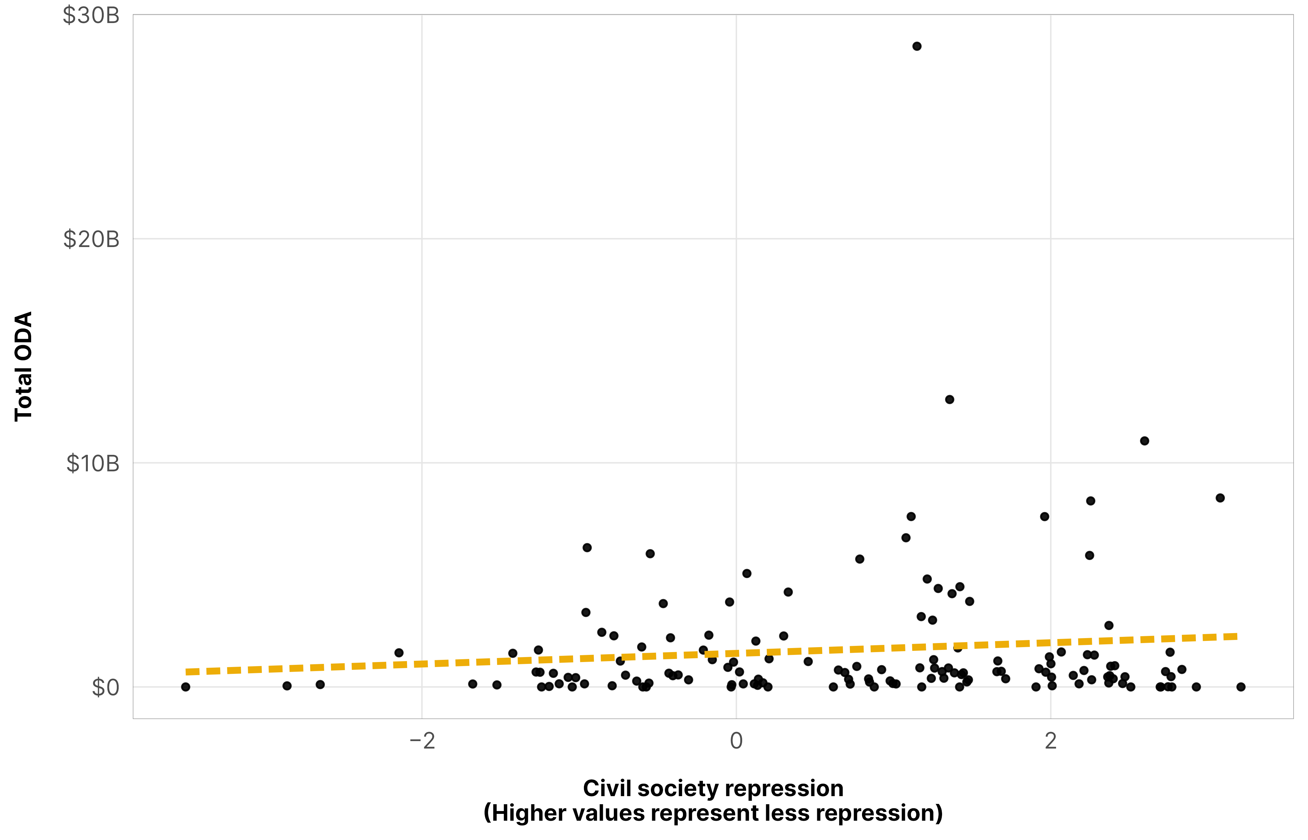
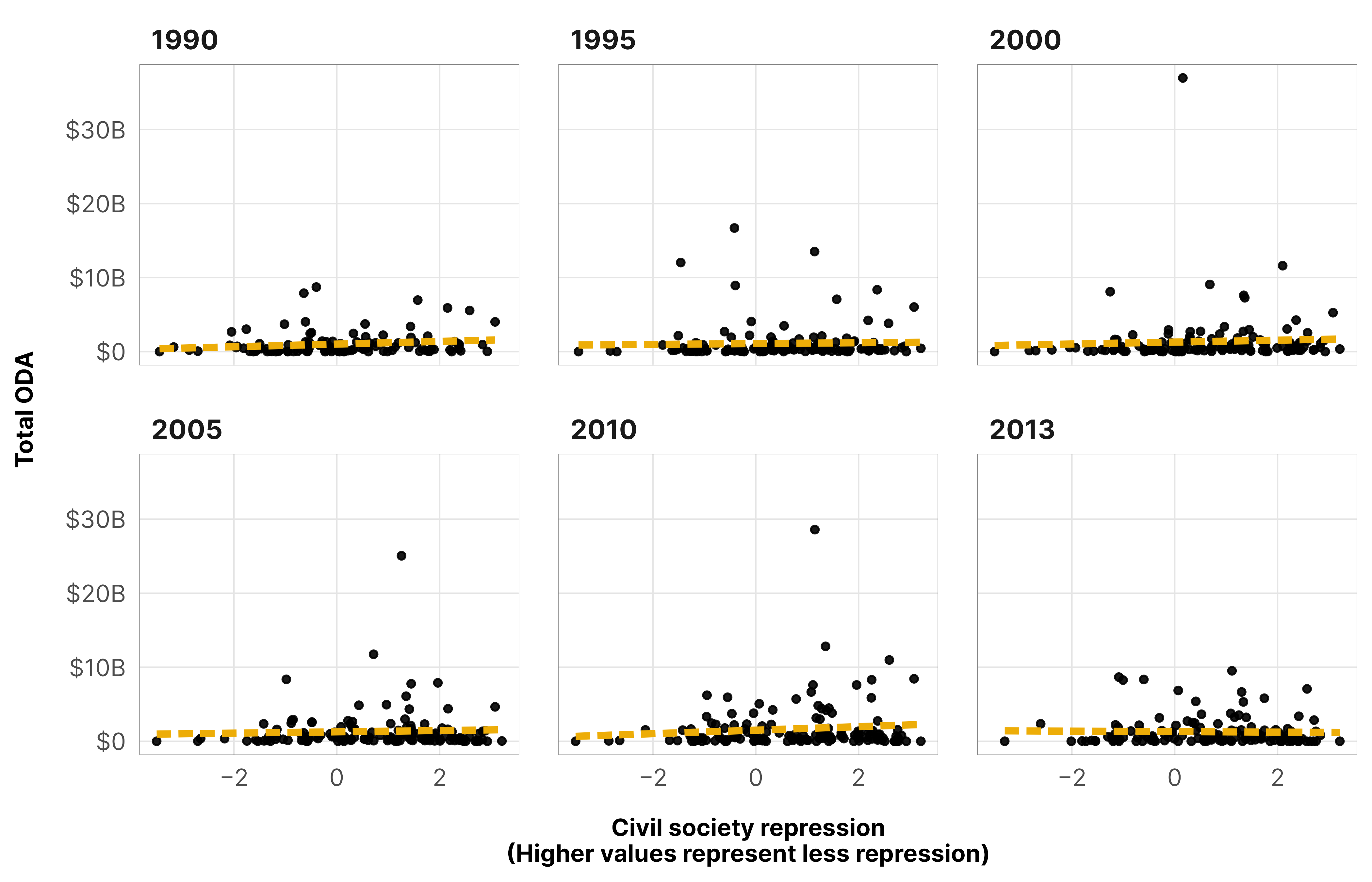
--- title: "Why hierarchical models?" --- ```{r setup, include=FALSE} # tikz stuff # Necessary for using dvisvgm on macOS # See https://www.andrewheiss.com/blog/2021/08/27/tikz-knitr-html-svg-fun/ Sys.setenv (LIBGS = "/usr/local/share/ghostscript/9.53.3/lib/libgs.dylib.9.53" )``` ```{r libraries-data, warning=FALSE, message=FALSE} library (tidyverse)library (targets)library (scales)library (patchwork)tar_config_set (store = here:: here ('_targets' ),script = here:: here ('_targets.R' ))<- list (extra.preamble = c (" \\ usepackage{libertine}" , " \\ usepackage{libertinust1math}" ),dvisvgm.opts = "--font-format=woff" )# Load data # Plotting functions invisible (list2env (tar_read (graphic_functions), .GlobalEnv))invisible (list2env (tar_read (misc_funs), .GlobalEnv))<- tar_read (country_aid_final)<- filter (df_country_aid, laws)``` # Hierarchical structure ```{r data-summary, include=FALSE} <- df_country_aid_laws %>% distinct (year) %>% summarize (num_years = n (),year_first = min (year),year_last = max (year)) %>% bind_cols (tibble (num_countries = df_country_aid_laws %>% distinct (gwcode) %>% nrow ())) %>% as.list ()``` `r details$num_countries` countries across `r details$num_years` years (from `r details$year_first` –`r details$year_last` ). This kind of time series cross-sectional (TSCS) data reflects a natural hierarchical structure, with repeated yearly observations nested within countries ([ see this whole guide I wrote ](https://www.andrewheiss.com/blog/2021/12/01/multilevel-models-panel-data-guide/) because of this exact project)```{tikz panel-structure-svg, engine.opts=font_opts} #| echo: false #| fig-cap: "Multilevel panel data structure, with yearly observations of $y$ nested in countries" #| fig-align: center #| fig-ext: svg #| out-width: 100% \usetikzlibrary{positioning} \usetikzlibrary{shapes.geometric} \definecolor{red}{HTML}{CC503E} \definecolor{teal1}{HTML}{2a5674} \definecolor{teal2}{HTML}{68abb8} \definecolor{teal3}{HTML}{85c4c9} \definecolor{teal4}{HTML}{a8dbd9} \definecolor{peach1}{HTML}{f59e72} \definecolor{peach2}{HTML}{f8b58b} \definecolor{peach3}{HTML}{facba6} \begin{tikzpicture}[{every node/.append style}=draw] \node [rectangle,fill=teal2] (country1) at (0, 2.5) {Country 1}; \node [ellipse,fill=peach1] (y11) at (-1.85, 1) {$y_{i,{t = 1990}_1}$}; \node [ellipse,fill=peach1] (y21) at (0, 1) {$y_{i,{t = t}_1}$}; \node [ellipse,fill=peach1] (y31) at (1.85, 1) {$y_{i,{t = 2013}_1}$}; \draw [-latex] (country1) to (y11); \draw [-latex] (country1) to (y21); \draw [-latex] (country1) to (y31); \node [rectangle,fill=teal3] (country2) at (5.35, 2.5) {Country 2}; \node [ellipse,fill=peach2] (y12) at (4.15, 1) {$y_{i,{1990}_2}$}; \node [draw=none] (y22) at (5.35, 1) {$\dots$}; \node [ellipse,fill=peach2] (y32) at (6.55, 1) {$y_{i,{2013}_2}$}; \draw [-latex] (country2) to (y12); \draw [-latex] (country2) to (y22); \draw [-latex] (country2) to (y32); \node [draw=none] (dots_top) at (7.85, 2.5) {$\dots$}; \node [draw=none] (dots_bottom) at (7.85, 1) {$\dots$}; \draw [-latex] (dots_top) to (dots_bottom); \node [rectangle,fill=teal4] (country_142) at (10.6, 2.5) {Country 142}; \node [ellipse,fill=peach3] (y1_142) at (9.25, 1) {$y_{i,{1990}_{142}}$}; \node [draw=none] (y2_142) at (10.6, 1) {$\dots$}; \node [ellipse,fill=peach3] (y3_142) at (11.95, 1) {$y_{i,{2013}_{142}}$}; \draw [-latex] (country_142) to (y1_142); \draw [-latex] (country_142) to (y2_142); \draw [-latex] (country_142) to (y3_142); \node [rectangle,fill=teal1,text=white] (population) at (5, 4) {Countries eligible for aid}; \draw [-latex] (population) to (country1); \draw [-latex] (population) to (country2); \draw [-latex] (population) to (dots_top); \draw [-latex] (population) to (country_142); \end{tikzpicture} ``` ```{r plot-biggest-movers, warning=FALSE} #| out-width: 80% <- df_country_aid_laws %>% group_by (country) %>% filter (! any (total_oda == 0 )) %>% summarize (across (c (v2csreprss, total_oda), lst (min, max, diff = ~ max (.) - min (.))))<- top_n (biggest_movers, 15 , v2csreprss_diff) %>% filter (country %in% top_n (biggest_movers, 15 , total_oda_diff)$ country) %>% top_n (3 , v2csreprss_diff)<- df_country_aid_laws %>% mutate (highlight_country = ifelse (country %in% top_overall$ country, "Other" ),highlight_country = factor (highlight_country, ordered = TRUE ),highlight_country = fct_relevel (highlight_country, "Other" , after = Inf )) %>% mutate (highlight = highlight_country != "Other" )ggplot (df_cs_oda_highlight, aes (x = v2csreprss, y = total_oda, group = country)) + geom_point (size = 0.15 , alpha = 0.10 ) + geom_smooth (method = "lm" , aes (group = NULL ), color = clrs$ Prism[6 ], linewidth = 1.25 , linetype = "21" , se = FALSE , formula = y ~ x) + geom_path (aes (color = highlight_country, size = highlight),arrow = arrow (type = "open" , angle = 30 , length = unit (0.75 , "lines" )),key_glyph = "timeseries" ) + scale_y_continuous (trans = "log1p" , breaks = c (1e7 , 1e8 , 1e9 , 1e10 , 1e11 ),labels = label_dollar (scale_cut = cut_short_scale ())) + scale_size_manual (values = c (0.045 , 1.25 ), guide = "none" ) + scale_color_manual (values = c (clrs$ Prism[2 ], clrs$ Prism[7 ], clrs$ Prism[9 ], "grey50" ),guide = guide_legend (override.aes = list (linewidth = 1 ))) + coord_cartesian (ylim = c (1e7 , 1e11 )) + labs (x = "Civil society repression \n (Higher values represent less repression)" ,y = "Total ODA" , color = NULL , size = NULL ) + theme_donors ()``` ```{r plot-repression-aid-2010} #| out-width: 80% <- df_country_aid_laws %>% filter (year == 2010 )ggplot (df_country_aid_2010, aes (x = v2csreprss, y = total_oda)) + geom_point (size = 1 , alpha = 0.9 ) + geom_smooth (method = "lm" , color = clrs$ Prism[6 ], linewidth = 1.25 , linetype = "21" , se = FALSE , formula = y ~ x) + scale_x_continuous (labels = label_number (style_negative = "minus" )) + scale_y_continuous (labels = label_dollar (scale_cut = cut_short_scale ())) + labs (x = "Civil society repression \n (Higher values represent less repression)" ,y = "Total ODA" ) + theme_donors ()``` ```{r plot-repression-aid-a-few} #| out-width: 80% <- df_country_aid_laws %>% filter (year %in% c (1990 , 1995 , 2000 , 2005 , 2010 , 2013 ))ggplot (df_country_aid_a_few, aes (x = v2csreprss, y = total_oda)) + geom_point (size = 1 , alpha = 0.9 ) + geom_smooth (method = "lm" , color = clrs$ Prism[6 ], linewidth = 1.25 , linetype = "21" , se = FALSE , formula = y ~ x) + scale_x_continuous (labels = label_number (style_negative = "minus" )) + scale_y_continuous (labels = label_dollar (scale_cut = cut_short_scale ())) + labs (x = "Civil society repression \n (Higher values represent less repression)" ,y = "Total ODA" ) + facet_wrap (vars (year)) + theme_donors ()```