Working with tricky outcomes with lots of zeros

Code

library(tidyverse)
library(targets)
library(brms)
library(tidybayes)
library(scales)
library(patchwork)
library(ggtext)
library(ggh4x)
library(kableExtra)
library(broom.mixed)
library(marginaleffects)
library(extraDistr)

tar_config_set(store = here::here('_targets'),
               script = here::here('_targets.R'))

set.seed(1234)

# Load stuff from targets
# Plotting functions
invisible(list2env(tar_read(graphic_functions), .GlobalEnv))

tar_load(c(m_oda_prelim_time_only_total, m_purpose_prelim_time_only_total))

df_country_aid <- tar_read(country_aid_final)
df_country_aid_laws <- filter(df_country_aid, laws)
df_country_aid_usaid <- df_country_aid_laws %>% 
  filter(year > 2000 & year < 2013)

# Tell bayesplot to use the sunset palette for things like pp_check()
bayesplot::color_scheme_set(clrs$Sunset[2:7])

Complex models

Throughout this project, we use more complex Bayesian models (multilevel hurdle models and zero-inflated models) instead of basic OLS because the data we’re working with is more complex. The complexity in the data leads to complexity in the models, which leads to complexity in the code. Keeping track of and working with all the different moving parts of these models is tricky. As Richard McElreath says,

[A]s models become more monstrous, so too does the code needed to compute predictions and display them. With power comes hardship. It’s better to see the guts of the machine than to live in awe or fear of it. (McElreath 2020, 391)

This document is a basic guide showcasing the entire complexity of the hurdle and zero-inflated models, walking through their formal specifications, how specify priors, how to fit the models and extract posteriors, and how to analyze the posteriors at a population-level and group-level for all the different portions (i.e. non-zero vs. zero) of these models. This document is not our actual analysis—for the sake of simplicity, we only illustrate the effect of year on our outcomes, like outcome ~ year + (1 + year | country). Instead, this document is an illustration and reference for ourselves.

The problem with zeros

All of our outcome variables have a substantial and nontrivial number of zeros in them:

Code

bind_rows(
  `Total ODA (H1)` = count(df_country_aid_laws, is_zero = total_oda == 0),
  `Proportion of contentious aid (H2)` = count(df_country_aid_laws, is_zero = prop_contentious == 0),
  `Proportion of aid to domestic NGOs (H3)` = count(df_country_aid_usaid, is_zero = prop_ngo_dom == 0),
  `Proportion of aid to foreign NGOs (H3)` = count(df_country_aid_usaid, is_zero = prop_ngo_foreign == 0),
  .id = "Outcome"
) %>% 
  group_by(Outcome) %>% 
  mutate(`Number of 0s` = glue::glue("{n[2]} / {sum(n)}")) %>% 
  mutate(`Proportion of 0s` = label_percent(accuracy = 0.1)(n / sum(n))) %>% 
  ungroup() %>% 
  filter(is_zero) %>% select(-is_zero, -n) %>% 
  kbl(align = c("l", "c", "c")) %>% 
  kable_styling(htmltable_class = "table table-sm",
                full_width = FALSE)

Table 1: 0s in our main outcome variables
Outcome	Number of 0s	Proportion of 0s
Total ODA (H1)	198 / 3293	6.0%
Proportion of contentious aid (H2)	479 / 3293	14.5%
Proportion of aid to domestic NGOs (H3)	468 / 1676	27.9%
Proportion of aid to foreign NGOs (H3)	390 / 1676	23.3%

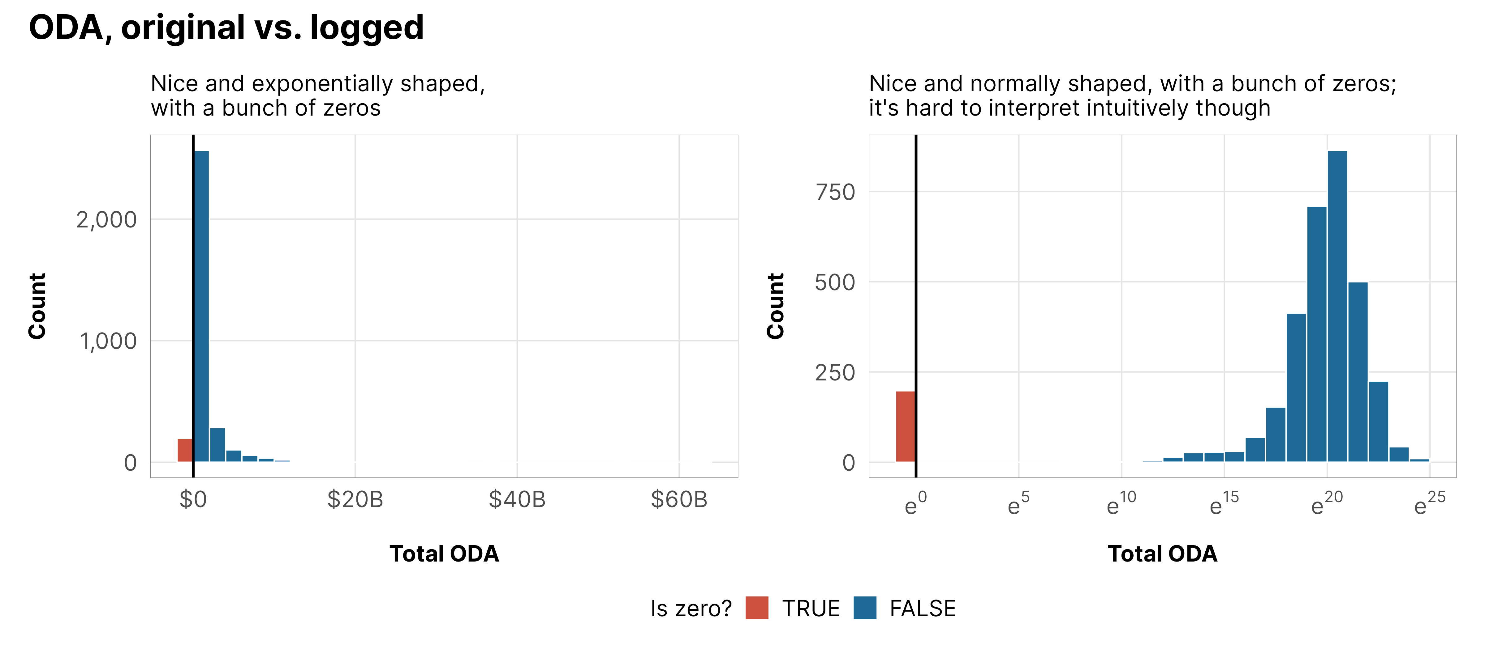
Here’s what that looks like with foreign aid:

Code

plot_dist_unlogged <- df_country_aid_laws %>%
  mutate(is_zero = total_oda == 0) %>% 
  mutate(total_oda = ifelse(is_zero, -0.1, total_oda))  %>%  
  ggplot(aes(x = total_oda)) +
  geom_histogram(aes(fill = is_zero), binwidth = 2e9, 
                 linewidth = 0.25, boundary = 0, color = "white") +
  geom_vline(xintercept = 0) + 
  scale_x_continuous(labels = label_dollar(scale_cut = cut_short_scale())) +
  scale_y_continuous(labels = label_comma()) +
  scale_fill_manual(values = c(clrs$Prism[2], clrs$Prism[8]), 
                    guide = guide_legend(reverse = TRUE)) +
  labs(x = "Total ODA", y = "Count", fill = "Is zero?",
       subtitle = "Nice and exponentially shaped,\nwith a bunch of zeros") +
  theme_donors() +
  theme(legend.position = "bottom")

plot_dist_logged <- df_country_aid_laws %>%
  mutate(is_zero = total_oda_log == 0) %>% 
  mutate(total_oda_log = ifelse(is_zero, -0.1, total_oda_log))  %>%  
  ggplot(aes(x = total_oda_log)) +
  geom_histogram(aes(fill = is_zero), binwidth = 1, 
                 linewidth = 0.25, boundary = 0, color = "white") +
  geom_vline(xintercept = 0) +
  scale_x_continuous(labels = label_math(e^.x)) +
  scale_fill_manual(values = c(clrs$Prism[2], clrs$Prism[8]), 
                    guide = guide_legend(reverse = TRUE)) +
  labs(x = "Total ODA", y = "Count", fill = "Is zero?",
       subtitle = "Nice and normally shaped, with a bunch of zeros;\nit's hard to interpret intuitively though") +
  theme_donors() +
  theme(legend.position = "bottom")

(plot_dist_unlogged | plot_dist_logged) +
  plot_layout(guides = "collect") +
  plot_annotation(title = "ODA, original vs. logged",
                  theme = theme(plot.title = element_text(family = "Inter", face = "bold"),
                                legend.position = "bottom"))

And with the proportion variables:

Code

p1 <- df_country_aid_laws %>%
  mutate(is_zero = prop_contentious == 0) %>% 
  mutate(prop_contentious = ifelse(is_zero, -0.05, prop_contentious))  %>%  
  ggplot(aes(x = prop_contentious)) +
  geom_histogram(aes(fill = is_zero), binwidth = 0.05, 
                 linewidth = 0.25, boundary = 0, color = "white") +
  geom_vline(xintercept = 0) + 
  scale_x_continuous(labels = label_percent()) +
  scale_y_continuous(labels = label_comma()) +
  scale_fill_manual(values = c(clrs$Prism[2], clrs$Prism[8]), 
                    guide = guide_legend(reverse = TRUE)) +
  labs(x = "Proportion of contentious aid", y = "Count", fill = "Is zero?") +
  coord_cartesian(ylim = c(0, 1500)) +
  theme_donors() +
  theme(legend.position = "bottom")

p2 <- df_country_aid_usaid %>%
  mutate(is_zero = prop_ngo_dom == 0) %>% 
  mutate(prop_ngo_dom = ifelse(is_zero, -0.05, prop_ngo_dom))  %>%  
  ggplot(aes(x = prop_ngo_dom)) +
  geom_histogram(aes(fill = is_zero), binwidth = 0.05, 
                 linewidth = 0.25, boundary = 0, color = "white") +
  geom_vline(xintercept = 0) + 
  scale_x_continuous(labels = label_percent()) +
  scale_y_continuous(labels = label_comma()) +
  scale_fill_manual(values = c(clrs$Prism[2], clrs$Prism[8]), 
                    guide = guide_legend(reverse = TRUE)) +
  labs(x = "Proportion of aid to domestic NGOs", y = NULL, fill = "Is zero?") +
  coord_cartesian(ylim = c(0, 1500)) +
  theme_donors() +
  theme(legend.position = "bottom")

p3 <- df_country_aid_usaid %>%
  mutate(is_zero = prop_ngo_foreign == 0) %>% 
  mutate(prop_ngo_foreign = ifelse(is_zero, -0.05, prop_ngo_foreign))  %>%  
  ggplot(aes(x = prop_ngo_foreign)) +
  geom_histogram(aes(fill = is_zero), binwidth = 0.05, 
                 linewidth = 0.25, boundary = 0, color = "white") +
  geom_vline(xintercept = 0) + 
  scale_x_continuous(labels = label_percent()) +
  scale_y_continuous(labels = label_comma()) +
  scale_fill_manual(values = c(clrs$Prism[2], clrs$Prism[8]), 
                    guide = guide_legend(reverse = TRUE)) +
  labs(x = "Proportion of aid to foreign NGOs", y = NULL, fill = "Is zero?") +
  coord_cartesian(ylim = c(0, 1500)) +
  theme_donors() +
  theme(legend.position = "bottom")

(p1 | p2 | p3) +
  plot_layout(guides = "collect") +
  plot_annotation(title = "Proportion-based outcomes",
                  theme = theme(plot.title = element_text(family = "Inter", face = "bold"),
                                legend.position = "bottom"))

Hurdle vs. zero-inflated models

These zeros pose a whole host of tricky methodological issues. We could be like economists and just throw OLS at all these, or do what we’ve done in past versions of this paper and just use OLS on logged aid and fractional logit stuff for the proportions, but we can do better—we can model the zeros directly!

In the course of working on this paper, I’ve written a couple complete guides (for future-me, who is now present-me!) about two different approaches for doing this:

Guide for hurdle models (for total ODA)
Guide for zero-inflated models (for proportions)

There’s actually a subtle difference between hurdle models and zero-inflated models, and this Stack Exchange answer explains the distinction exceptionally well.

Put simply, in hurdle models there’s only one way to get a zero in the outcome; in zero-inflated models there are two ways to get a zero in the outcome. Both models use a two-step process:

In the first stage for both types of models, we model if an outcome is either zero or not zero, or if the non-zero data generating process is on or off. It has a probability $\pi$ of being off (or 0) and a probability $1 - \pi$ of being on (or 1)
In the second stage, the two models diverge a little
1. For hurdle models, there is only one way to get a zero, which is handled with the $\pi$ part in the first stage. Predicted values of $y$ in this second stage cannot be zero, so the distribution of $y$ is truncated at $y > 0$. This is done with some fancy math that incorporates the probability of being not zero ($1 - \pi$) and the regular distribution family (Poisson, lognormal, whatever):
  
  \[ \begin{aligned} & \textbf{Hurdle log-normal observation model} \\ y &\sim \operatorname{Hurdle\,log-normal}(\mu, \sigma, \pi) \quad \text{or alternatively,}\\ y &\sim \begin{cases} 0 & \text{with probability } \pi \\ \operatorname{Log-normal}(\mu, \sigma) & \text{with probability } 1 - \pi \end{cases} \\[4pt] \operatorname{logit}(\pi) &= \gamma_0 + \gamma_1 x_1 \\ \log(\mu) &= \beta_0 + \beta_1 x_1 \\ \sigma &\sim \operatorname{Exponential}(1) \\[10pt] & \textbf{Likelihood of zero} \\ \Pr(0 \mid \pi) &= \underbracket[0.25pt]{\Pr(\text{No $y$} \mid \pi)}_{\substack{\text{Probability}\\ \text{of no $y$}}}\ =\ \pi \\[10pt] & \textbf{Hurdle log-normal likelihood} \\ \Pr(y \mid \pi, \mu, \sigma) &= \begin{dcases} \pi & \text{if } y = 0 \\[4pt] \underbracket[0.25pt]{\frac{(1 - \pi) \times \operatorname{Log-normal}(y \mid \mu, \sigma)} {1 - \operatorname{Log-normal}(0 \mid \mu, \sigma)}}_{\text{Will only predict $y > 0$}} & \text{if } y > 0 \end{dcases} \end{aligned} \]
2. For zero-inflated models, there are two ways to get a zero. For example, in section 12.2 in Statistical Rethinking, McElreath (2020) gives an example of monks who can either (1) drink and do no work, or (2) work and transcribe some number of manuscripts. There’s a two-stage process for getting possible 0s here. A monk could transcribe 0 manuscripts because of the $\pi$ on/off process in the first stage (e.g., they decide to drink and not even attempt to copy any manuscripts). Alternatively, the monk could be “on” in the first stage (e.g., they decide to not drink and to work instead), but then they don’t end up transcribing anything (e.g., the final count is 0 because they were slow, lazy, had a difficult manuscript, or whatever).
  
  So we have to incorporate both avenues for getting a 0 into the likelihood for zero. Predicted values of $y$ in this stage can be zero, so unlike hurdle models, this isn’t truncated or anything. We use some distribution family (Poisson, negative binomial, beta, whatever) at this stage and generate predictions where $y \geq 0$.
  
  SUPER WEIRDLY THOUGH, despite its name, zero-inflated Beta regression is actually kinda sorta a hurdle model and not a zero-inflated model because $\operatorname{Beta}(0 \mid \mu, \phi)$ isn’t normally allowed since the Beta distribution typically only covers $0 < y < 1$ or (0, 1) rather than [0, 1]. That is, according to this definition of hurdling vs. zero-inflating, in zero-inflated models zero is still a possible outcome after moving past the first zero/not zero stage, but the Beta distribution typically doesn’t allow for zeros. ::huge-shrug::
  
  \[ \begin{aligned} & \textbf{Zero-inflated Beta observation model} \\ y &\sim \operatorname{Zero-inflated\, Beta}(\pi, \mu, \phi) \quad \text{or alternatively,}\\ y &\sim \begin{cases} 0 & \text{with probability } \pi + [(1 - \pi) \times \operatorname{Beta}(0 \mid \mu, \phi)] \\ \operatorname{Beta}(\mu, \phi) & \text{with probability } (1 - \pi) \times \operatorname{Beta}(y \mid \mu, \phi) \end{cases} \\[4pt] \operatorname{logit}(\pi) &= \gamma_0 + \gamma_1 x_1 \\ \operatorname{logit}(\mu) &= \beta_0 + \beta_1 x_1 \\ \phi &\sim \operatorname{Exponential}(1) \\[10pt] & \textbf{Likelihood of zero} \\ \Pr(0 \mid \pi, \mu, \phi) &= \underbracket[0.25pt]{\Pr(\text{No $y$} \mid \pi)}_{\substack{\text{Probability of} \\ \text{no $y$ at all}}} \ \overbracket[0.25pt]{+}^{\text{or}}\ \underbracket[0.25pt]{\left[\Pr(\text{Yes $y$} \mid \pi) \times \Pr(0 \mid \mu, \phi)\right]}_{\substack{\text{Probability of yes $y$,} \\ \text{but it happens to be 0}}} \\ &= \pi + [(1 - \pi) \times \operatorname{Beta}(0 \mid \mu, \phi)] \\[10pt] & \textbf{Zero-inflated Beta likelihood} \\ \Pr(y \mid \pi, \mu, \phi) &= \begin{cases} \pi + [(1 - \pi) \times \operatorname{Beta}(0 \mid \mu, \phi)] & \text{if } y = 0 \\[4pt] \underbracket[0.25pt]{(1 - \pi) \times \operatorname{Beta}(y \mid \mu, \phi)}_{\text{Will predict $y \geq 0$}} & \text{if } y > 0 \end{cases} \end{aligned} \]

With all that… whatever. This difference doesn’t super matter for us here. We’ll use both of these kinds of families to model our zero-heavy outcomes.

Hurdle models (total aid)

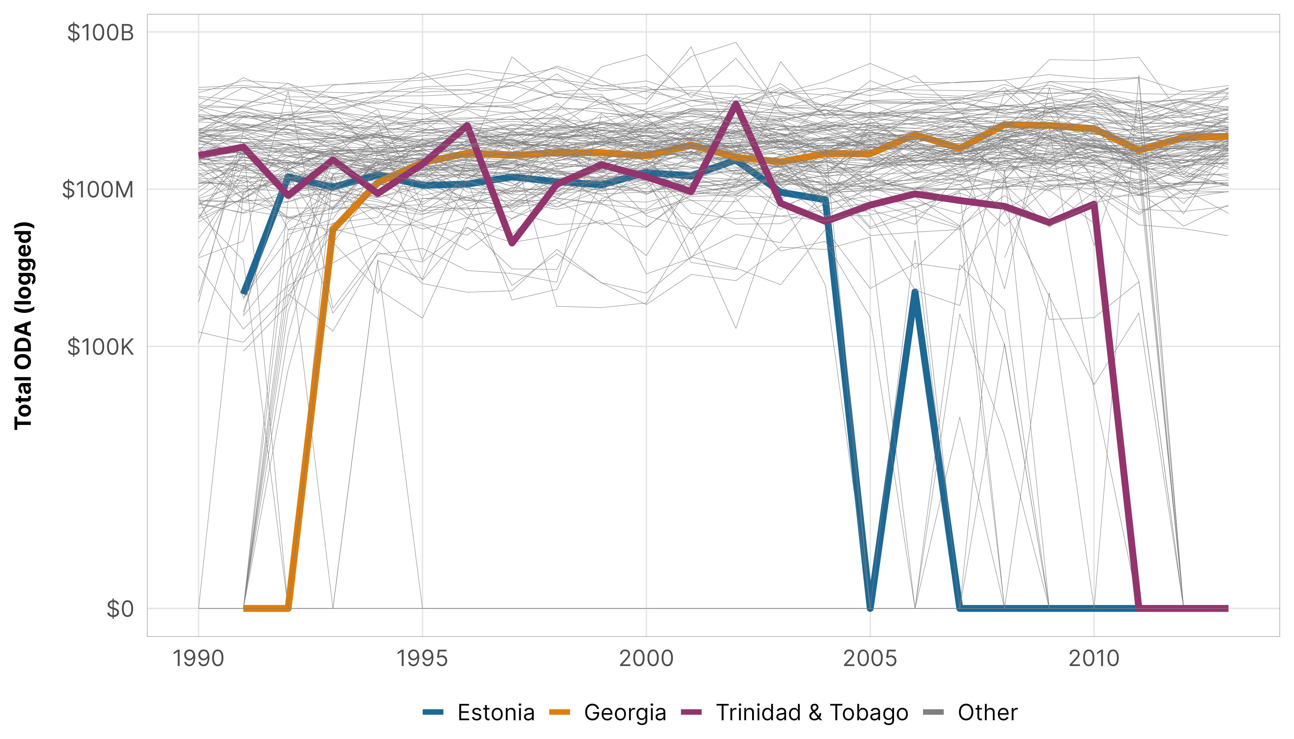
We’re not entirely sure what the actual underlying zero process is for foreign aid, but from looking at the data, we know that there’s a time component—before 1995 and after 2005 lots of countries received no aid. We don’t know why, though. Maybe there are issues with reporting quality. Maybe some countries didn’t need aid anymore (almost like a survival model, but not really, since countries can resume getting aid later after seeing a 0). Maybe there were political reasons. It’s impossible to tell, and it goes beyond the scope of our paper here.

We can see the year-based differences in the presence/absence of 0s in this plot here, with a few countries highlighted to show possible trajectories over time: Georgia starting with 0s then rising to regular levels of aid; Trinidad and Tobago starting with regular levels of aid and then dropping to 0s; Estonia starting with regular levels of aid and then dropping to 0, then resuming aid, then dropping to 0s again.

Code

df_hurdle_highlight <- df_country_aid_laws %>% 
  mutate(highlight_country = ifelse(country %in% c("Estonia", "Georgia", "Trinidad & Tobago"), 
                                    country, "Other"),
         highlight_country = factor(highlight_country, ordered = TRUE),
         highlight_country = fct_relevel(highlight_country, "Other", after = Inf)) %>% 
  mutate(highlight = highlight_country != "Other")

df_hurdle_highlight %>% 
  ggplot(aes(x = year, y = total_oda, group = country, 
             color = highlight_country, linewidth = highlight)) +
  geom_line() +
  scale_y_continuous(trans = "log1p", breaks = c(0, 1e5, 1e8, 1e11),
                     labels = label_dollar(scale_cut = cut_short_scale())) +
  scale_color_manual(values = c(clrs$Prism[2], clrs$Prism[7], clrs$Prism[9], "grey50")) +
  scale_linewidth_discrete(range = c(0.075, 1.25), guide = "none") +
  labs(x = NULL, y = "Total ODA (logged)", color = NULL) +
  guides(color = guide_legend(override.aes = list(linewidth = 1))) +
  theme_donors()

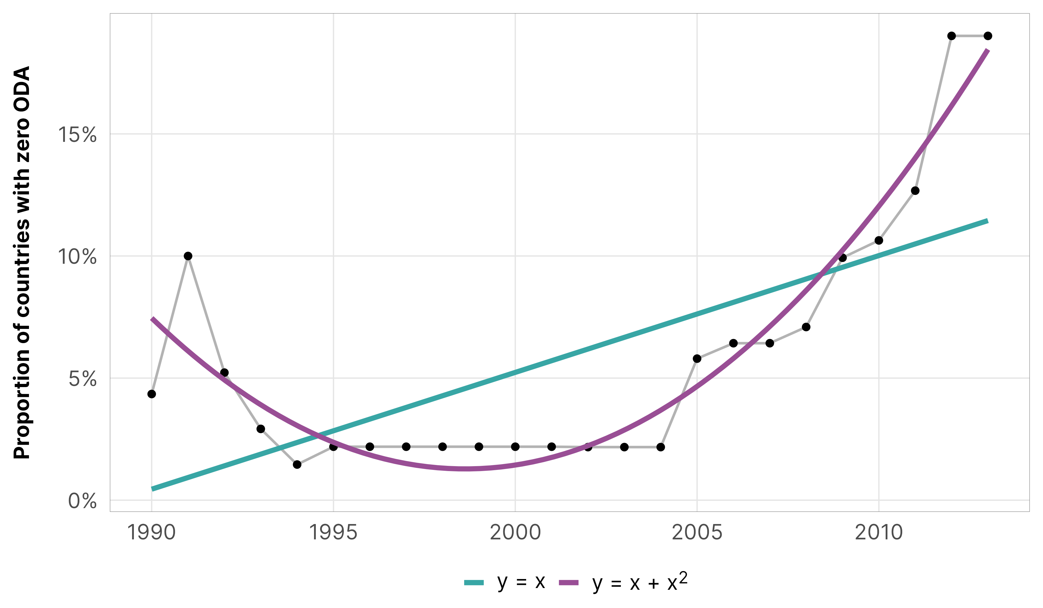
The time trend is even clearer if we plot the proportion of zeros in each year. It actually fits a 2nd-degree polynomial trend really well, but for the sake of simplicity in this example, we’ll just model it as linear and not include a squared term. In our actual models, we use year² in the hurdle part of the model.

Code

df_country_aid_laws %>% 
  group_by(year) %>% 
  summarize(prop_zero = mean(total_oda == 0)) %>% 
  ggplot(aes(x = year, y = prop_zero)) +
  geom_line(linewidth = 0.5, color = "grey70") +
  geom_point(size = 1) + 
  geom_smooth(aes(color = "y = x"), method = "lm", 
              formula = y ~ x, se = FALSE) +
  geom_smooth(aes(color = "y = x + x<sup>2</sup>"), method = "lm", 
              formula = y ~ x + I(x^2), se = FALSE) +
  scale_y_continuous(labels = label_percent()) +
  scale_color_manual(values = clrs$Prism[c(3, 11)]) +
  labs(x = NULL, y = "Proportion of countries with zero ODA",
       color = NULL) +
  theme_donors() +
  theme(legend.text = element_markdown())

Formal statistical model

To account for these dips into 0, we’ll use a hurdle lognormal family (since ODA is exponentially distributed) with a multilevel hierarchical model with country-specific intercepts and a year trend with country-specific offsets (following yet another guide I wrote for this project, this one on multilevel panel data).

We center the year at 2000 so that (1) the intercept is interpretable (Schielzeth 2010) and (2) the MCMC simulation runs faster and more efficiently (McElreath 2020, sec. 13.4, pp. 420–422).

In the actual models we run we include treatment history, independent variables related to civil society, and inverse probability weights, but here since we’re just exploring the mechanics of multilevel hurdle models, we use just a country-and-year-only model.

In {brms}’s random effects syntax, the model formula looks like this:

Code

bf(total_oda ~ year_c + (1 + year_c | gwcode),
   hu ~ year_c)

Equation 1 shows this in more formal mathematical notation, with all the different random effects offsets and priors all working together simultaneously:

\[ \begin{aligned} & \mathrlap{\textbf{Hurdled model of aid $i$ across time $t$ within each country $j$}} \\ \text{Foreign aid}_{it_j} &\sim \mathrlap{\operatorname{Hurdle\,log-normal}(\pi_{it}, \mu_{it_j}, \sigma_y) \quad \text{or alternatively,}} \\ \text{Foreign aid}_{it_j} &\sim \mathrlap{\begin{cases} 0 & \text{with probability } \pi_{it} \\[4pt] \operatorname{Log-normal}(\mu_{it_j}, \sigma_y) & \text{with probability } 1 - \pi_{it} \end{cases}} \\ \\ & \textbf{Models for distribution parameters} \\ \operatorname{logit}(\pi_{it}) &= \gamma_0 + \gamma_1 \text{Year}_{it} & \text{Zero/not-zero process} \\[4pt] \log (\mu_{it_j}) &= (\beta_0 + b_{0_j}) + (\beta_1 + b_{1_j}) \text{Year}_{it_j} & \text{Within-country variation} \\[4pt] \left( \begin{array}{c} b_{0_j} \\ b_{1_j} \end{array} \right) &\sim \text{MV}\,\mathcal{N} \left[ \left( \begin{array}{c} 0 \\ 0 \\ \end{array} \right) , \, \left( \begin{array}{cc} \sigma^2_{0} & \rho_{0, 1}\, \sigma_{0} \sigma_{1} \\ \cdots & \sigma^2_{1} \end{array} \right) \right] & \text{Variability in average intercepts and slopes} \\ \\ & \textbf{Priors} \\ \gamma_0 &\sim \text{Student $t$}(3, -2, 1.5) & \text{Prior for intercept in hurdle model} \\ \gamma_1 &\sim \text{Student $t$}(3, 0, 1.5) & \text{Prior for year effect in hurdle model} \\ \beta_0 &\sim \mathcal{N}(20, 2.5) & \text{Prior for global average aid} \\ \beta_1 &\sim \mathcal{N}(0, 2) & \text{Prior for global year effect} \\ \sigma_y &\sim \operatorname{Exponential}(1) & \text{Prior for within-country variability} \\ \sigma_0 &\sim \operatorname{Exponential}(1) & \text{Prior for between-country intercept variability} \\ \sigma_1 &\sim \operatorname{Exponential}(1) & \text{Prior for between-country slope variability} \\ \rho &\sim \operatorname{LKJ}(2) & \text{Prior for between-country variability} \end{aligned} \tag{1}\]

Prior simulation

For this year-and-country-only model, we set the following priors:

Code

design <- "
  AAABBB
  CCCDDD
  EEFFGG
"

m_oda_prelim_time_only_total$priors %>% 
  parse_dist() %>% 
  # K = dimension of correlation matrix; 
  # ours is 2x2 here because we have one random slope
  marginalize_lkjcorr(K = 2) %>%
  mutate(nice_title = glue::glue("**{class}**: {prior}"),
         stage = ifelse(dpar == "hu", "Hurdle part (π)", "Lognormal part (µ and σ)")) %>% 
  mutate(nice_title = fct_inorder(nice_title)) %>% 
  ggplot(aes(y = 0, dist = .dist, args = .args, fill = prior)) +
  stat_slab(normalize = "panels") +
  scale_fill_manual(values = clrs$Prism[1:6]) +
  facet_manual(vars(stage, nice_title), design = design, scales = "free_x",
               strip = strip_nested(background_x = list(element_rect(fill = "grey92"), NULL),
                                    by_layer_x = TRUE)) +
  guides(fill = "none") +
  labs(x = NULL, y = NULL) +
  theme_donors(prior = TRUE) +
  theme(strip.text = element_markdown())

To make sure these are somewhat reasonable priors, we simulate from them exclusively (following the process outlined in both Statistical Rethinking and Bayes Rules!). Some of these are wild and go into the trillions, but in general they’re in the hundreds-of-millions-of-dollars range, which is good.

These’ll do.

Code

df_country_aid_laws %>%  
  add_epred_draws(m_oda_prelim_time_only_total$model_prior_only, ndraws = 9,
                  seed = 12345) %>% 
  mutate(year = year_c + 2000) %>% 
  ggplot(aes(x = year, y = .epred, group = paste(gwcode, .draw))) +
  geom_line(linewidth = 0.15, color = clrs$Prism[8]) +
  scale_y_log10(labels = label_dollar(scale_cut = cut_short_scale())) +
  coord_cartesian(ylim = c(1e3, 5e11)) +
  facet_wrap(vars(.draw)) +
  labs(x = "Year", y = "Foreign aid", title = "Results sampled from prior only",
       subtitle = "Each panel shows plausible aid-year relationships for 142 simulated countries") +
  theme_donors()

Posterior checks

MCMC diagnostics

Code

m_oda_prelim_time_only_total$model %>% 
  gather_draws(`^b_.*|^sd_.*|^cor_.*|^sigma`, regex = TRUE) %>% 
  ggplot(aes(x = .iteration, y = .value, color = factor(.chain))) +
  geom_line(size = 0.1) +
  scale_color_manual(values = clrs$Sunset[3:6]) +
  facet_wrap(vars(.variable), scales = "free_y") +
  theme_donors()

Code

m_oda_prelim_time_only_total$model %>% 
  gather_draws(`^b_.*|^sd_.*|^cor_.*|^sigma`, regex = TRUE) %>% 
  group_by(.variable) %>% 
  mutate(draw_rank = rank(.value)) %>% 
  ggplot(aes(x = draw_rank, color = factor(.chain))) +
  stat_bin(geom = "step", binwidth = 500, position = position_identity(), boundary = 0) +
  scale_color_manual(values = clrs$Sunset[3:6]) +
  facet_wrap(vars(.variable), scales = "free_y") +
  theme_donors() +
  theme(axis.text.y = element_blank(), axis.title.y = element_blank(), axis.ticks.y = element_blank())

Code

rstan::get_elapsed_time(m_oda_prelim_time_only_total$model$fit)
##         warmup sample
## chain:1   31.0   72.8
## chain:2   29.9   78.3
## chain:3   28.9   65.8
## chain:4   30.7   76.0

rstan::get_elapsed_time(m_oda_prelim_time_only_total$model$fit) %>% 
  as.data.frame() %>% 
  summarize(longest = lubridate::as.duration(max(warmup + sample)))
##                  longest
## 1 108.19s (~1.8 minutes)

Posterior predictive check

Look at that—it all fits so nicely!

Code

withr::with_seed(1234, {
  pp_check(m_oda_prelim_time_only_total$model, ndraws = 20) +
    coord_cartesian(xlim = c(0, 1e10)) +
    labs(x = "Total ODA", title = "Hurdle lognormal model posterior predictive check") +
    scale_x_continuous(labels = label_dollar(scale_cut = cut_short_scale())) +
    theme_donors() +
    theme(axis.text.y = element_blank())
})

Analyzing the posterior

In the actual paper we only interpret the treatment coefficient (total count of barriers, specific barriers, and V-Dem’s civil society index), since that’s all we can legally interpret when doing causal inference—we’ve only identified and closed off one pathway in the DAG, so all the other coefficients are incomplete (Westreich and Greenland 2013; Keele, Stevenson, and Elwert 2020).

Though we only really care about one effect here, we actually have a ton of different parameters to work with—300!

Show the full list of 300 things

get_variables(m_oda_prelim_time_only_total$model)
##   [1] "b_Intercept"                   "b_hu_Intercept"                "b_hu_year_c"                  
##   [4] "b_year_c"                      "sd_gwcode__Intercept"          "sd_gwcode__year_c"            
##   [7] "cor_gwcode__Intercept__year_c" "sigma"                         "r_gwcode[40,Intercept]"       
##  [10] "r_gwcode[41,Intercept]"        "r_gwcode[42,Intercept]"        "r_gwcode[51,Intercept]"       
##  [13] "r_gwcode[52,Intercept]"        "r_gwcode[70,Intercept]"        "r_gwcode[90,Intercept]"       
##  [16] "r_gwcode[91,Intercept]"        "r_gwcode[92,Intercept]"        "r_gwcode[93,Intercept]"       
##  [19] "r_gwcode[94,Intercept]"        "r_gwcode[95,Intercept]"        "r_gwcode[100,Intercept]"      
##  [22] "r_gwcode[101,Intercept]"       "r_gwcode[110,Intercept]"       "r_gwcode[130,Intercept]"      
##  [25] "r_gwcode[135,Intercept]"       "r_gwcode[140,Intercept]"       "r_gwcode[145,Intercept]"      
##  [28] "r_gwcode[150,Intercept]"       "r_gwcode[155,Intercept]"       "r_gwcode[160,Intercept]"      
##  [31] "r_gwcode[165,Intercept]"       "r_gwcode[235,Intercept]"       "r_gwcode[290,Intercept]"      
##  [34] "r_gwcode[310,Intercept]"       "r_gwcode[316,Intercept]"       "r_gwcode[317,Intercept]"      
##  [37] "r_gwcode[339,Intercept]"       "r_gwcode[341,Intercept]"       "r_gwcode[343,Intercept]"      
##  [40] "r_gwcode[344,Intercept]"       "r_gwcode[345,Intercept]"       "r_gwcode[346,Intercept]"      
##  [43] "r_gwcode[347,Intercept]"       "r_gwcode[349,Intercept]"       "r_gwcode[352,Intercept]"      
##  [46] "r_gwcode[355,Intercept]"       "r_gwcode[359,Intercept]"       "r_gwcode[360,Intercept]"      
##  [49] "r_gwcode[365,Intercept]"       "r_gwcode[366,Intercept]"       "r_gwcode[367,Intercept]"      
##  [52] "r_gwcode[368,Intercept]"       "r_gwcode[369,Intercept]"       "r_gwcode[370,Intercept]"      
##  [55] "r_gwcode[371,Intercept]"       "r_gwcode[372,Intercept]"       "r_gwcode[373,Intercept]"      
##  [58] "r_gwcode[404,Intercept]"       "r_gwcode[411,Intercept]"       "r_gwcode[420,Intercept]"      
##  [61] "r_gwcode[432,Intercept]"       "r_gwcode[433,Intercept]"       "r_gwcode[434,Intercept]"      
##  [64] "r_gwcode[435,Intercept]"       "r_gwcode[436,Intercept]"       "r_gwcode[437,Intercept]"      
##  [67] "r_gwcode[438,Intercept]"       "r_gwcode[439,Intercept]"       "r_gwcode[450,Intercept]"      
##  [70] "r_gwcode[451,Intercept]"       "r_gwcode[452,Intercept]"       "r_gwcode[461,Intercept]"      
##  [73] "r_gwcode[471,Intercept]"       "r_gwcode[475,Intercept]"       "r_gwcode[481,Intercept]"      
##  [76] "r_gwcode[482,Intercept]"       "r_gwcode[484,Intercept]"       "r_gwcode[490,Intercept]"      
##  [79] "r_gwcode[500,Intercept]"       "r_gwcode[501,Intercept]"       "r_gwcode[510,Intercept]"      
##  [82] "r_gwcode[516,Intercept]"       "r_gwcode[517,Intercept]"       "r_gwcode[520,Intercept]"      
##  [85] "r_gwcode[522,Intercept]"       "r_gwcode[530,Intercept]"       "r_gwcode[531,Intercept]"      
##  [88] "r_gwcode[540,Intercept]"       "r_gwcode[541,Intercept]"       "r_gwcode[551,Intercept]"      
##  [91] "r_gwcode[552,Intercept]"       "r_gwcode[553,Intercept]"       "r_gwcode[560,Intercept]"      
##  [94] "r_gwcode[565,Intercept]"       "r_gwcode[570,Intercept]"       "r_gwcode[571,Intercept]"      
##  [97] "r_gwcode[572,Intercept]"       "r_gwcode[580,Intercept]"       "r_gwcode[581,Intercept]"      
## [100] "r_gwcode[590,Intercept]"       "r_gwcode[600,Intercept]"       "r_gwcode[615,Intercept]"      
## [103] "r_gwcode[616,Intercept]"       "r_gwcode[620,Intercept]"       "r_gwcode[625,Intercept]"      
## [106] "r_gwcode[626,Intercept]"       "r_gwcode[630,Intercept]"       "r_gwcode[640,Intercept]"      
## [109] "r_gwcode[645,Intercept]"       "r_gwcode[651,Intercept]"       "r_gwcode[652,Intercept]"      
## [112] "r_gwcode[660,Intercept]"       "r_gwcode[663,Intercept]"       "r_gwcode[666,Intercept]"      
## [115] "r_gwcode[670,Intercept]"       "r_gwcode[678,Intercept]"       "r_gwcode[690,Intercept]"      
## [118] "r_gwcode[692,Intercept]"       "r_gwcode[694,Intercept]"       "r_gwcode[696,Intercept]"      
## [121] "r_gwcode[698,Intercept]"       "r_gwcode[700,Intercept]"       "r_gwcode[701,Intercept]"      
## [124] "r_gwcode[702,Intercept]"       "r_gwcode[703,Intercept]"       "r_gwcode[704,Intercept]"      
## [127] "r_gwcode[705,Intercept]"       "r_gwcode[710,Intercept]"       "r_gwcode[712,Intercept]"      
## [130] "r_gwcode[731,Intercept]"       "r_gwcode[732,Intercept]"       "r_gwcode[750,Intercept]"      
## [133] "r_gwcode[760,Intercept]"       "r_gwcode[770,Intercept]"       "r_gwcode[771,Intercept]"      
## [136] "r_gwcode[775,Intercept]"       "r_gwcode[780,Intercept]"       "r_gwcode[790,Intercept]"      
## [139] "r_gwcode[800,Intercept]"       "r_gwcode[811,Intercept]"       "r_gwcode[812,Intercept]"      
## [142] "r_gwcode[816,Intercept]"       "r_gwcode[820,Intercept]"       "r_gwcode[830,Intercept]"      
## [145] "r_gwcode[840,Intercept]"       "r_gwcode[850,Intercept]"       "r_gwcode[860,Intercept]"      
## [148] "r_gwcode[910,Intercept]"       "r_gwcode[940,Intercept]"       "r_gwcode[950,Intercept]"      
## [151] "r_gwcode[40,year_c]"           "r_gwcode[41,year_c]"           "r_gwcode[42,year_c]"          
## [154] "r_gwcode[51,year_c]"           "r_gwcode[52,year_c]"           "r_gwcode[70,year_c]"          
## [157] "r_gwcode[90,year_c]"           "r_gwcode[91,year_c]"           "r_gwcode[92,year_c]"          
## [160] "r_gwcode[93,year_c]"           "r_gwcode[94,year_c]"           "r_gwcode[95,year_c]"          
## [163] "r_gwcode[100,year_c]"          "r_gwcode[101,year_c]"          "r_gwcode[110,year_c]"         
## [166] "r_gwcode[130,year_c]"          "r_gwcode[135,year_c]"          "r_gwcode[140,year_c]"         
## [169] "r_gwcode[145,year_c]"          "r_gwcode[150,year_c]"          "r_gwcode[155,year_c]"         
## [172] "r_gwcode[160,year_c]"          "r_gwcode[165,year_c]"          "r_gwcode[235,year_c]"         
## [175] "r_gwcode[290,year_c]"          "r_gwcode[310,year_c]"          "r_gwcode[316,year_c]"         
## [178] "r_gwcode[317,year_c]"          "r_gwcode[339,year_c]"          "r_gwcode[341,year_c]"         
## [181] "r_gwcode[343,year_c]"          "r_gwcode[344,year_c]"          "r_gwcode[345,year_c]"         
## [184] "r_gwcode[346,year_c]"          "r_gwcode[347,year_c]"          "r_gwcode[349,year_c]"         
## [187] "r_gwcode[352,year_c]"          "r_gwcode[355,year_c]"          "r_gwcode[359,year_c]"         
## [190] "r_gwcode[360,year_c]"          "r_gwcode[365,year_c]"          "r_gwcode[366,year_c]"         
## [193] "r_gwcode[367,year_c]"          "r_gwcode[368,year_c]"          "r_gwcode[369,year_c]"         
## [196] "r_gwcode[370,year_c]"          "r_gwcode[371,year_c]"          "r_gwcode[372,year_c]"         
## [199] "r_gwcode[373,year_c]"          "r_gwcode[404,year_c]"          "r_gwcode[411,year_c]"         
## [202] "r_gwcode[420,year_c]"          "r_gwcode[432,year_c]"          "r_gwcode[433,year_c]"         
## [205] "r_gwcode[434,year_c]"          "r_gwcode[435,year_c]"          "r_gwcode[436,year_c]"         
## [208] "r_gwcode[437,year_c]"          "r_gwcode[438,year_c]"          "r_gwcode[439,year_c]"         
## [211] "r_gwcode[450,year_c]"          "r_gwcode[451,year_c]"          "r_gwcode[452,year_c]"         
## [214] "r_gwcode[461,year_c]"          "r_gwcode[471,year_c]"          "r_gwcode[475,year_c]"         
## [217] "r_gwcode[481,year_c]"          "r_gwcode[482,year_c]"          "r_gwcode[484,year_c]"         
## [220] "r_gwcode[490,year_c]"          "r_gwcode[500,year_c]"          "r_gwcode[501,year_c]"         
## [223] "r_gwcode[510,year_c]"          "r_gwcode[516,year_c]"          "r_gwcode[517,year_c]"         
## [226] "r_gwcode[520,year_c]"          "r_gwcode[522,year_c]"          "r_gwcode[530,year_c]"         
## [229] "r_gwcode[531,year_c]"          "r_gwcode[540,year_c]"          "r_gwcode[541,year_c]"         
## [232] "r_gwcode[551,year_c]"          "r_gwcode[552,year_c]"          "r_gwcode[553,year_c]"         
## [235] "r_gwcode[560,year_c]"          "r_gwcode[565,year_c]"          "r_gwcode[570,year_c]"         
## [238] "r_gwcode[571,year_c]"          "r_gwcode[572,year_c]"          "r_gwcode[580,year_c]"         
## [241] "r_gwcode[581,year_c]"          "r_gwcode[590,year_c]"          "r_gwcode[600,year_c]"         
## [244] "r_gwcode[615,year_c]"          "r_gwcode[616,year_c]"          "r_gwcode[620,year_c]"         
## [247] "r_gwcode[625,year_c]"          "r_gwcode[626,year_c]"          "r_gwcode[630,year_c]"         
## [250] "r_gwcode[640,year_c]"          "r_gwcode[645,year_c]"          "r_gwcode[651,year_c]"         
## [253] "r_gwcode[652,year_c]"          "r_gwcode[660,year_c]"          "r_gwcode[663,year_c]"         
## [256] "r_gwcode[666,year_c]"          "r_gwcode[670,year_c]"          "r_gwcode[678,year_c]"         
## [259] "r_gwcode[690,year_c]"          "r_gwcode[692,year_c]"          "r_gwcode[694,year_c]"         
## [262] "r_gwcode[696,year_c]"          "r_gwcode[698,year_c]"          "r_gwcode[700,year_c]"         
## [265] "r_gwcode[701,year_c]"          "r_gwcode[702,year_c]"          "r_gwcode[703,year_c]"         
## [268] "r_gwcode[704,year_c]"          "r_gwcode[705,year_c]"          "r_gwcode[710,year_c]"         
## [271] "r_gwcode[712,year_c]"          "r_gwcode[731,year_c]"          "r_gwcode[732,year_c]"         
## [274] "r_gwcode[750,year_c]"          "r_gwcode[760,year_c]"          "r_gwcode[770,year_c]"         
## [277] "r_gwcode[771,year_c]"          "r_gwcode[775,year_c]"          "r_gwcode[780,year_c]"         
## [280] "r_gwcode[790,year_c]"          "r_gwcode[800,year_c]"          "r_gwcode[811,year_c]"         
## [283] "r_gwcode[812,year_c]"          "r_gwcode[816,year_c]"          "r_gwcode[820,year_c]"         
## [286] "r_gwcode[830,year_c]"          "r_gwcode[840,year_c]"          "r_gwcode[850,year_c]"         
## [289] "r_gwcode[860,year_c]"          "r_gwcode[910,year_c]"          "r_gwcode[940,year_c]"         
## [292] "r_gwcode[950,year_c]"          "lprior"                        "lp__"                         
## [295] "accept_stat__"                 "treedepth__"                   "stepsize__"                   
## [298] "divergent__"                   "n_leapfrog__"                  "energy__"

142 country-specific intercept offsets: $b_{0_j}$
142 country-specific offsets to the year_c slope: $b_{1_j}$
2 global terms (intercept and year_c) for the $\mu$ part of the model: $\beta_0$ and $\beta_1$
2 global terms (intercept and year_c) for the hurdled $\pi$ part of the model: $\gamma_0$ and $\gamma_1$
The overall within-country $\sigma$: $\sigma_y$
The variability in country-specific intercept and slope offsets: $\sigma^2_0$ and $\sigma^2_1$
The correlation between country-specific slopes and intercepts: $\rho$
8 auxiliary Stan-specific things like lprior, n_leapfrog__, energy__, etc.

Code

m_oda_prelim_time_only_total$model
##  Family: hurdle_lognormal 
##   Links: mu = identity; sigma = identity; hu = logit 
## Formula: total_oda ~ year_c + (1 + year_c | gwcode) 
##          hu ~ year_c
##    Data: dat (Number of observations: 3293) 
##   Draws: 4 chains, each with iter = 5000; warmup = 1000; thin = 1;
##          total post-warmup draws = 16000
## 
## Group-Level Effects: 
## ~gwcode (Number of levels: 142) 
##                       Estimate Est.Error l-95% CI u-95% CI Rhat Bulk_ESS Tail_ESS
## sd(Intercept)             1.51      0.09     1.34     1.70 1.00     1345     3271
## sd(year_c)                0.08      0.01     0.07     0.10 1.00     4844     8660
## cor(Intercept,year_c)    -0.08      0.09    -0.26     0.10 1.00     3632     6793
## 
## Population-Level Effects: 
##              Estimate Est.Error l-95% CI u-95% CI Rhat Bulk_ESS Tail_ESS
## Intercept       19.74      0.13    19.49    20.00 1.00      673     1445
## hu_Intercept    -3.09      0.10    -3.29    -2.91 1.00    24114    12594
## hu_year_c        0.10      0.01     0.07     0.12 1.00    22946    13418
## year_c           0.03      0.01     0.01     0.04 1.00     3278     6130
## 
## Family Specific Parameters: 
##       Estimate Est.Error l-95% CI u-95% CI Rhat Bulk_ESS Tail_ESS
## sigma     1.03      0.01     1.00     1.06 1.00    26366    11425
## 
## Draws were sampled using sample(hmc). For each parameter, Bulk_ESS
## and Tail_ESS are effective sample size measures, and Rhat is the potential
## scale reduction factor on split chains (at convergence, Rhat = 1).

To help with the intuition behind all these coefficients and moving parts in this hurdle model, though, it’s helpful to walk through the different population-level (or global within-country) effects, group level (between-country) effects, and the within- and between-country variability. We also need to walk through these effects at each part of the model—the regular part that models $\mu$ and the hurdled part that models $\pi$.

Non-hurdled vs. hurdled parts (µ vs. π)

Before looking at population/global effects and group/country-level effects, we’ll first explore the different parts of the model. We have three different parts to consider:

\[ \begin{aligned} \text{Foreign aid}_{it_j} &\sim \operatorname{Hurdle\,log-normal}(\pi_{it}, \mu_{it_j}, \sigma_y) & \text{Overall aid} \\ \operatorname{logit}(\pi_{it}) &= \gamma_0 + \gamma_1 \text{Year}_{it} & \text{0/not 0 process} \\ \log (\mu_{it_j}) &= (\beta_0 + b_{0_j}) + (\beta_1 + b_{1_j}) \text{Year}_{it_j} & \text{$\gt 0$ process} \end{aligned} \]

We can explore the posterior distributions for each of these parts using different combinations of the posterior_linpred(), posterior_epred(), and posterior_predict() functions from {brms} (or their {tidybayes} counterparts linpred_draws(), epred_draws(), and predicted_draws()). I have a whole detailed guide about the subtle differences between these (along with cheat sheets!) that I wrote in part because of this paper. See that guide for more details—here I’ll be less verbose and pedagogical.

Zero part (π and γs)

First we can look at the hurdle part ($\operatorname{logit}(\pi_{it})$) that predicts if the outcome is 0 or not 0. In this example, we modeled this just with year, so we have a $\gamma_0$ coefficient for the intercept and a $\gamma_1$ coefficient for the year effect. These are on the logit scale, so exponentiating them will give us an odds ratio and inverse logit-ing them with plogis() will give us probabilities.

Code

# Uninterpretable log odds
m_oda_prelim_time_only_total$model %>% 
  tidy(effects = "fixed") %>% 
  filter(str_starts(term, "hu_"))
## # A tibble: 2 × 7
##   effect component term           estimate std.error conf.low conf.high
##   <chr>  <chr>     <chr>             <dbl>     <dbl>    <dbl>     <dbl>
## 1 fixed  cond      hu_(Intercept)  -3.09      0.0982  -3.29      -2.91 
## 2 fixed  cond      hu_year_c        0.0951    0.0120   0.0720     0.119

# Odds ratios
m_oda_prelim_time_only_total$model %>% 
  tidy(effects = "fixed") %>% 
  filter(str_starts(term, "hu_")) %>% 
  mutate(across(c(estimate, conf.low, conf.high), exp))
## # A tibble: 2 × 7
##   effect component term           estimate std.error conf.low conf.high
##   <chr>  <chr>     <chr>             <dbl>     <dbl>    <dbl>     <dbl>
## 1 fixed  cond      hu_(Intercept)   0.0453    0.0982   0.0371    0.0547
## 2 fixed  cond      hu_year_c        1.10      0.0120   1.07      1.13

The intercept on both the logit and the odds scales is hard to interpret, but we can convert the log odds to the probability with $\frac{e^{\gamma_0}}{1 + e^{\gamma_0}}$ or plogis(), which is 0.043, which means that in the year 2000 (i.e. when year_c is 0), the model predicts that 4.3% of countries received $0 in ODA.

The probability of receiving non-zero ODA increases by $e^{\gamma_1}$ each year after that, or 1.1, or that a one-year increase in time makes it 10% more likely that a country will receive zero aid.

Odds ratios are still weird to work with, so we can use probabilities instead. We can’t just find the inverse logit of $\gamma_1$ due to how logistic regression works—we have to incorporate information from the intercept too:

Code

hurdle_coefs <- m_oda_prelim_time_only_total$model %>% 
  tidy(effects = "fixed")

gamma_0 <- hurdle_coefs %>% filter(term == "hu_(Intercept)") %>% pull(estimate)
gamma_1 <- hurdle_coefs %>% filter(term == "hu_year_c") %>% pull(estimate)

avg_pp_year <- plogis(gamma_0 + gamma_1) - plogis(gamma_0)
avg_pp_year
## b_hu_Intercept 
##        0.00412

This implies that the proportion of zeros increases by 0.004 percentage points per year on average. Because this is a nonlinear model, the exact percentage point increase differs over time. We can instead look at predictions from the model using linpred_draws(dpar = "hu", transform = TRUE). This will calculate predicted values from the $\operatorname{logit}(\pi_{it})$ part of the model. With transform = FALSE, it will return logit-scale values; with transform = TRUE, it will return probability-scale values.

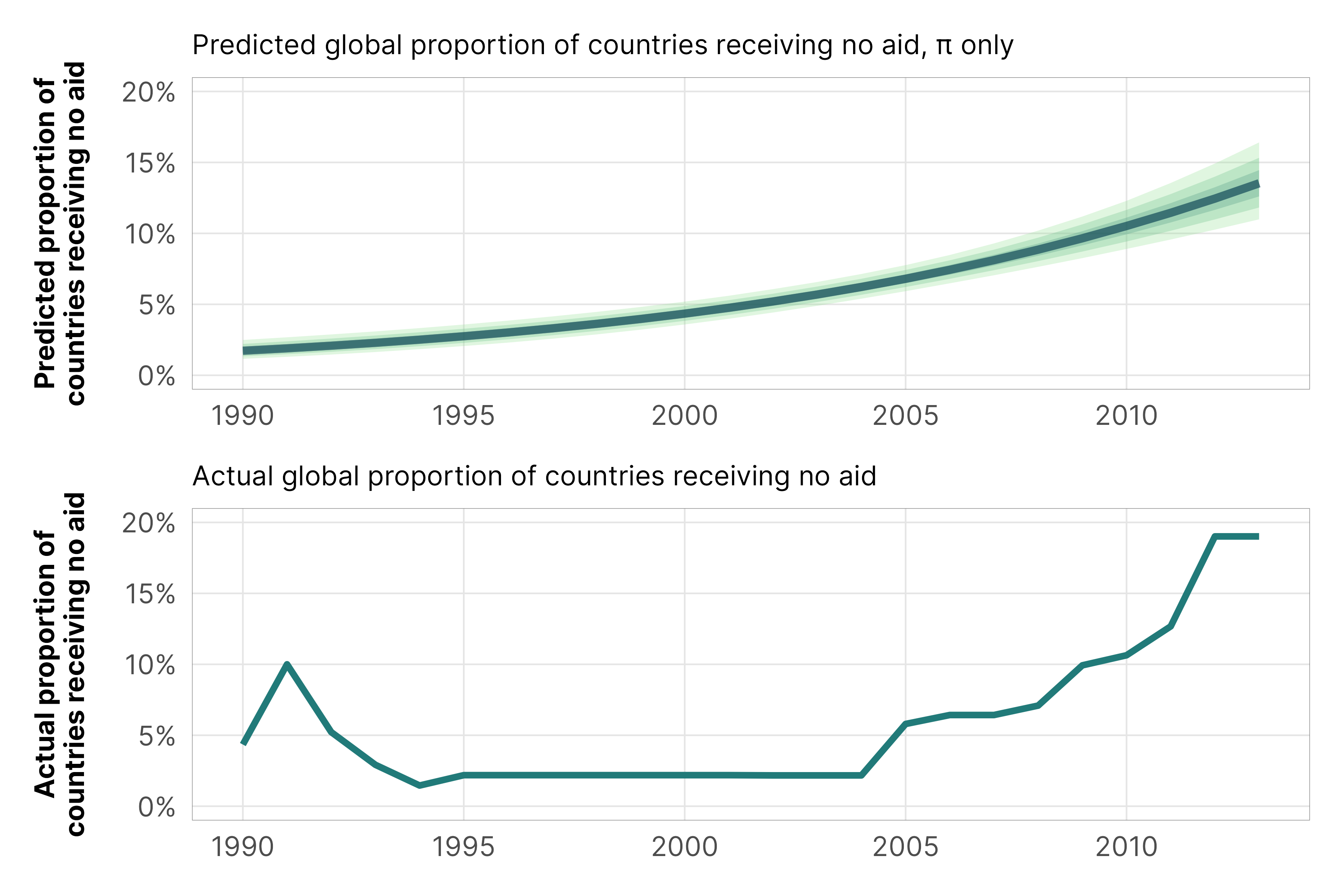
Even if we only account for year in the hurdle part of the model, we do a pretty good job predicting the proportion of zeros over time. In the actual data, there’s an increase in zeros after 2005; in the model predictions we see the same thing (and note that in 2000 the predicted proportion is 4.3%, which is the same as the un-logit-ed intercept coefficient).

Code

plot_hu_hu <- m_oda_prelim_time_only_total$model %>% 
  linpred_draws(newdata = tibble(year_c = seq(-10, 13, 1)),
                re_formula = NA,
                dpar = "hu", transform = TRUE) %>% 
  mutate(year = year_c + 2000) %>% 
  ggplot(aes(x = year, y = hu)) +
  stat_lineribbon(color = clrs$Emrld[7], alpha = 0.3) +
  scale_y_continuous(labels = label_percent()) +
  scale_fill_manual(values = clrs$Emrld[2:4]) +
  guides(fill = "none") +
  labs(x = NULL, y = "Predicted proportion of\ncountries receiving no aid",
       subtitle = "Predicted global proportion of countries receiving no aid, π only") +
  theme_donors()

plot_actual_zeros <- df_country_aid_laws %>% 
  group_by(year) %>% 
  summarize(prop_zero = sum(total_oda == 0) / n()) %>% 
  ggplot(aes(x = year, y = prop_zero)) + 
  geom_line(color = clrs$Emrld[5], linewidth = 1) +
  scale_y_continuous(labels = label_percent()) +
  labs(x = NULL, y = "Actual proportion of\ncountries receiving no aid",
       subtitle = "Actual global proportion of countries receiving no aid") +
  theme_donors()

(plot_hu_hu / plot_actual_zeros) &
  coord_cartesian(ylim = c(0, 0.2))

Non-zero part (µ and βs)

Next we can look at the non-hurdle part ($\log (\mu_{it_j})$) that predicts non-zero outcome values. We modeled this with year, so we have a $\beta_0$ coefficient for the intercept and a $\beta_1$ coefficient for the year slope, but we also have random country-specific offsets for both the intercept and slope. This will complicate life (as explained below!) and means we can’t really interpret these directly. But for now we’ll pretend we can, just to understand how these coefficients work here.

Code

# Logged values
m_oda_prelim_time_only_total$model %>% 
  tidy(effects = "fixed") %>% 
  filter(!str_starts(term, "hu_"))
## # A tibble: 2 × 7
##   effect component term        estimate std.error conf.low conf.high
##   <chr>  <chr>     <chr>          <dbl>     <dbl>    <dbl>     <dbl>
## 1 fixed  cond      (Intercept)  19.7      0.131    19.5      20.0   
## 2 fixed  cond      year_c        0.0266   0.00776   0.0114    0.0417

# Unlogged values
m_oda_prelim_time_only_total$model %>% 
  tidy(effects = "fixed") %>% 
  filter(!str_starts(term, "hu_")) %>% 
  mutate(across(c(estimate, conf.low, conf.high), exp))
## # A tibble: 2 × 7
##   effect component term            estimate std.error     conf.low    conf.high
##   <chr>  <chr>     <chr>              <dbl>     <dbl>        <dbl>        <dbl>
## 1 fixed  cond      (Intercept) 374746463.     0.131   290176524.   482747838.  
## 2 fixed  cond      year_c              1.03   0.00776         1.01         1.04

The intercept here shows that the predicted average level of ODA in 2000 is $e^{19.7}$, or $374,746,463. The year effect on the log scale is hard to think about, but if we exponentiate it like $e^{0.027}$, we get 1.027, which is a multiplier effect like an odds ratio: ODA increases by 2.7% each year.

We can instead look at predictions from the model using linpred_draws(transform = TRUE). This will calculate predicted values from the $\log (\mu_{it_j})$ part of the model. With transform = FALSE, it will return log-scale values; with transform = TRUE, it will return dollar-scale values. We could technically include dpar = "mu" to specify that we want values from the $\mu$ part of the model, but that’s also just the default, so there’s no need.

The predicted value in 2000 is $374,746,463, like we found earlier. The line goes up, as expected. We could use {marginaleffects} to find the exact slope at a variety of locations along that line, but we’ll skip that for now because doing that requires more nuance, given the multilevel nature of the model (more on that below!)

Code

plot_hu_mu_linpred <- m_oda_prelim_time_only_total$model %>% 
  linpred_draws(newdata = tibble(year_c = seq(-10, 13, 1)),
                re_formula = NA, dpar = "mu") %>% 
  mutate(.linpred = exp(.linpred)) %>% 
  mutate(year = year_c + 2000) %>% 
  ggplot(aes(x = year, y = .linpred)) +
  stat_lineribbon(color = clrs$PurpOr[7], alpha = 0.3) +
  scale_y_continuous(labels = label_dollar(scale_cut = cut_short_scale())) +
  scale_fill_manual(values = clrs$PurpOr[3:5]) +
  guides(fill = "none") +
  labs(x = NULL, y = "Predicted foriegn aid",
       subtitle = "Predicted global average foreign aid, µ only") +
  theme_donors()
plot_hu_mu_linpred

Combined processes (y)

Finally, we can look at both the hurdle ($\operatorname{logit}(\pi_{it})$) and non-hurdle ($\log (\mu_{it_j})$) parts of the model simultaneously. Recall from the formal model that the outcome is a function of both the $\pi$ part and the $\mu$ part:

\[ \text{Foreign aid}_{it_j} \sim \operatorname{Hurdle\,log-normal}(\pi_{it}, \mu_{it_j}, \sigma_y) \]

We can work with both of these parts simultaneously if we use epred_draws() instead of linpred_draws(), which calculates the expectation (the “e” in epred) of the posterior predictive distribution of the outcome, or $\textbf{E}(\text{Foreign aid}_{it_j})$.

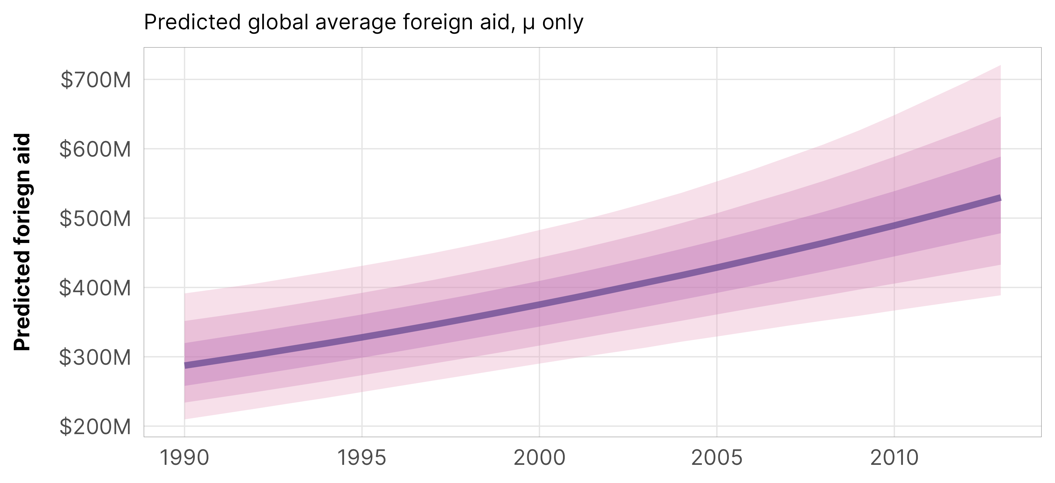
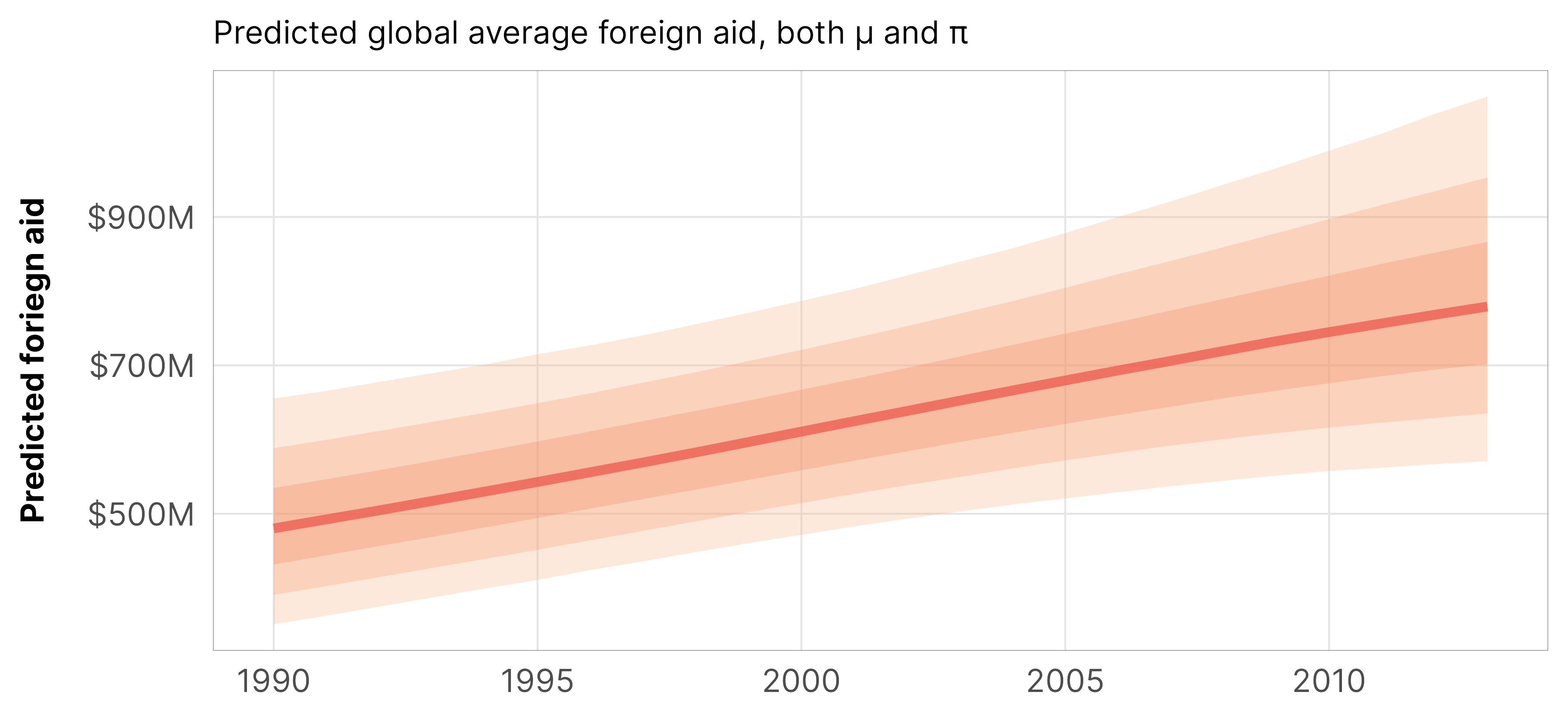
The plot of epred values is different from the linear predictor we found with the $\mu$ part only—that’s because we’re now also incorporating the zero/non-zero process. In general the whole line is shift up higher—instead of ≈$400 million in 2000, we now see ≈$600ish million. The slope of the line is also a little wonky and dampened in later years—this is because the probability of zero aid is higher after 2005.

Code

plot_hu_epred <- m_oda_prelim_time_only_total$model %>% 
  epred_draws(newdata = tibble(year_c = seq(-10, 13, 1)),
              re_formula = NA) %>% 
  mutate(year = year_c + 2000) %>% 
  ggplot(aes(x = year, y = .epred)) +
  stat_lineribbon(color = clrs$Peach[7], alpha = 0.3) +
  scale_y_continuous(labels = label_dollar(scale_cut = cut_short_scale())) +
  scale_fill_manual(values = clrs$Peach[3:5]) +
  guides(fill = "none") +
  labs(x = NULL, y = "Predicted foriegn aid",
       subtitle = "Predicted global average foreign aid, both µ and π") +
  theme_donors()
plot_hu_epred

Here’s what all three of these plots look like simultaneously (just the $\pi$ hurdling part, just the $\mu$ non-hurdled part, and the combined epred part):

Code

(plot_hu_hu / plot_hu_mu_linpred / plot_hu_epred) +
  plot_annotation(title = "Conditional effect of time on foreign aid",
                  subtitle = "total_aid ~ year + (1 + year | country)\nhu ~ year",
                  theme = theme(plot.title = element_text(family = "Inter", face = "bold"),
                                plot.subtitle = element_text(family = "Inconsolata")))

Global analysis (βs)

We looked at the coefficients for the non-hurdle-part intercept and slope up above, but that was a little wrong because of how multilevel models work. To show why (and to show how to actually interpret these things correctly), we’ll look at the relationship between year and aid for the typical country, or just the global $\beta_0$ and the global $\beta_1$. Because we’re using a generalized linear mixed model (GLMM), this is tricky! With normal Gaussian regression, we can interpret the $\beta_0$ and $\beta_1$ coefficients directly (and that’s what Bayes Rules! teaches here, for instance). But GLMMs have link functions, which add a whole extra layer of complexity.

With GLMMs, we can talk about two different kinds of average global effects, or the confusingly named (1) conditional effects and (2) marginal effects. I have a whole blog post guide about the distinction and how to calculate them (I actually wrote that post because of this project). The distinction between the two seems semantic but it’s actually really quite important:

Conditional effect = average country: All $b_n$ offsets are set to 0 so that the effects or coefficients represent the effect in a typical country with the global average level of a variable.
Marginal effect = countries on average: All $b_n$ offsets are dealt with mathematically (averaged/marginalized out or integrated out) so that the effects or coefficients represent the effect of a variable across all countries on average.

In general, we’re more interested in conditional effects, since Muff, Held, and Keller (2016) argue that conditional models (i.e. average/typical country where offsets are set to 0) are the “more powerful choice to explain how covariates are associated with a non-normal response” rather than marginal models (i.e. countries on average). But we explore both here, because why not.

Conditional effects

Since the effect of year here is continuous, we can’t just define the ATE as a contrast between when it is 1 vs. when it is 0. Instead, we want the instantaneous effect, or instantaneous slope/partial derivative of year. Rather than figure out the formal calculus for that, we’ll use marginaleffects() to calculate the numerical derivative, which finds the predicted value of $Y$ at some value of $X$, finds the predicted value of $Y$ at some value of $X$ plus a tiny bit ($\varepsilon$ here), subtracts them, and divides by $\varepsilon$. For our situation here, it looks like this mess:

\[ \frac{\textbf{E}(\text{ODA}_{i_j} \mid \{b_{0_j}, b_{0_j}\} = 0, \text{Year} = t + \varepsilon) - \textbf{E}(\text{ODA}_{i_j} \mid \{b_{0_j}, b_{0_j}\} = 0, \text{Year} = t)}{\varepsilon} \]

{brms}’s syntax for $\{b_{0_j}, b_{0_j}\} = 0$ (i.e. setting all the random offsets to zero) is to use re_formula = NA in the different functions that generate predictions.

To see what this estimand looks like, it’s helpful to first look at range of predicted values of ODA so we can see what line we’re finding the slope for. To help with the intuition we’ll look at the plots on both the link (log) scale and the back-transformed response (dollar) scale.

We can do this automatically with marginaleffects::plot_cap():

Code

# Log scale
plot_cap(m_oda_prelim_time_only_total$model, 
         condition = "year_c", type = "link", 
         re_formula = NA)

# Dollar scale
plot_cap(m_oda_prelim_time_only_total$model, 
         condition = "year_c", type = "response", 
         re_formula = NA)

Or more manually with epred_draws():

Code

preds_log_hu <- m_oda_prelim_time_only_total$model %>% 
  linpred_draws(newdata = tibble(year_c = seq(-10, 13, 1)),
                re_formula = NA) %>% 
  mutate(year = year_c + 2000) %>% 
  ggplot(aes(x = year, y = .linpred)) +
  stat_lineribbon(color = clrs$Peach[7]) +
  scale_y_continuous(labels = label_math(e^.x)) +
  scale_fill_manual(values = clrs$Peach[1:3]) +
  guides(fill = "none") +
  labs(x = NULL, y = "Predicted log foriegn aid") +
  theme_donors()

preds_dollar_hu <- m_oda_prelim_time_only_total$model %>% 
  epred_draws(newdata = tibble(year_c = seq(-10, 13, 1)),
              re_formula = NA) %>% 
  mutate(year = year_c + 2000) %>% 
  ggplot(aes(x = year, y = .epred)) +
  stat_lineribbon(color = clrs$Peach[7]) +
  scale_y_continuous(labels = label_dollar(scale_cut = cut_short_scale())) +
  scale_fill_manual(values = clrs$Peach[1:3]) +
  guides(fill = "none") +
  labs(x = NULL, y = "Predicted foriegn aid") +
  theme_donors()

preds_log_hu | preds_dollar_hu

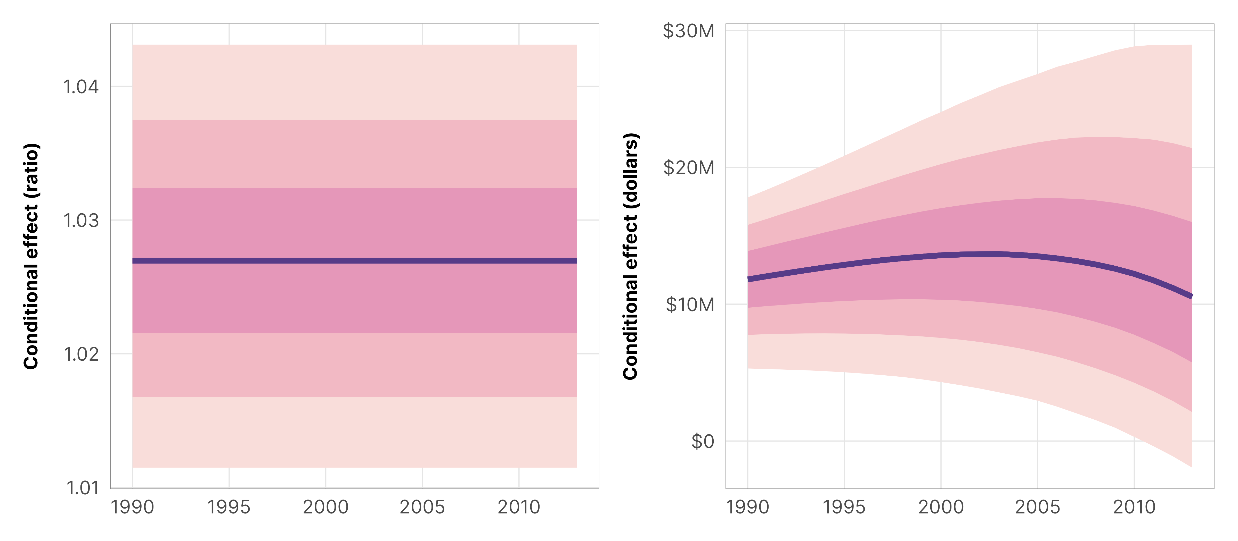
The slopes of both of these lines are actually fairly straight. On the log scale, the slope is constant and linear; on the dollar scale, the slope is generally pretty constant, though it starts to think about leveling out a tiny bit after 2005—that’s because of the increased probability of seeing $0 in ODA starting in that year.

We can use marginaleffects() to get the exact slope of those lines at any value of year_c that we want, and we can plot those slopes across the whole range of years. On the log scale, the line is flat, since the slope is constant; on the dollar scale, it is mostly flat, with a slight drop in later years

Code

mfx_log_hu <- marginaleffects(
  m_oda_prelim_time_only_total$model, 
  newdata = datagrid(year_c = seq(-10, 13, by = 1)),
  variables = "year_c",
  type = "link",
  re_formula = NA
)

mfx_dollar_hu <- marginaleffects(
  m_oda_prelim_time_only_total$model, 
  newdata = datagrid(year_c = seq(-10, 13, by = 1)),
  variables = "year_c",
  type = "response",
  re_formula = NA
)

Code

plot_mfx_log_hu <- mfx_log_hu %>% 
  posteriordraws() %>% 
  mutate(year = year_c + 2000) %>% 
  ggplot(aes(x = year, y = exp(draw))) +
  stat_lineribbon(color = clrs$PurpOr[7]) +
  scale_fill_manual(values = clrs$PurpOr[1:3]) +
  guides(fill = "none") +
  labs(x = NULL, y = "Conditional effect (ratio)") +
  theme_donors()

plot_mfx_dollar_hu <- mfx_dollar_hu %>% 
  posteriordraws() %>% 
  mutate(year = year_c + 2000) %>% 
  ggplot(aes(x = year, y = draw)) +
  stat_lineribbon(color = clrs$PurpOr[7]) +
  scale_y_continuous(labels = label_dollar(scale_cut = cut_short_scale())) +
  scale_fill_manual(values = clrs$PurpOr[1:3]) +
  guides(fill = "none") +
  labs(x = NULL, y = "Conditional effect (dollars)") +
  theme_donors()

plot_mfx_log_hu | plot_mfx_dollar_hu

Note that the ratio-scale conditional effect is flat, while the dollar scale effect starts positive before making a downward turn in 2005. This is because {marginaleffects} uses epred values when you specify type = "response", which means that the dollar-scale conditional effect incorporates the zero-process. When we specify type = "link", we get log-scale effects, but those don’t incorporate the zero process because {marginaleffects} uses linpred values. From the marginaleffects brms vignette:

type = "response": Compute posterior draws of the expected value using the brms::posterior_epred function.

type = "link": Compute posterior draws of the linear predictor using the brms::posterior_linpred function.

type = "prediction": Compute posterior draws of the posterior predictive distribution using the brms::posterior_predict function.

To help even more with the intuition, here are the exact slopes (or conditional effects) at 1990, 2000, and 2010, both on the log scale and the dollar scale:

Code

mfx_log_hu_small <- mfx_log_hu %>% 
  filter(year_c %in% c(-10, 0, 10)) %>% 
  mutate(year = 2000 + year_c) %>% 
  select(year, dydx, conf.low, conf.high) %>% 
  mutate(across(c(dydx, conf.low, conf.high), list(exp = ~exp(.))))

mfx_dollar_hu_small <- mfx_dollar_hu %>% 
  filter(year_c %in% c(-10, 0, 10)) %>% 
  mutate(year = 2000 + year_c) %>% 
  select(year, dydx, conf.low, conf.high) %>% 
  mutate(across(c(dydx, conf.low, conf.high), ~label_dollar()(.)))

mfx_log_hu_small
##   year   dydx conf.low conf.high dydx_exp conf.low_exp conf.high_exp
## 1 1990 0.0266   0.0114    0.0422     1.03         1.01          1.04
## 2 2000 0.0266   0.0114    0.0422     1.03         1.01          1.04
## 3 2010 0.0266   0.0114    0.0422     1.03         1.01          1.04
mfx_dollar_hu_small
##   year        dydx   conf.low   conf.high
## 1 1990 $11,805,637 $5,299,453 $17,798,017
## 2 2000 $13,568,153 $4,306,228 $24,032,849
## 3 2010 $12,211,093   $301,785 $28,833,142

Interpretation time. We can look at these effects a few different ways. On the log scale, a one-year increase in time is associated with a 0.027 increase in logged ODA in a typical country. Logged values alone don’t make sense, but if we exponentiate them, we can talk about percent changes (or multiplier effects) in the outcome. Here, $e^{0.027}$ is 1.027, which means that ODA increases by 3% each year in a typical country, with a 95% credible interval of 1.1% to 4.3%. This is the same in every year. We can also look at the dollar scale, which is different across time. In 1990, the conditional effect of a one-year increase in time is $11,805,637, while in 2000 it is $13,568,153.

Since we have posteriors, we might as well use them and visualize the distributions of these effects:

Code

p1 <- mfx_log_hu %>% 
  posteriordraws() %>% 
  filter(year_c == 0) %>% 
  ggplot(aes(x = draw)) +
  stat_halfeye(fill = clrs$PurpOr[5]) +
  labs(x = "Conditional effect of\nyear on ODA, log scale", y = NULL,
       subtitle = "Log scale", fill = NULL) +
  theme_donors()

p2 <- mfx_log_hu %>% 
  posteriordraws() %>% 
  filter(year_c == 0) %>% 
  ggplot(aes(x = exp(draw))) +
  stat_halfeye(fill = clrs$PurpOr[7]) +
  labs(x = "Conditional effect of\nyear on ODA, exponentiated", y = NULL,
       subtitle = "Exponentiated scale", fill = NULL) +
  theme_donors()

p3 <- mfx_dollar_hu %>% 
  posteriordraws() %>% 
  filter(year_c %in% c(-10, 0, 10)) %>% 
  mutate(year = year_c + 2000) %>% 
  pivot_longer(draw) %>% 
  ggplot(aes(x = value, fill = factor(year))) +
  stat_halfeye(alpha = 0.7) +
  scale_x_continuous(labels = label_dollar(scale_cut = cut_short_scale())) +
  scale_fill_manual(values = clrs$Sunset[c(2, 4, 6)]) +
  labs(x = "Conditional effect of\nyear on ODA, dollars", y = NULL,
       subtitle = "Dollar scale", fill = NULL) +
  theme_donors()

(p1 | p2 | p3) + 
  plot_annotation(title = "Conditional effect of year on ODA for a typical country",
                  theme = theme(plot.title = element_text(family = "Inter", face = "bold")))

Again, these are all conditional effects, which means that they represent the effect of year for a typical country, or a country where all the country-specific offsets are 0.

Marginal effects

Instead of looking at the effect of year in an average country (or the conditional effect) by setting $\{b_{0_j}, b_{0_j}\} = 0$, we can look at the effect of year in all countries on average (or the marginal effect) by mathematically incorporating information about all countries’ random offsets. Because we’re working with a continuous treatment, our estimand is an instantaneous slope, which we calculate with the same numerical derivative approach we used earlier for the conditional effects (i.e. the difference between the effect when year is set to something and when year is set to something + a tiny amount ($\varepsilon$), divided by $\varepsilon$):

\[ \frac{\textbf{E}(\text{ODA}_{i_j} \mid \text{Year} = t + \varepsilon) - \textbf{E}(\text{ODA}_{i_j} \mid \text{Year} = t)}{\varepsilon} \]

The nomenclature here is absolutely maddening.

We just used the marginaleffects() function to find the instantaneous slopes for our conditional effects up above, but that kind of slope-based marginal effect is unrelated to the all-countries-on-average-marginal-effect-that-is-not-a-conditional-average-country-effect effect. We use marginaleffects() to find both. The only difference is that for conditional marginal effects, we set re_formula = NA to make the country offsets zero; for marginal marginal effects, we’ll set re_formula = NULL to include the country offsets, and we do some simulation-based trickery to average over or integrate out those offsets.

Average / marginalize / integrate across existing random effects

The first way to deal with the country-specific offsets is to average (or marginalize or integrate across—all of these mean the same thing) all the existing random effects. In practice this means calculating the instantaneous slope of year_c in each of the countries, then collapsing those estimates into one average. marginaleffects() makes this easy

Code

mfx_log_marginal_hu <- marginaleffects(
  m_oda_prelim_time_only_total$model, 
  newdata = datagrid(gwcode = unique),
  variables = "year_c",
  type = "link",
  re_formula = NULL
)

Code

mfx_log_marginal_hu %>% tidy()
##   type   term estimate conf.low conf.high
## 1 link year_c   0.0267   0.0205     0.033

Integrate out random effects

The second way to deal with the random effects is to invent a bunch of hypothetical countries that all have different simulated country-specific offsets based on the distributions of $\sigma_0$ and $\sigma_1$, and then calculate the instantaneous slope in each of those fake countries, and then collapse those country-specific slopes into one average. This is the equivalent of integrating out the random effects. Here we’ll invent 200 fake countries:

Code

mfx_log_marginal_hu_int <- marginaleffects(
  m_oda_prelim_time_only_total$model, 
  variables = "year_c",
  newdata = datagrid(gwcode = c(-1:-200)),
  re_formula = NULL,
  allow_new_levels = TRUE,
  sample_new_levels = "gaussian",
  type = "link"
)

Code

mfx_log_marginal_hu_int %>% tidy()
##   type   term estimate conf.low conf.high
## 1 link year_c   0.0266  0.00693    0.0464

Comparing the two

In this case, since we have so many countries (142 real ones vs. 200 fake ones), the estimates are basically the same. If we were working with fewer real countries, the estimates from the average / marginalize / integrate across approach would be less accurate.

While the posterior means are the same, the integrating out approach has a lot more uncertainty associated with it:

Code

data_marginal_hu <- mfx_log_marginal_hu %>% 
  posteriordraws() %>% 
  group_by(type, term, drawid) %>% 
  summarize(draw = mean(draw))

data_int_hu <- mfx_log_marginal_hu_int %>% 
  posteriordraws() %>% 
  group_by(type, term, drawid) %>% 
  summarize(draw = mean(draw))

plot_marginal_mfx_both <- ggplot(mapping = aes(x = exp(draw))) +
  stat_halfeye(data = data_int_hu, aes(fill = "Integrated out")) +
  stat_halfeye(data = data_marginal_hu, aes(fill = "Averaged across"), 
               slab_color = "white", slab_linewidth = 0.5) +
  scale_fill_manual(values = clrs$Peach[c(2, 5)]) +
  coord_cartesian(xlim = c(1, 1.06)) +
  labs(x = "Marginal effect of\nyear on ODA, exponentiated", y = NULL,
       fill = "Random effect marginalizing method",
       title = "Marginal marginal effects",
       subtitle = "Effect of year on ODA across all countries on average") +
  theme_donors()
plot_marginal_mfx_both

Country-specific analysis (b offsets and ρ)

There are 142 different countries, each with their own intercept offsets and slope offsets, so I won’t plot them here (but check out this example to see what a plot like that could look like). We can look at the first few of these different country-specific offsets to help with the intuition. Each country’s random effects are $b_0$ and $b_1$. These offsets get added to the global averages $\beta_0$ and $\beta_1$, giving each country its own unique slope and intercept.

Code

m_oda_prelim_time_only_total$model %>%  
  spread_draws(b_Intercept, b_year_c, r_gwcode[gwcode, term]) %>%  
  pivot_wider(names_from = "term", values_from = r_gwcode) %>%  
  mutate(country_intercept = b_Intercept + Intercept,
         country_year_slope = b_year_c + year_c) %>%  
  group_by(gwcode) %>%  
  summarize(across(c(b_Intercept, Intercept, country_intercept, 
                     b_year_c, year_c, country_year_slope), 
                   ~median(.))) %>% 
  rename(`β0` = b_Intercept, `b0 offset` = Intercept, 
         `Intercept` = country_intercept,
         `β1` = b_year_c, `b1 offset` = year_c,
         `Year slope` = country_year_slope)
## # A tibble: 142 × 7
##    gwcode    β0 `b0 offset` Intercept     β1  `b1 offset` `Year slope`
##     <int> <dbl>       <dbl>     <dbl>  <dbl>        <dbl>        <dbl>
##  1     40  19.7     -2.20        17.5 0.0266  0.134            0.160  
##  2     41  19.7      0.286       20.0 0.0266  0.0635           0.0900 
##  3     42  19.7      0.243       20.0 0.0266  0.0101           0.0367 
##  4     51  19.7      0.0222      19.8 0.0266 -0.0661          -0.0397 
##  5     52  19.7     -1.06        18.7 0.0266 -0.111           -0.0841 
##  6     70  19.7      2.67        22.4 0.0266 -0.0212           0.00559
##  7     90  19.7      0.561       20.3 0.0266  0.000000950      0.0268 
##  8     91  19.7      0.599       20.3 0.0266 -0.0180           0.00844
##  9     92  19.7      0.517       20.3 0.0266 -0.0397          -0.0129 
## 10     93  19.7      0.926       20.7 0.0266 -0.0454          -0.0189 
## # … with 132 more rows

We can make a spaghetti plot of these country-specific offsets, both at the log scale and the dollar scale:

Code

all_country_lines_hu <- m_oda_prelim_time_only_total$model %>%  
  epred_draws(expand_grid(gwcode = unique(df_country_aid_laws$gwcode),
                            year_c = seq(-10, 13, by = 1))) %>%  
  group_by(gwcode, year_c) %>%  
  median_qi(.epred) %>%  
  mutate(year = year_c + 2000)

Code

p1 <- all_country_lines_hu %>% 
  ggplot(aes(x = year, y = .epred)) +
  geom_line(aes(group = gwcode),
            color = clrs$Prism[1], linewidth = 0.15) +
  scale_y_continuous(trans = log_trans(),
                     labels = label_math(e^.x, format = log)) +
  labs(x = NULL, y = "ODA (logged)") +
  theme_donors()

p2 <- all_country_lines_hu %>% 
  ggplot(aes(x = year, y = .epred)) +
  geom_line(aes(group = gwcode),
            color = clrs$Prism[1], linewidth = 0.15) +
  scale_y_continuous(labels = label_dollar(scale_cut = cut_short_scale())) +
  labs(x = NULL, y = "ODA (dollars)") +
  coord_cartesian(ylim = c(0, 10e9)) +
  theme_donors()

p1 | p2

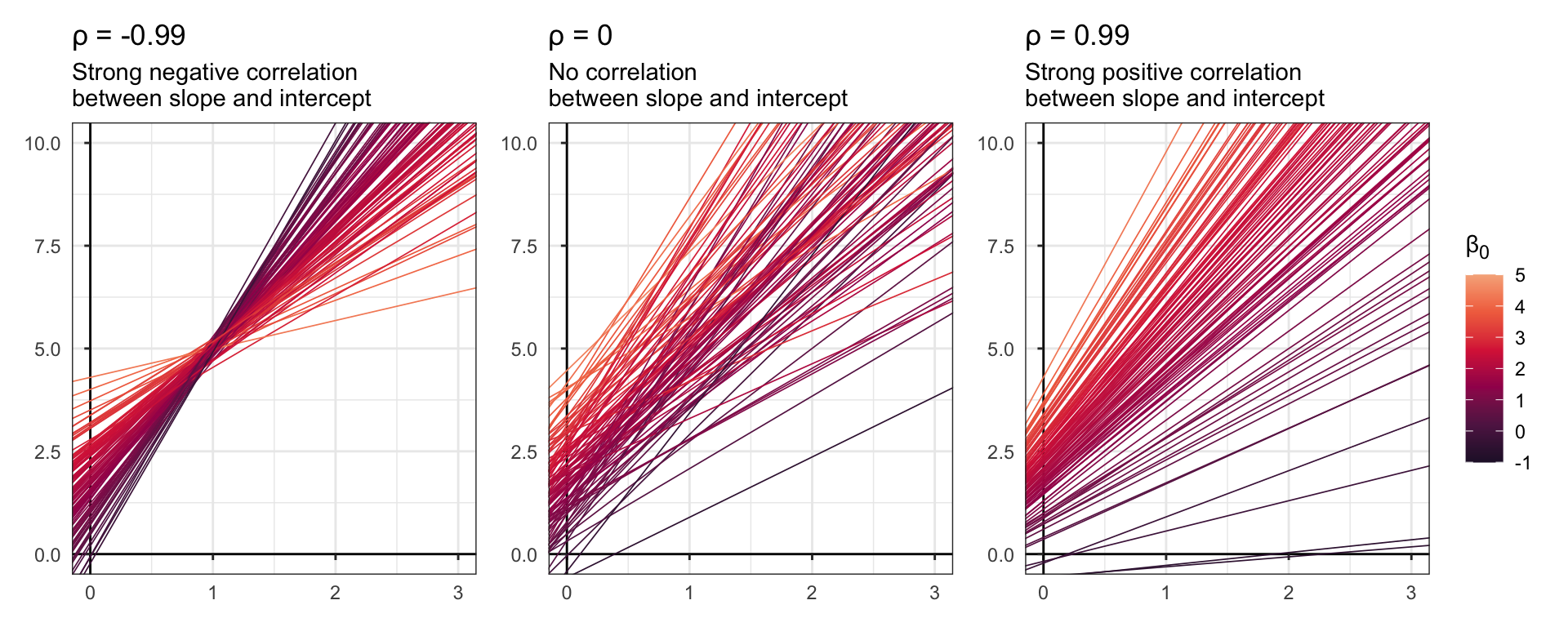
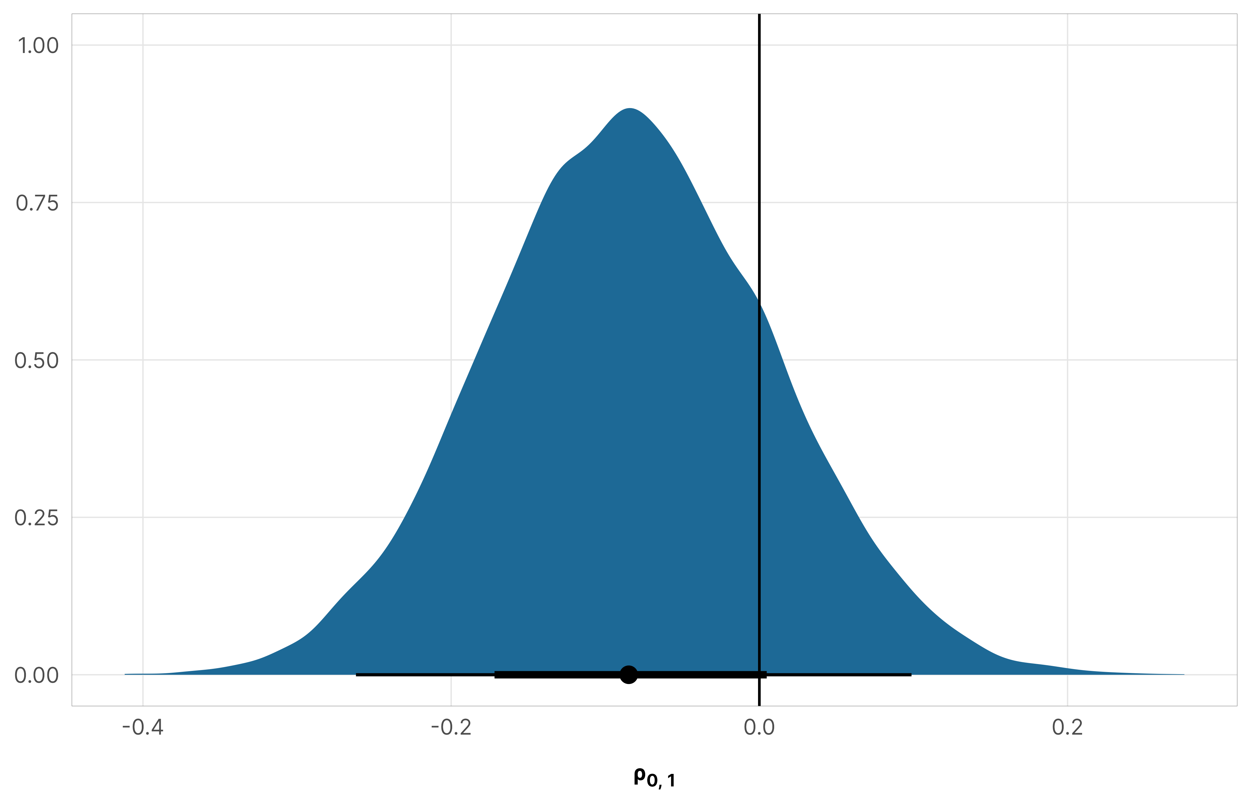
Due to the magic of multilevel models, these intercept and slope offsets are actually correlated with each other—we modeled the offsets from a multivariate normal distribution, and the correlation between the two $b_{n_j}$ parameters is defined by $\rho_{0, 1}$:

\[ \left( \begin{array}{c} b_{0_j} \\ b_{1_j} \end{array} \right) \sim \text{MV}\,\mathcal{N} \left[ \left( \begin{array}{c} 0 \\ 0 \\ \end{array} \right) , \, \left( \begin{array}{cc} \sigma^2_{0} & {\color{red} \rho_{0, 1}}\, \sigma_{0} \sigma_{1} \\ \cdots & \sigma^2_{1} \end{array} \right) \right] \]

Section 17.3 in Bayes Rules! illustrates what this correlation means in practice, and I made my own version of their plot here:

When $\rho$ is negative, bigger intercepts have smaller slopes; when $\rho$ is positive, bigger intercepts have bigger slopes. With our data, if $\rho$ is big and positive it would imply that countries with higher baseline levels of aid would see a larger and steeper year effect. In our actual model, $\rho$ is basically zero though:

Code

m_oda_prelim_time_only_total$model %>% 
  spread_draws(cor_gwcode__Intercept__year_c) %>% 
  ggplot(aes(x = cor_gwcode__Intercept__year_c)) +
  stat_halfeye(fill = clrs$Prism[2]) +
  geom_vline(xintercept = 0) +
  labs(x = "ρ<sub>0, 1</sub>", y = NULL) +
  theme_donors() +
  theme(axis.title.x = element_markdown())

Does this $\rho$ term have any practical application for the question we’re answering here? Not really. Is it super neat anyway? Yep.

Within- and between-country variability (σs)

Finally, we can look at all the $\sigma$ terms. We have three to work with:

$\sigma_y$ (sd__Observation): the variability of aid within countries. It’s 1.03, which means that within any country, their total ODA varies by 1 logged unit, so if their baseline is $e^{19}$, their outcome will bounce around between $e^{18}$ and $e^{20}$ over time.
$\sigma_0$ (sd__(Intercept) for the gwcode group): the variability between countries’ baseline averages, or the variability around the $b_{0_j}$ offsets. Here it’s 1.51, which means that across or between countries, total ODA varies by 1.5 logged units.
$\sigma_1$ (sd__year_c for the gwcode group): the variability between countries’ year effects, or the variability around the $b_{1_j}$ offsets. Here it’s 0.08, which means that average year effects vary by 8ish% across or between countries.

Code

m_oda_prelim_time_only_total$model %>% 
  tidy(effects = "ran_pars") %>% 
  select(-component, -effect) %>% 
  filter(!str_starts(term, "cor"))
## # A tibble: 3 × 6
##   group    term            estimate std.error conf.low conf.high
##   <chr>    <chr>              <dbl>     <dbl>    <dbl>     <dbl>
## 1 gwcode   sd__(Intercept)   1.51     0.0937    1.34      1.70  
## 2 gwcode   sd__year_c        0.0847   0.00632   0.0732    0.0979
## 3 Residual sd__Observation   1.03     0.0138    1.00      1.06

For whatever reason, we can’t get an ICC for the percent of variation explained by between-country differences:

Code

performance::icc(m_oda_prelim_time_only_total$model)
## [1] NA

We can use performance::variance_decomposition() to get a comparable number, since it uses the posterior predictive distribution of the model to figure out the between-country variance. It looks like between-country differences explain like 97% of the variation in ODA? Maybe that’s true, or maybe that’s an artifact of the WEIRDLY MASSIVE variance values it calculated here (the difference in variances is in the quintillions!). idk.

Code

performance::variance_decomposition(m_oda_prelim_time_only_total$model)
## # Random Effect Variances and ICC
## 
## Conditioned on: all random effects
## 
## ## Variance Ratio (comparable to ICC)
## Ratio: 0.97  CI 95%: [0.93 0.99]
## 
## ## Variances of Posterior Predicted Distribution
## Conditioned on fixed effects:   852776255087778048.00  CI 95%: [  472418355353042944.00  1633097449873477376.00]
## Conditioned on rand. effects: 28350410596168671232.00  CI 95%: [16026107771162734592.00 89196474994505465856.00]
## 
## ## Difference in Variances
## Difference: 27452860054043279360.00  CI 95%: [15096287018349314048.00 88040877640079458304.00]

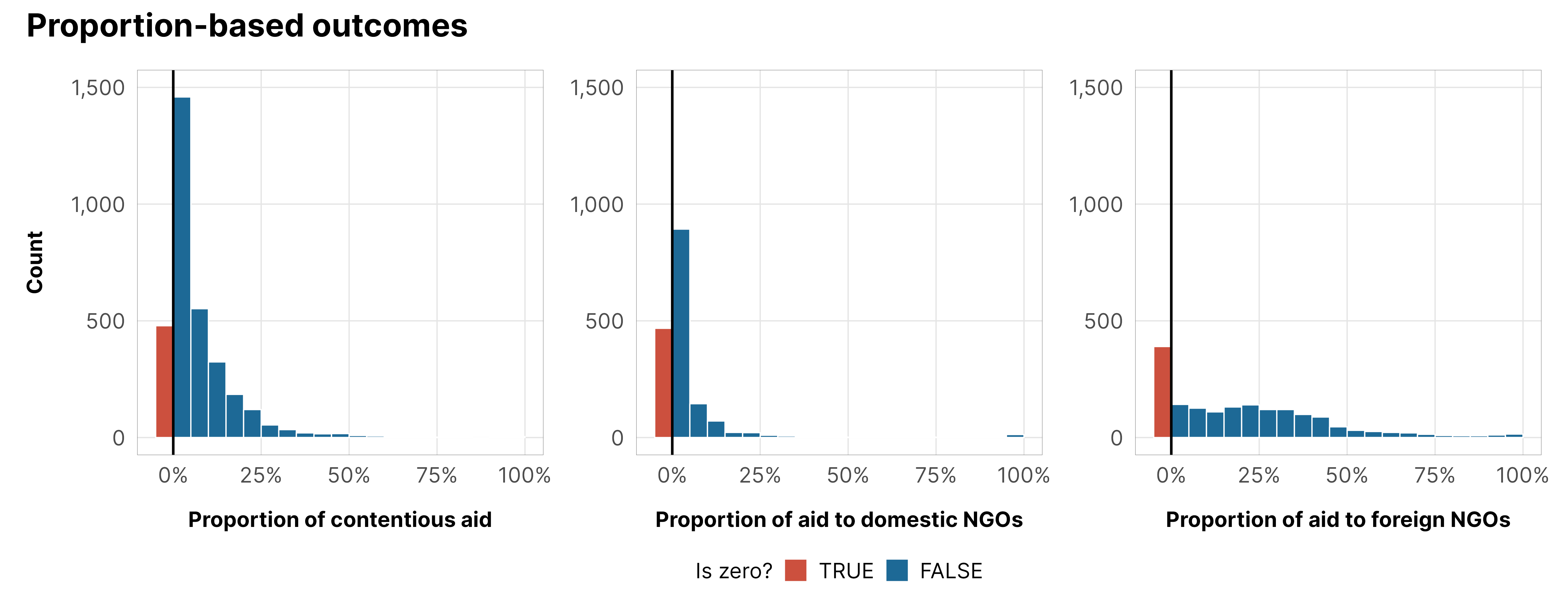
Zero-inflated models (proportions)

Our different proportion variables also have a substantial number of zeros:

Code

df_country_aid_laws %>% 
  mutate(prop_contentious = ifelse(prop_contentious == 0, -0.05, prop_contentious)) %>% 
  ggplot(aes(x = year, y = prop_contentious)) +
  geom_line(aes(group = country), linewidth = 0.075, alpha = 0.5) +
  stat_summary(geom = "line", fun = "mean", color = clrs$Prism[8], linewidth = 1.25) +
  geom_hline(yintercept = 0.001) +
  scale_y_continuous(labels = c("Exactly 0%", ">0%", "25%", "50%", "75%", "100%"), 
                     breaks = c(-0.05, 0.001, 0.25, 0.5, 0.75, 1)) +
  labs(x = NULL, y = "Proportion of contentious aid", color = NULL) +
  theme_donors()

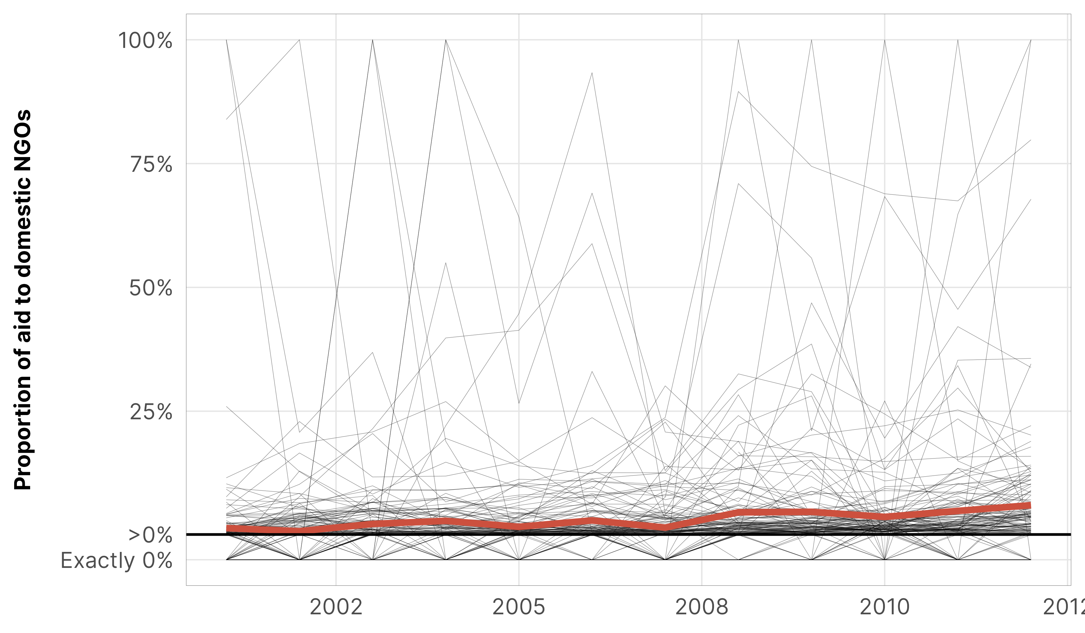
Code

df_country_aid_usaid %>% 
  mutate(prop_ngo_dom = ifelse(prop_ngo_dom == 0, -0.05, prop_ngo_dom)) %>% 
  ggplot(aes(x = year, y = prop_ngo_dom)) +
  geom_line(aes(group = country), linewidth = 0.075, alpha = 0.5) +
  stat_summary(geom = "line", fun = "mean", color = clrs$Prism[8], linewidth = 1.25) +
  geom_hline(yintercept = 0.001) +
  scale_y_continuous(labels = c("Exactly 0%", ">0%", "25%", "50%", "75%", "100%"), 
                     breaks = c(-0.05, 0.001, 0.25, 0.5, 0.75, 1)) +
  labs(x = NULL, y = "Proportion of aid to domestic NGOs", color = NULL) +
  theme_donors()

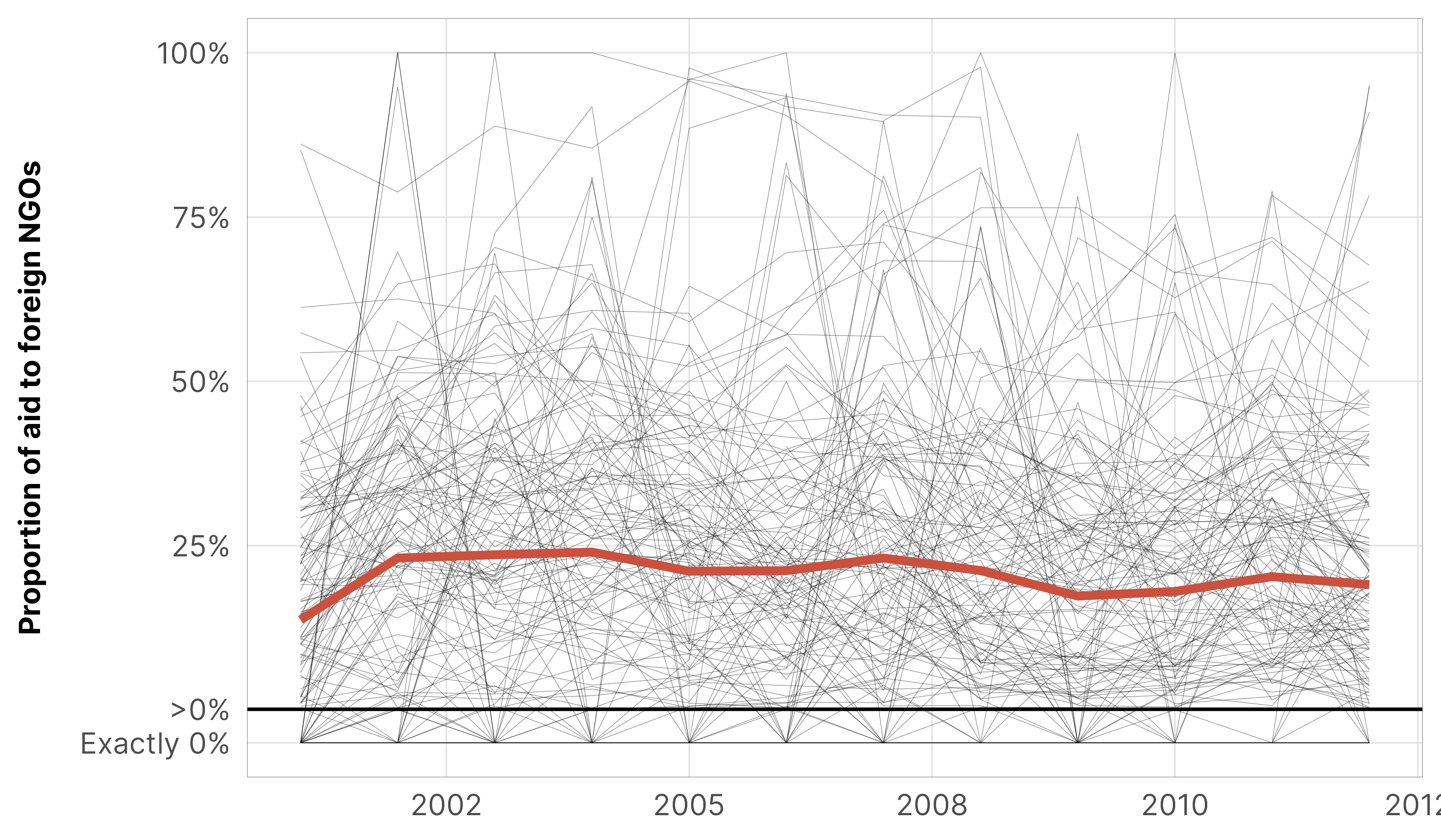
Code

df_country_aid_usaid %>% 
  mutate(prop_ngo_foreign = ifelse(prop_ngo_foreign == 0, -0.05, prop_ngo_foreign)) %>% 
  ggplot(aes(x = year, y = prop_ngo_foreign)) +
  geom_line(aes(group = country), linewidth = 0.075, alpha = 0.5) +
  stat_summary(geom = "line", fun = "mean", color = clrs$Prism[8], linewidth = 1.25) +
  geom_hline(yintercept = 0.001) +
  scale_y_continuous(labels = c("Exactly 0%", ">0%", "25%", "50%", "75%", "100%"), 
                     breaks = c(-0.05, 0.001, 0.25, 0.5, 0.75, 1)) +
  labs(x = NULL, y = "Proportion of aid to foreign NGOs", color = NULL) +
  theme_donors()

As with total aid, we’re not entirely sure what the underlying zero inflation process looks like for the different proportion variables we care about. For the proportion of contentious aid there’s a definite parabolic time trend, similar to what we saw with the hurdled model of ODA.

Code

df_country_aid_laws %>% 
  group_by(year) %>% 
  summarize(prop_zero = mean(prop_contentious == 0)) %>% 
  ggplot(aes(x = year, y = prop_zero)) +
  geom_line(linewidth = 0.5, color = "grey70") +
  geom_point(size = 1) + 
  geom_smooth(aes(color = "y = x"), method = "lm", 
              formula = y ~ x, se = FALSE) +
  geom_smooth(aes(color = "y = x + x<sup>2</sup>"), method = "lm", 
              formula = y ~ x + I(x^2), se = FALSE) +
  scale_y_continuous(labels = label_percent()) +
  scale_color_manual(values = clrs$Prism[c(3, 11)]) +
  labs(x = NULL, y = "Proportion of countries\nwith zero contentious aid",
       color = NULL) +
  theme_donors() +
  theme(legend.text = element_markdown())

Formal statistical model

To account for this underlying zero-inflation process, we’ll use a zero-inflated beta family with a multilevel hierarchical model with country-specific intercepts and a year trend with country-specific offsets (again following best practices for working with panel data with multilevel models). Earlier we didn’t include any polynomials to make it easier to interpret things. Here, for the sake of practice and illustration, we will add a squared term for year. As before, we center the year at 2000, and we’ll just look at the effect of year on contentious aid, since this is just a general illustration of how to work with these models.

In {brms}’s random effects syntax, the model formula looks like this:

Code

bf(prop_contentious ~ year_c + (1 + year_c | gwcode),
   zi ~ year_c + I(year_c^2))

Equation 2 shows this in more formal mathematical notation, with all the different random effects offsets and priors all working together simultaneously:

\[ \begin{aligned} & \mathrlap{\textbf{Zero-inflated model of proportion $i$ across time $t$ within each country $j$}} \\ \text{Proportion}_{it_j} &\sim \operatorname{Zero-inflated\, Beta}(\pi_{it}, \mu_{it_j}, \phi_y) \\ \\ & \textbf{Models for distribution parameters} \\ \operatorname{logit}(\pi_{it}) &= \gamma_0 + \gamma_1 \text{Year}_{it} + \gamma_2 \text{Year}^2_{it} & \text{Zero/not-zero process} \\[4pt] \operatorname{logit}(\mu_{it_j}) &= (\beta_0 + b_{0_j}) + (\beta_1 + b_{1_j}) \text{Year}_{it_j} & \text{Within-country variation} \\[4pt] \left( \begin{array}{c} b_{0_j} \\ b_{1_j} \end{array} \right) &\sim \text{MV}\,\mathcal{N} \left[ \left( \begin{array}{c} 0 \\ 0 \\ \end{array} \right) , \, \left( \begin{array}{cc} \sigma^2_{0} & \rho_{0, 1}\, \sigma_{0} \sigma_{1} \\ \cdots & \sigma^2_{1} \end{array} \right) \right] & \text{Variability in average intercepts and slopes} \\ \\ & \textbf{Priors} \\ \gamma_0 &\sim \text{Student $t$}(3, 0, 1.5) & \text{Prior for intercept in hurdle model} \\ \gamma_1, \gamma_2 &\sim \text{Student $t$}(3, 0, 1.5) & \text{Prior for year effect in hurdle model} \\ \beta_0 &\sim \text{Student $t$}(3, 0, 1.5) & \text{Prior for global average proportion} \\ \beta_1 &\sim \text{Student $t$}(3, 0, 1.5) & \text{Prior for global year effect} \\ \phi_y &\sim \operatorname{Exponential}(1) & \text{Prior for within-country variability} \\ \sigma_0 &\sim \operatorname{Exponential}(1) & \text{Prior for between-country intercept variability} \\ \sigma_1 &\sim \operatorname{Exponential}(1) & \text{Prior for between-country slope variability} \\ \rho &\sim \operatorname{LKJ}(2) & \text{Prior for between-country variability} \end{aligned} \tag{2}\]

Prior simulation

For this year-and-country-only model, we set the following priors:

Code

design <- "
  AAABBB
  CCCDDD
  EEFFGG
"

m_purpose_prelim_time_only_total$priors %>% 
  parse_dist() %>% 
  # K = dimension of correlation matrix; 
  # ours is 2x2 here because we have one random slope
  marginalize_lkjcorr(K = 2) %>%
  mutate(nice_title = glue::glue("**{class}**: {prior}"),
         stage = ifelse(dpar == "zi", "Zero-inflated part (π)", "Beta part (µ and φ)")) %>% 
  mutate(nice_title = fct_inorder(nice_title),
         stage = fct_rev(fct_inorder(stage))) %>% 
  ggplot(aes(y = 0, dist = .dist, args = .args, fill = prior)) +
  stat_slab(normalize = "panels") +
  scale_fill_manual(values = clrs$Prism[c(1, 2, 5)]) +
  facet_manual(vars(stage, nice_title), design = design, scales = "free_x",
               strip = strip_nested(background_x = list(element_rect(fill = "grey92"), NULL),
                                    by_layer_x = TRUE)) +
  guides(fill = "none") +
  labs(x = NULL, y = NULL) +
  theme_donors(prior = TRUE) +
  theme(strip.text = element_markdown())

As we did with the hurdle model, we’ll simulate from the prior distributions to make sure these are reasonable-ish. These are kind of neat. Some simulated countries have a good range of contentious aid over time; others jump between 0% and 100% pretty rapidly (which also happens in the real data). These priors are fine enough.

Code

df_country_aid_laws %>%  
  add_epred_draws(m_purpose_prelim_time_only_total$model_prior_only, ndraws = 9,
                  seed = 12345) %>% 
  mutate(year = year_c + 2000) %>% 
  ggplot(aes(x = year, y = .epred, group = paste(gwcode, .draw))) +
  geom_line(linewidth = 0.15, color = clrs$Prism[8]) +
  scale_y_continuous(labels = label_percent()) +
  facet_wrap(vars(.draw)) +
  labs(x = "Year", y = "Percent of contentious aid", title = "Results sampled from prior only",
       subtitle = "Each panel shows plausible aid-year relationships for 142 simulated countries") +
  theme_donors()

Posterior checks

MCMC diagnostics

Code

m_purpose_prelim_time_only_total$model %>% 
  gather_draws(`^b_.*|^sd_.*|^cor_.*|^phi`, regex = TRUE) %>% 
  ggplot(aes(x = .iteration, y = .value, color = factor(.chain))) +
  geom_line(size = 0.1) +
  scale_color_manual(values = clrs$Sunset[3:6]) +
  facet_wrap(vars(.variable), scales = "free_y") +
  theme_donors()

Code

m_purpose_prelim_time_only_total$model %>% 
  gather_draws(`^b_.*|^sd_.*|^cor_.*|^phi`, regex = TRUE) %>% 
  group_by(.variable) %>% 
  mutate(draw_rank = rank(.value)) %>% 
  ggplot(aes(x = draw_rank, color = factor(.chain))) +
  stat_bin(geom = "step", binwidth = 500, position = position_identity(), boundary = 0) +
  scale_color_manual(values = clrs$Sunset[3:6]) +
  facet_wrap(vars(.variable), scales = "free_y") +
  theme_donors() +
  theme(axis.text.y = element_blank(), axis.title.y = element_blank(), axis.ticks.y = element_blank())

Code

rstan::get_elapsed_time(m_purpose_prelim_time_only_total$model$fit)
##         warmup sample
## chain:1   94.8  100.3
## chain:2   97.6   53.6
## chain:3   99.8   58.3
## chain:4   96.5   53.6

rstan::get_elapsed_time(m_purpose_prelim_time_only_total$model$fit) %>% 
  as.data.frame() %>% 
  summarize(longest = lubridate::as.duration(max(warmup + sample)))
##                    longest
## 1 195.157s (~3.25 minutes)

Posterior predictive check

It’s so beautiful!

Code

withr::with_seed(1234, {
  pp_check(m_purpose_prelim_time_only_total$model, ndraws = 20) +
    labs(x = "Percent of contentious aid", 
         title = "Zero-inflated beta model posterior predictive check") +
    scale_x_continuous(labels = label_percent()) +
    theme_donors()
})

Analyzing the posterior

Though we only really care about one effect here, we actually have a ton of different parameters to work with—301!

Show the full list of 301 things

get_variables(m_purpose_prelim_time_only_total$model)
##   [1] "b_Intercept"                   "b_zi_Intercept"                "b_zi_year_c"                  
##   [4] "b_zi_Iyear_cE2"                "b_year_c"                      "sd_gwcode__Intercept"         
##   [7] "sd_gwcode__year_c"             "cor_gwcode__Intercept__year_c" "phi"                          
##  [10] "r_gwcode[40,Intercept]"        "r_gwcode[41,Intercept]"        "r_gwcode[42,Intercept]"       
##  [13] "r_gwcode[51,Intercept]"        "r_gwcode[52,Intercept]"        "r_gwcode[70,Intercept]"       
##  [16] "r_gwcode[90,Intercept]"        "r_gwcode[91,Intercept]"        "r_gwcode[92,Intercept]"       
##  [19] "r_gwcode[93,Intercept]"        "r_gwcode[94,Intercept]"        "r_gwcode[95,Intercept]"       
##  [22] "r_gwcode[100,Intercept]"       "r_gwcode[101,Intercept]"       "r_gwcode[110,Intercept]"      
##  [25] "r_gwcode[130,Intercept]"       "r_gwcode[135,Intercept]"       "r_gwcode[140,Intercept]"      
##  [28] "r_gwcode[145,Intercept]"       "r_gwcode[150,Intercept]"       "r_gwcode[155,Intercept]"      
##  [31] "r_gwcode[160,Intercept]"       "r_gwcode[165,Intercept]"       "r_gwcode[235,Intercept]"      
##  [34] "r_gwcode[290,Intercept]"       "r_gwcode[310,Intercept]"       "r_gwcode[316,Intercept]"      
##  [37] "r_gwcode[317,Intercept]"       "r_gwcode[339,Intercept]"       "r_gwcode[341,Intercept]"      
##  [40] "r_gwcode[343,Intercept]"       "r_gwcode[344,Intercept]"       "r_gwcode[345,Intercept]"      
##  [43] "r_gwcode[346,Intercept]"       "r_gwcode[347,Intercept]"       "r_gwcode[349,Intercept]"      
##  [46] "r_gwcode[352,Intercept]"       "r_gwcode[355,Intercept]"       "r_gwcode[359,Intercept]"      
##  [49] "r_gwcode[360,Intercept]"       "r_gwcode[365,Intercept]"       "r_gwcode[366,Intercept]"      
##  [52] "r_gwcode[367,Intercept]"       "r_gwcode[368,Intercept]"       "r_gwcode[369,Intercept]"      
##  [55] "r_gwcode[370,Intercept]"       "r_gwcode[371,Intercept]"       "r_gwcode[372,Intercept]"      
##  [58] "r_gwcode[373,Intercept]"       "r_gwcode[404,Intercept]"       "r_gwcode[411,Intercept]"      
##  [61] "r_gwcode[420,Intercept]"       "r_gwcode[432,Intercept]"       "r_gwcode[433,Intercept]"      
##  [64] "r_gwcode[434,Intercept]"       "r_gwcode[435,Intercept]"       "r_gwcode[436,Intercept]"      
##  [67] "r_gwcode[437,Intercept]"       "r_gwcode[438,Intercept]"       "r_gwcode[439,Intercept]"      
##  [70] "r_gwcode[450,Intercept]"       "r_gwcode[451,Intercept]"       "r_gwcode[452,Intercept]"      
##  [73] "r_gwcode[461,Intercept]"       "r_gwcode[471,Intercept]"       "r_gwcode[475,Intercept]"      
##  [76] "r_gwcode[481,Intercept]"       "r_gwcode[482,Intercept]"       "r_gwcode[484,Intercept]"      
##  [79] "r_gwcode[490,Intercept]"       "r_gwcode[500,Intercept]"       "r_gwcode[501,Intercept]"      
##  [82] "r_gwcode[510,Intercept]"       "r_gwcode[516,Intercept]"       "r_gwcode[517,Intercept]"      
##  [85] "r_gwcode[520,Intercept]"       "r_gwcode[522,Intercept]"       "r_gwcode[530,Intercept]"      
##  [88] "r_gwcode[531,Intercept]"       "r_gwcode[540,Intercept]"       "r_gwcode[541,Intercept]"      
##  [91] "r_gwcode[551,Intercept]"       "r_gwcode[552,Intercept]"       "r_gwcode[553,Intercept]"      
##  [94] "r_gwcode[560,Intercept]"       "r_gwcode[565,Intercept]"       "r_gwcode[570,Intercept]"      
##  [97] "r_gwcode[571,Intercept]"       "r_gwcode[572,Intercept]"       "r_gwcode[580,Intercept]"      
## [100] "r_gwcode[581,Intercept]"       "r_gwcode[590,Intercept]"       "r_gwcode[600,Intercept]"      
## [103] "r_gwcode[615,Intercept]"       "r_gwcode[616,Intercept]"       "r_gwcode[620,Intercept]"      
## [106] "r_gwcode[625,Intercept]"       "r_gwcode[626,Intercept]"       "r_gwcode[630,Intercept]"      
## [109] "r_gwcode[640,Intercept]"       "r_gwcode[645,Intercept]"       "r_gwcode[651,Intercept]"      
## [112] "r_gwcode[652,Intercept]"       "r_gwcode[660,Intercept]"       "r_gwcode[663,Intercept]"      
## [115] "r_gwcode[666,Intercept]"       "r_gwcode[670,Intercept]"       "r_gwcode[678,Intercept]"      
## [118] "r_gwcode[690,Intercept]"       "r_gwcode[692,Intercept]"       "r_gwcode[694,Intercept]"      
## [121] "r_gwcode[696,Intercept]"       "r_gwcode[698,Intercept]"       "r_gwcode[700,Intercept]"      
## [124] "r_gwcode[701,Intercept]"       "r_gwcode[702,Intercept]"       "r_gwcode[703,Intercept]"      
## [127] "r_gwcode[704,Intercept]"       "r_gwcode[705,Intercept]"       "r_gwcode[710,Intercept]"      
## [130] "r_gwcode[712,Intercept]"       "r_gwcode[731,Intercept]"       "r_gwcode[732,Intercept]"      
## [133] "r_gwcode[750,Intercept]"       "r_gwcode[760,Intercept]"       "r_gwcode[770,Intercept]"      
## [136] "r_gwcode[771,Intercept]"       "r_gwcode[775,Intercept]"       "r_gwcode[780,Intercept]"      
## [139] "r_gwcode[790,Intercept]"       "r_gwcode[800,Intercept]"       "r_gwcode[811,Intercept]"      
## [142] "r_gwcode[812,Intercept]"       "r_gwcode[816,Intercept]"       "r_gwcode[820,Intercept]"      
## [145] "r_gwcode[830,Intercept]"       "r_gwcode[840,Intercept]"       "r_gwcode[850,Intercept]"      
## [148] "r_gwcode[860,Intercept]"       "r_gwcode[910,Intercept]"       "r_gwcode[940,Intercept]"      
## [151] "r_gwcode[950,Intercept]"       "r_gwcode[40,year_c]"           "r_gwcode[41,year_c]"          
## [154] "r_gwcode[42,year_c]"           "r_gwcode[51,year_c]"           "r_gwcode[52,year_c]"          
## [157] "r_gwcode[70,year_c]"           "r_gwcode[90,year_c]"           "r_gwcode[91,year_c]"          
## [160] "r_gwcode[92,year_c]"           "r_gwcode[93,year_c]"           "r_gwcode[94,year_c]"          
## [163] "r_gwcode[95,year_c]"           "r_gwcode[100,year_c]"          "r_gwcode[101,year_c]"         
## [166] "r_gwcode[110,year_c]"          "r_gwcode[130,year_c]"          "r_gwcode[135,year_c]"         
## [169] "r_gwcode[140,year_c]"          "r_gwcode[145,year_c]"          "r_gwcode[150,year_c]"         
## [172] "r_gwcode[155,year_c]"          "r_gwcode[160,year_c]"          "r_gwcode[165,year_c]"         
## [175] "r_gwcode[235,year_c]"          "r_gwcode[290,year_c]"          "r_gwcode[310,year_c]"         
## [178] "r_gwcode[316,year_c]"          "r_gwcode[317,year_c]"          "r_gwcode[339,year_c]"         
## [181] "r_gwcode[341,year_c]"          "r_gwcode[343,year_c]"          "r_gwcode[344,year_c]"         
## [184] "r_gwcode[345,year_c]"          "r_gwcode[346,year_c]"          "r_gwcode[347,year_c]"         
## [187] "r_gwcode[349,year_c]"          "r_gwcode[352,year_c]"          "r_gwcode[355,year_c]"         
## [190] "r_gwcode[359,year_c]"          "r_gwcode[360,year_c]"          "r_gwcode[365,year_c]"         
## [193] "r_gwcode[366,year_c]"          "r_gwcode[367,year_c]"          "r_gwcode[368,year_c]"         
## [196] "r_gwcode[369,year_c]"          "r_gwcode[370,year_c]"          "r_gwcode[371,year_c]"         
## [199] "r_gwcode[372,year_c]"          "r_gwcode[373,year_c]"          "r_gwcode[404,year_c]"         
## [202] "r_gwcode[411,year_c]"          "r_gwcode[420,year_c]"          "r_gwcode[432,year_c]"         
## [205] "r_gwcode[433,year_c]"          "r_gwcode[434,year_c]"          "r_gwcode[435,year_c]"         
## [208] "r_gwcode[436,year_c]"          "r_gwcode[437,year_c]"          "r_gwcode[438,year_c]"         
## [211] "r_gwcode[439,year_c]"          "r_gwcode[450,year_c]"          "r_gwcode[451,year_c]"         
## [214] "r_gwcode[452,year_c]"          "r_gwcode[461,year_c]"          "r_gwcode[471,year_c]"         
## [217] "r_gwcode[475,year_c]"          "r_gwcode[481,year_c]"          "r_gwcode[482,year_c]"         
## [220] "r_gwcode[484,year_c]"          "r_gwcode[490,year_c]"          "r_gwcode[500,year_c]"         
## [223] "r_gwcode[501,year_c]"          "r_gwcode[510,year_c]"          "r_gwcode[516,year_c]"         
## [226] "r_gwcode[517,year_c]"          "r_gwcode[520,year_c]"          "r_gwcode[522,year_c]"         
## [229] "r_gwcode[530,year_c]"          "r_gwcode[531,year_c]"          "r_gwcode[540,year_c]"         
## [232] "r_gwcode[541,year_c]"          "r_gwcode[551,year_c]"          "r_gwcode[552,year_c]"         
## [235] "r_gwcode[553,year_c]"          "r_gwcode[560,year_c]"          "r_gwcode[565,year_c]"         
## [238] "r_gwcode[570,year_c]"          "r_gwcode[571,year_c]"          "r_gwcode[572,year_c]"         
## [241] "r_gwcode[580,year_c]"          "r_gwcode[581,year_c]"          "r_gwcode[590,year_c]"         
## [244] "r_gwcode[600,year_c]"          "r_gwcode[615,year_c]"          "r_gwcode[616,year_c]"         
## [247] "r_gwcode[620,year_c]"          "r_gwcode[625,year_c]"          "r_gwcode[626,year_c]"         
## [250] "r_gwcode[630,year_c]"          "r_gwcode[640,year_c]"          "r_gwcode[645,year_c]"         
## [253] "r_gwcode[651,year_c]"          "r_gwcode[652,year_c]"          "r_gwcode[660,year_c]"         
## [256] "r_gwcode[663,year_c]"          "r_gwcode[666,year_c]"          "r_gwcode[670,year_c]"         
## [259] "r_gwcode[678,year_c]"          "r_gwcode[690,year_c]"          "r_gwcode[692,year_c]"         
## [262] "r_gwcode[694,year_c]"          "r_gwcode[696,year_c]"          "r_gwcode[698,year_c]"         
## [265] "r_gwcode[700,year_c]"          "r_gwcode[701,year_c]"          "r_gwcode[702,year_c]"         
## [268] "r_gwcode[703,year_c]"          "r_gwcode[704,year_c]"          "r_gwcode[705,year_c]"         
## [271] "r_gwcode[710,year_c]"          "r_gwcode[712,year_c]"          "r_gwcode[731,year_c]"         
## [274] "r_gwcode[732,year_c]"          "r_gwcode[750,year_c]"          "r_gwcode[760,year_c]"         
## [277] "r_gwcode[770,year_c]"          "r_gwcode[771,year_c]"          "r_gwcode[775,year_c]"         
## [280] "r_gwcode[780,year_c]"          "r_gwcode[790,year_c]"          "r_gwcode[800,year_c]"         
## [283] "r_gwcode[811,year_c]"          "r_gwcode[812,year_c]"          "r_gwcode[816,year_c]"         
## [286] "r_gwcode[820,year_c]"          "r_gwcode[830,year_c]"          "r_gwcode[840,year_c]"         
## [289] "r_gwcode[850,year_c]"          "r_gwcode[860,year_c]"          "r_gwcode[910,year_c]"         
## [292] "r_gwcode[940,year_c]"          "r_gwcode[950,year_c]"          "lprior"                       
## [295] "lp__"                          "accept_stat__"                 "treedepth__"                  
## [298] "stepsize__"                    "divergent__"                   "n_leapfrog__"                 
## [301] "energy__"

142 country-specific intercept offsets: $b_{0_j}$
142 country-specific offsets to the year_c slope: $b_{1_j}$
2 global terms (intercept and year_c) for the $\mu$ part of the model: $\beta_0$ and $\beta_1$
3 global terms (intercept, year_c, and year_c_E2) for the zero-inflated $\pi$ part of the model: $\gamma_0$ and $\gamma_1$
The overall within-country $\phi$: $\phi_y$
The variability in country-specific intercept and slope offsets: $\sigma^2_0$ and $\sigma^2_1$
The correlation between country-specific slopes and intercepts: $\rho$
8 auxiliary Stan-specific things like lprior, n_leapfrog__, energy__, etc.

Code

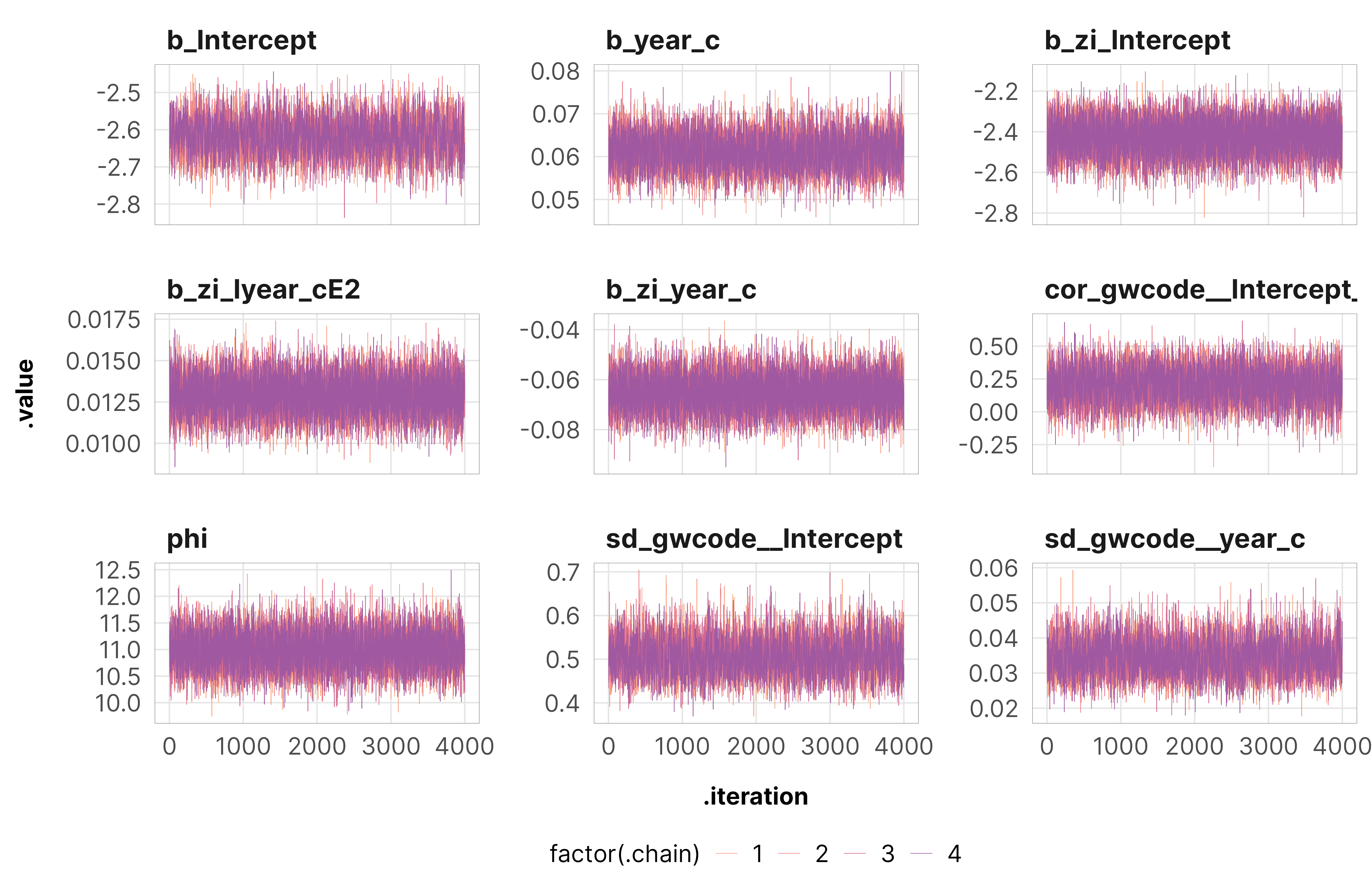
m_purpose_prelim_time_only_total$model
##  Family: zero_inflated_beta 
##   Links: mu = logit; phi = identity; zi = logit 
## Formula: prop_contentious_trunc ~ year_c + (1 + year_c | gwcode) 
##          zi ~ year_c + I(year_c^2)
##    Data: dat (Number of observations: 3293) 
##   Draws: 4 chains, each with iter = 5000; warmup = 1000; thin = 1;
##          total post-warmup draws = 16000
## 
## Group-Level Effects: 
## ~gwcode (Number of levels: 142) 
##                       Estimate Est.Error l-95% CI u-95% CI Rhat Bulk_ESS Tail_ESS
## sd(Intercept)             0.51      0.04     0.43     0.60 1.00     3773     6609
## sd(year_c)                0.03      0.01     0.03     0.05 1.00     3499     6555
## cor(Intercept,year_c)     0.21      0.13    -0.06     0.46 1.00     6667     9619
## 
## Population-Level Effects: 
##              Estimate Est.Error l-95% CI u-95% CI Rhat Bulk_ESS Tail_ESS
## Intercept       -2.62      0.05    -2.72    -2.52 1.00     3019     5759
## zi_Intercept    -2.43      0.09    -2.60    -2.26 1.00    18250    12967
## zi_year_c       -0.07      0.01    -0.08    -0.05 1.00    22613    12673
## zi_Iyear_cE2     0.01      0.00     0.01     0.02 1.00    17721    13086
## year_c           0.06      0.00     0.05     0.07 1.00     7034     9936
## 
## Family Specific Parameters: 
##     Estimate Est.Error l-95% CI u-95% CI Rhat Bulk_ESS Tail_ESS
## phi    10.99      0.35    10.33    11.68 1.00    13480    11770
## 
## Draws were sampled using sample(hmc). For each parameter, Bulk_ESS
## and Tail_ESS are effective sample size measures, and Rhat is the potential
## scale reduction factor on split chains (at convergence, Rhat = 1).

As we did with the hurdle model previously, we’ll walk through all these different population-level (or global within-country) effects, group level (between-country) effects, and within- and between-country variability. We’ll also look at effects at each part of the model—the regular part that models $\mu$ and the zero-inflated part that models $\pi$.

Non-zero-inflated vs. zero-inflated parts (µ vs. π)

Like the hurdled model, we have three different parts of the model to work with:

\[ \begin{aligned} \text{Proportion}_{it_j} &\sim \operatorname{Zero-inflated\, Beta}(\pi_{it}, \mu_{it_j}, \phi_y) & \text{Proportion} \\ \operatorname{logit}(\pi_{it}) &= \gamma_0 + \gamma_1 \text{Year}_{it} + \gamma_2 \text{Year}^2_{it} & \text{on/off process} \\ \operatorname{logit}(\mu_{it_j}) &= (\beta_0 + b_{0_j}) + (\beta_1 + b_{1_j}) \text{Year}_{it_j} & \text{$\geq 0$ process} \end{aligned} \]

And like we did with the hurdle model previously (and like I illustrate in my guide here), we can use different combinations of linpred_draws(), epred_draws(), and predicted_draws() to explore different aspects of these parts’ posterior distributions.

Zero part (π and γs)

First we’ll look at the on/off process, or $\operatorname{logit}(\pi_{it})$. This is conceptually different from the hurdle process, which predicts if an outcome is 0 or not 0. With zero-inflation, we’re predicting if the data-generating process is on or not—but the data-generating process can still result in 0s, theoretically. Recall the monk example from Statistical Rethinking mentioned above—monks could transcribe 0 manuscripts because the whole transcription process is “off” and they do no work, or they could transcribe 0 manuscripts because they work really really slowly or are lazy, etc.

In this part of model, we used year and year², so we have a $\gamma_0$ coefficient for the intercept and $\gamma_1$ and $\gamma_2$ coefficients for the year effect. Theese are on the logit scale, so exponentiating them will give us an odds ratio, while inverse logit-ing them with plogis() will give us probabilities.

Importantly, because we’re working with polynomials, we can’t really just interpret the $\gamma_1$ and $\gamma_2$ year coefficients—they move together and influence the year effect simultaneously. They lead to a non-linear slope across the range of possible years. To see the year effect, then, we need to look at partial derivatives or marginal effects.

Here are the zero-inflated coefficients as log odds. We won’t exponentiate them because (1) an exponentiated value doesn’t make sense for an intercept, and (2) there are two year coefficients that work together, so we can’t interpret just one of the values.

Code

# Uninterpretable log odds
m_purpose_prelim_time_only_total$model %>% 
  tidy(effects = "fixed") %>% 
  filter(component == "zi")
## # A tibble: 3 × 7
##   effect component term        estimate std.error conf.low conf.high
##   <chr>  <chr>     <chr>          <dbl>     <dbl>    <dbl>     <dbl>
## 1 fixed  zi        (Intercept)  -2.43     0.0875   -2.60     -2.26  
## 2 fixed  zi        year_c       -0.0651   0.00727  -0.0793   -0.0508
## 3 fixed  zi        Iyear_cE2     0.0129   0.00115   0.0107    0.0152

To make the log odds intercept value (-2.62) more interpretable, we can convert it to a probability with $\frac{e^{\gamma_0}}{1 + e^{\gamma_0}}$, or plogis(), which is 0.068, which means that in the year 2000 (i.e. when year_c is 0), the model predicts that 6.8% of countries received 0 contentious aid.

We can confirm with a plot, which also helps set the stage for interpreting the year effect. In 2000 the predicted proportion is indeed 6.8%.

Code

plot_zi_zi <- m_purpose_prelim_time_only_total$model %>% 
  linpred_draws(newdata = tibble(year_c = seq(-10, 13, 1)),
                re_formula = NA,
                dpar = "zi", transform = TRUE) %>% 
  mutate(year = year_c + 2000) %>% 
  ggplot(aes(x = year, y = zi)) +
  stat_lineribbon(color = clrs$Emrld[7], alpha = 0.3) +
  scale_y_continuous(labels = label_percent()) +
  scale_fill_manual(values = clrs$Emrld[2:4]) +
  guides(fill = "none") +
  labs(x = NULL, y = "Predicted proportion\nof countries receiving\n0% contentious aid",
       subtitle = "Predicted global proportion of countries receiving 0% contentious aid, π only") +
  theme_donors()

plot_zi_zi_lines <- plot_zi_zi +
  geom_vline(xintercept = c(1992, 2000, 2010),
             linewidth = 0.25, linetype = "21")

plot_actual_zeros <- df_country_aid_laws %>% 
  group_by(year) %>% 
  summarize(prop_zero = sum(prop_contentious == 0) / n()) %>% 
  ggplot(aes(x = year, y = prop_zero)) + 
  geom_line(color = clrs$Emrld[5], linewidth = 1) +
  scale_y_continuous(labels = label_percent()) +
  labs(x = NULL, y = "Actual proportion of\ncountries receiving\n0% contentious aid",
       subtitle = "Actual global proportion of countries receiving 0% contentious aid") +
  theme_donors()

(plot_zi_zi_lines / plot_actual_zeros) &
  coord_cartesian(ylim = c(0, 0.45))

For the year effect, we need to look at the slope of the line at different years, since it changes across time. As seen in the plot, pre-2002ish, it’s a negative effect; after 2002ish, it’s positive.

Code

m_purpose_prelim_time_only_total$model %>% 
  marginaleffects(newdata = datagrid(year_c = c(-8, 0, 10)),
                  dpar = "zi") %>% 
  mutate(year = year_c + 2000) %>% 
  select(type, year_c, year, dydx, conf.low, conf.high, predicted)
##       type year_c year     dydx conf.low conf.high predicted
## 1 response     -8 1992 -0.05140 -0.06312  -0.04070    0.2537
## 2 response      0 2000 -0.00484 -0.00596  -0.00381    0.0813
## 3 response     10 2010  0.02374  0.01772   0.03038    0.1437

More precisely, in 1992 the year effect is -0.051, which means that one additional year is associated with a 5.14 percentage point decrease in the proportion of 0s, on average. In 2000, there is a tiny 0.484 percentage point decrease, while in 2010 there is a more substantial 2.374 increase in the proportion of 0s.

Non-zero part (µ and βs)

Next we’ll look at the part of the model that predicts what happens when the data-generating process is on (i.e. the monks are for sure working, so how many manuscripts will they transcribe?), or $\operatorname{logit}(\mu_{it_j})$. In this part of model, we only used year, so we have a $\beta_0$ coefficient for the intercept and a $\beta_1$ coefficient for the year effect. Since this is a beta model, the coefficients are on the logit scale, so we can exponentiate them or inverse logit them to make them more interpretable. As with the hurdle model example, technically we can’t interpret these $\beta$ coefficients directly because of the random effects, but we’ll pretend we can just for fun.

Code

# Log odds
# Uninterpretable log odds
m_purpose_prelim_time_only_total$model %>% 
  tidy(effects = "fixed") %>% 
  filter(component != "zi")
## # A tibble: 2 × 7
##   effect component term        estimate std.error conf.low conf.high
##   <chr>  <chr>     <chr>          <dbl>     <dbl>    <dbl>     <dbl>
## 1 fixed  cond      (Intercept)  -2.62     0.0495   -2.72     -2.52  
## 2 fixed  cond      year_c        0.0613   0.00410   0.0534    0.0694

# Exponentiated
m_purpose_prelim_time_only_total$model %>% 
  tidy(effects = "fixed") %>% 
  filter(component != "zi") %>% 
  mutate(across(c(estimate, conf.low, conf.high), exp))
## # A tibble: 2 × 7
##   effect component term        estimate std.error conf.low conf.high
##   <chr>  <chr>     <chr>          <dbl>     <dbl>    <dbl>     <dbl>
## 1 fixed  cond      (Intercept)   0.0729   0.0495    0.0660    0.0803
## 2 fixed  cond      year_c        1.06     0.00410   1.05      1.07

The intercept is nonsensical both as log odds and when exponentiated, but if we inverse logit its log odds with plogis(), we get 0.068, which means that in 2000, the predicted average proportion of contentious aid is 6.79%.

The exponentiated year effect is 1.063, which means that a one-year increase in time increases the likelihood of receiving additional contentious aid by 6.32%. BUT that’s (1) weird to think about as “receiving additional contentious aid”, and (2) wrong because of the multilevel nature of the model. So we won’t actually put much stock in these $\beta$ coefficients alone and save the more substantive interpretation of the year effect for the next section in this guide on conditional and marginal effects.

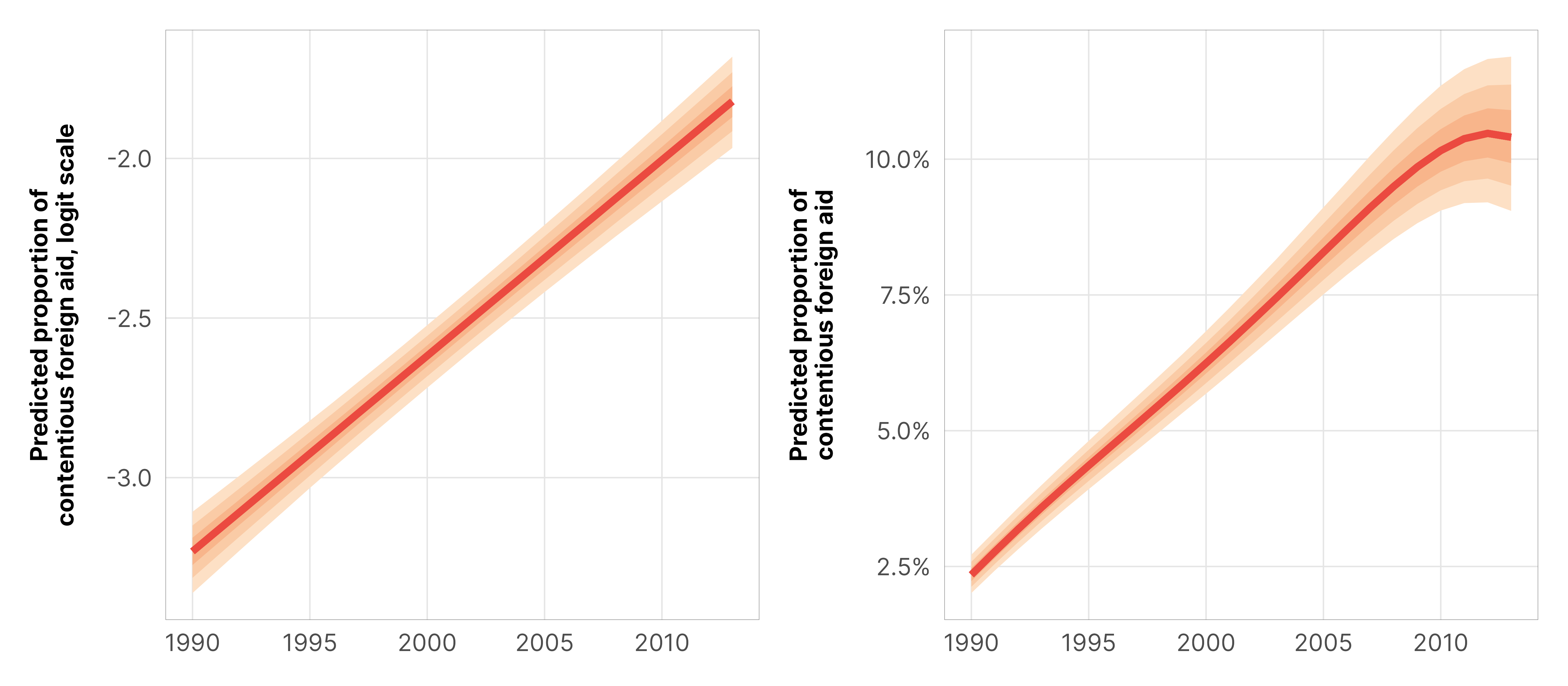
Instead of thinking about percent changes and log odds, we can look at predictions on the percentage point scale, which is far more intuitive. We can extract predictions from the $\operatorname{logit}(\mu_{it_j})$ part of the model with linpred_draws(). As before, with transform = FALSE we’ll get logit-scale values; with transform = TRUE we’ll get percentage points.

The predicted value in 2000 is 6.79%, as expected. The line goes up every year, also as expected. We don’t know how much it goes up at each year yet—we’re purposely holding off on finding the year effect until later so we can find conditional and marginal effects.

Code

plot_zi_mu_linpred <- m_purpose_prelim_time_only_total$model %>% 
  linpred_draws(newdata = tibble(year_c = seq(-10, 13, 1)),
                re_formula = NA, dpar = "mu") %>% 
  mutate(.linpred = exp(.linpred)) %>% 
  mutate(year = year_c + 2000) %>% 
  ggplot(aes(x = year, y = .linpred)) +
  stat_lineribbon(color = clrs$PurpOr[7], alpha = 0.3) +
  scale_y_continuous(labels = label_percent()) +
  scale_fill_manual(values = clrs$PurpOr[3:5]) +
  coord_cartesian(ylim = c(0, 0.20)) +
  guides(fill = "none") +
  labs(x = NULL, y = "Predicted percentage of\ncontentious aid",
       subtitle = "Predicted global average proportion of contentious aid, µ only") +
  theme_donors()
plot_zi_mu_linpred

Combined processes (y)

Finally, we can look at both parts of the model simultaneously. The outcome is a function of both the $\pi$ part and the $\mu$ part:

\[ \text{Proportion}_{it_j} \sim \operatorname{Zero-inflated\, Beta}(\pi_{it}, \mu_{it_j}, \phi_y) \] We can work with both of these parts at the same time if we epred_draws() instead of linpred_draws(), which calculates the expectation (the “e” in epred) of the posterior predictive distribution of the outcome, or $\textbf{E}(\text{Proportion}_{it_j})$.

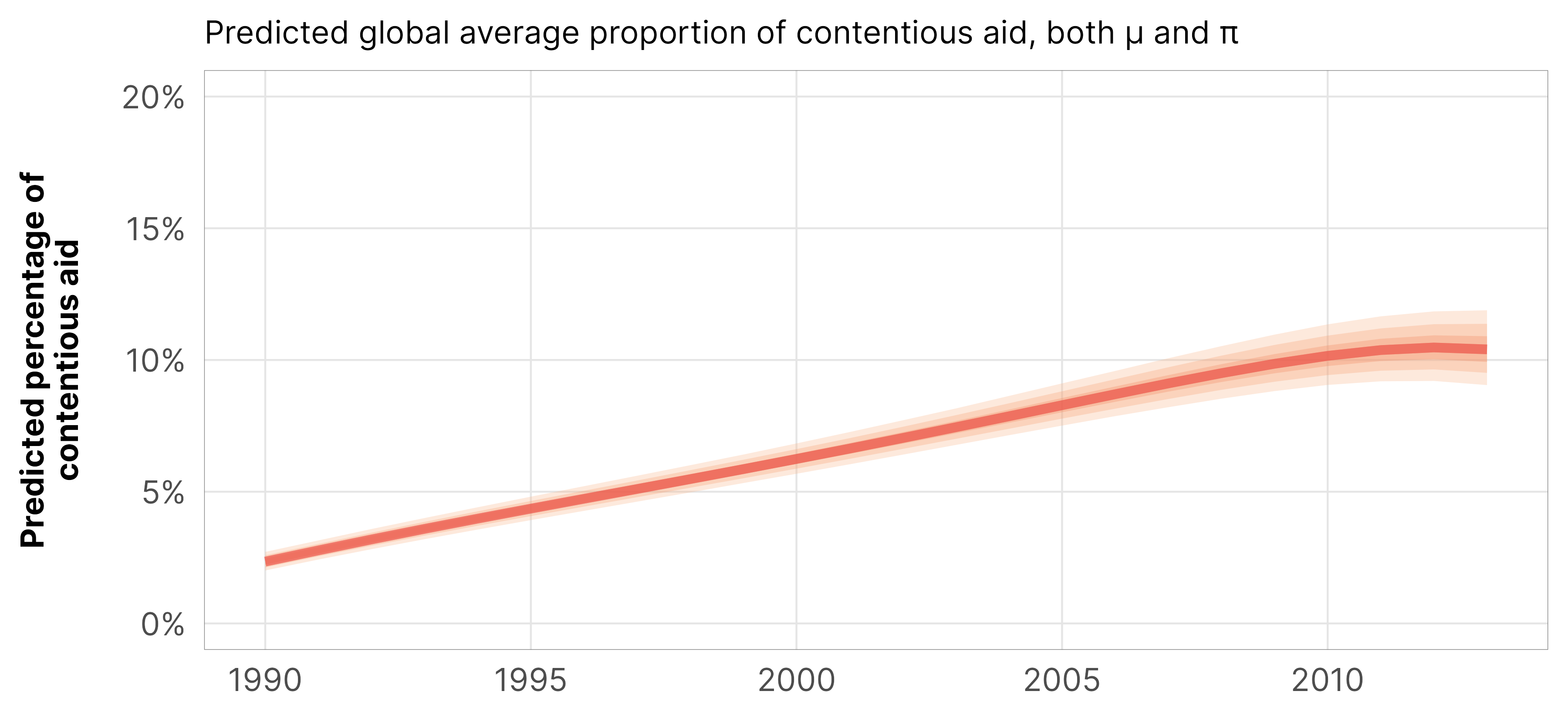
The plot of epred values is different from the linear predictor we found with the $\mu$ part only—that’s because we’re now also incorporating the on/off process. This is actually really pretty neat! The epred values are lower than the linpred values in earlier years, since there’s a higher proportion of 0s in the $\pi$ part of the model then. Similarly, the epred trend flattens out completely after 2010 because the high proportion of 0s from $\pi$ balances out the the year effect in $\mu$. Magical mixture models!

Code

plot_zi_epred <- m_purpose_prelim_time_only_total$model %>% 
  epred_draws(newdata = tibble(year_c = seq(-10, 13, 1)),
              re_formula = NA) %>% 
  mutate(year = year_c + 2000) %>% 
  ggplot(aes(x = year, y = .epred)) +
  stat_lineribbon(color = clrs$Peach[7], alpha = 0.3) +
  scale_y_continuous(labels = label_percent()) +
  scale_fill_manual(values = clrs$Peach[3:5]) +
  coord_cartesian(ylim = c(0, 0.20)) +
  guides(fill = "none") +
  labs(x = NULL, y = "Predicted percentage of\ncontentious aid",
       subtitle = "Predicted global average proportion of contentious aid, both µ and π") +
  theme_donors()
plot_zi_epred

Here’s what all three of these plots look like at the same time—just the $\pi$ zero-inflated is-the-system-on-or-off part, just the $\mu$ when-the-system-is-on part, and the combined epred part:

Code

(plot_zi_zi / plot_zi_mu_linpred / plot_zi_epred) +
  plot_annotation(title = "Conditional effect of time on proportion of contentious aid",
                  subtitle = "prop_contentious ~ year + (1 + year | country)\nzi ~ year + I(year^2)",
                  theme = theme(plot.title = element_text(family = "Inter", face = "bold"),
                                plot.subtitle = element_text(family = "Inconsolata")))

Global analysis (βs)

We just looked at the intercept and year effect above, but as with the hurdle models, these are technically incorrect because we used a multilevel model and haven’t dealt with the $b_{0_j}$ $b_{1_j}$ offsets in the intercept and slope.

Instead, we need to look at a specific flavor of statistical effect or estimand—one of these:

Conditional effect = average country: All $b_n$ offsets are set to 0 so that the effects or coefficients represent the effect in a typical country with the global average level of a variable.
Marginal effect = countries on average: All $b_n$ offsets are dealt with mathematically (averaged/marginalized out or integrated out) so that the effects or coefficients represent the effect of a variable across all countries on average.

Again, we’re generally more interested in conditional effects, but we’ll look at both here just for reference.

Conditional effects

The effect we care about here is the instantaneous slope/partial derivative of year. Rather than figure out the formal calculus for that, we’ll use marginaleffects() to calculate the numerical derivative, which finds the predicted value of $Y$ at some value of $X$, finds the predicted value of $Y$ at some value of $X$ plus a tiny bit ($\varepsilon$ here), subtracts them, and divides by $\varepsilon$. For our situation here, it looks like this mess:

\[ \frac{\textbf{E}(\text{Proportion}_{i_j} \mid \{b_{0_j}, b_{0_j}\} = 0, \text{Year} = t + \varepsilon) - \textbf{E}(\text{Proportion}_{i_j} \mid \{b_{0_j}, b_{0_j}\} = 0, \text{Year} = t)}{\varepsilon} \]

Again, {brms}’s syntax for $\{b_{0_j}, b_{0_j}\} = 0$ (i.e. setting all the random offsets to zero) is to use re_formula = NA in the different functions that generate predictions.

To see what this estimand looks like, it’s helpful to first look at range of predicted values of the proportion of contentious aid so we can see what line we’re finding the slope for. To help with the intuition we’ll look at the plots on both the link (logid) scale and the back-transformed response (percentage point) scale.

We can do this automatically with marginaleffects::plot_cap():

Code

# Log scale
plot_cap(m_purpose_prelim_time_only_total$model, 
         condition = "year_c", type = "link", 
         re_formula = NA)

# Dollar scale
plot_cap(m_purpose_prelim_time_only_total$model, 
         condition = "year_c", type = "response", 
         re_formula = NA)

Or more manually with epred_draws():

Code

preds_logit_zi <- m_purpose_prelim_time_only_total$model %>% 
  linpred_draws(newdata = tibble(year_c = seq(-10, 13, 1)),
                re_formula = NA) %>% 
  mutate(year = year_c + 2000) %>% 
  ggplot(aes(x = year, y = .linpred)) +
  stat_lineribbon(color = clrs$Peach[7]) +
  scale_fill_manual(values = clrs$Peach[1:3]) +
  guides(fill = "none") +
  labs(x = NULL, y = "Predicted proportion of\ncontentious foreign aid, logit scale") +
  theme_donors()

preds_prop_zi <- m_purpose_prelim_time_only_total$model %>% 
  epred_draws(newdata = tibble(year_c = seq(-10, 13, 1)),
              re_formula = NA) %>% 
  mutate(year = year_c + 2000) %>% 
  ggplot(aes(x = year, y = .epred)) +
  stat_lineribbon(color = clrs$Peach[7]) +
  scale_y_continuous(labels = label_percent()) +
  scale_fill_manual(values = clrs$Peach[1:3]) +
  guides(fill = "none") +
  labs(x = NULL, y = "Predicted proportion of\ncontentious foreign aid") +
  theme_donors()

preds_logit_zi | preds_prop_zi

We can use marginaleffects() to get the exact slope of those lines at any value of year_c that we want, and we can plot those slopes across the whole range of years. On the logit scale, the line is flat, since the slope is constant; on the proportion scale, it is generally flat until right after 2005 when it takes a sharp downturn, representing the flattening of the curve. Note that the logit-scale conditional effect is flat, while the proportion scale effect is all weird and drops off quickly. In theory these two plots should look the same. The difference is because {marginaleffects} uses epred values when you specify type = "response", which means that the proportion-scale conditional effect incorporates the zero-process. When we specify type = "link", we get logit-scale effects, but those don’t incorporate the zero process because {marginaleffects} uses linpred values.

Code

mfx_logit_zi <- marginaleffects(
  m_purpose_prelim_time_only_total$model, 
  newdata = datagrid(year_c = seq(-10, 13, by = 1)),
  variables = "year_c",
  type = "link",
  re_formula = NA
)

mfx_prop_zi <- marginaleffects(
  m_purpose_prelim_time_only_total$model, 
  newdata = datagrid(year_c = seq(-10, 13, by = 1)),
  variables = "year_c",
  type = "response",
  re_formula = NA
)

Code

plot_mfx_logit_zi <- mfx_logit_zi %>% 
  posteriordraws() %>% 
  mutate(year = year_c + 2000) %>% 
  ggplot(aes(x = year, y = exp(draw))) +
  stat_lineribbon(color = clrs$PurpOr[7]) +
  scale_fill_manual(values = clrs$PurpOr[1:3]) +
  guides(fill = "none") +
  labs(x = NULL, y = "Conditional effect (logit)") +
  theme_donors()

plot_mfx_prop_zi <- mfx_prop_zi %>% 
  posteriordraws() %>% 
  mutate(year = year_c + 2000) %>% 
  ggplot(aes(x = year, y = draw)) +
  stat_lineribbon(color = clrs$PurpOr[7]) +
  scale_y_continuous(labels = label_percent()) +
  scale_fill_manual(values = clrs$PurpOr[1:3]) +
  guides(fill = "none") +
  labs(x = NULL, y = "Conditional effect (percentage points)") +
  theme_donors()

plot_mfx_logit_zi | plot_mfx_prop_zi

To help even more with the intuition, here are the exact slopes (or conditional effects) at 1990, 2000, 2010, and 2012, both on the logit scale and the percentage point (pp) scale:

Code

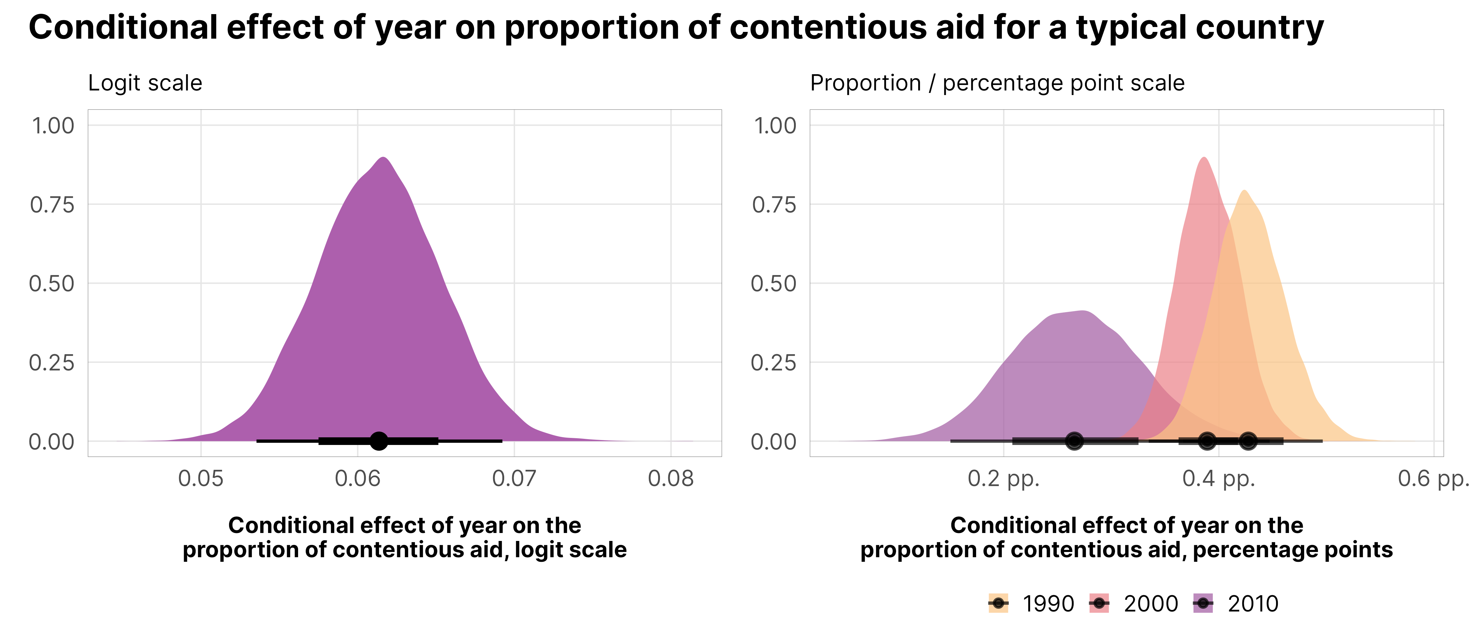
mfx_logit_zi_small <- mfx_logit_zi %>% 
  filter(year_c %in% c(-10, 0, 10, 12)) %>% 
  mutate(year = 2000 + year_c) %>% 
  select(year, dydx, conf.low, conf.high)

mfx_prop_zi_small <- mfx_prop_zi %>% 
  filter(year_c %in% c(-10, 0, 10, 12)) %>% 
  mutate(year = 2000 + year_c) %>% 
  select(year, dydx, conf.low, conf.high) %>% 
  mutate(across(c(dydx, conf.low, conf.high), ~label_number(scale = 100, suffix = " pp.")(.)))

mfx_logit_zi_small
##   year   dydx conf.low conf.high
## 1 1990 0.0614   0.0535    0.0692
## 2 2000 0.0614   0.0535    0.0692
## 3 2010 0.0614   0.0535    0.0692
## 4 2012 0.0614   0.0535    0.0692
mfx_prop_zi_small
##   year      dydx   conf.low conf.high
## 1 1990 0.427 pp.  0.367 pp. 0.497 pp.
## 2 2000 0.389 pp.  0.335 pp. 0.447 pp.
## 3 2010 0.266 pp.  0.150 pp. 0.391 pp.
## 4 2012 0.026 pp. -0.166 pp. 0.211 pp.

Interpretation time. We can look at these effects a few different ways. On the logit scale, a one-year increase in time is associated with a 0.061 increase in the proportion of contentious aid. Exponentiated beta-model effects also don’t make a lot of sense (a increase in the likelihood of some increase in the proportion? idk).

Working with the proportion/percentage point scale is a lot easier—though it varies across time. In 1990 the conditional effect of a one-year increase in time is 0.427 pp. of contentious aid, while in 2000 it is 0.389 pp. and in the flatland of 2012 it is 0.026 pp..

For fun, here are the posteriors of these different conditional effects:

Code

p1 <- mfx_logit_zi %>% 
  posteriordraws() %>% 
  filter(year_c == 0) %>% 
  ggplot(aes(x = draw)) +
  stat_halfeye(fill = clrs$PurpOr[5]) +
  labs(x = "Conditional effect of year on the\nproportion of contentious aid, logit scale", 
       y = NULL, subtitle = "Logit scale", fill = NULL) +
  theme_donors()

p2 <- mfx_prop_zi %>% 
  posteriordraws() %>% 
  filter(year_c %in% c(-10, 0, 10)) %>% 
  mutate(year = year_c + 2000) %>% 
  pivot_longer(draw) %>% 
  ggplot(aes(x = value, fill = factor(year))) +
  stat_halfeye(alpha = 0.7) +
  scale_x_continuous(labels = label_number(scale = 100, suffix = " pp.")) +
  scale_fill_manual(values = clrs$Sunset[c(2, 4, 6)]) +
  labs(x = "Conditional effect of year on the\nproportion of contentious aid, percentage points", 
       y = NULL, subtitle = "Proportion / percentage point scale", fill = NULL) +
  theme_donors()

(p1 | p2) + 
  plot_annotation(title = "Conditional effect of year on proportion of contentious aid for a typical country",
                  theme = theme(plot.title = element_text(family = "Inter", face = "bold")))

Again, these are all conditional effects, which means that they represent the effect of year for a typical country, or a country where all the country-specific offsets are 0.

Marginal effects

\[ \frac{\textbf{E}(\text{Proportion}_{i_j} \mid \text{Year} = t + \varepsilon) - \textbf{E}(\text{Proportion}_{i_j} \mid \text{Year} = t)}{\varepsilon} \]

We can do this with marginaleffects() by setting re_formula = NULL instead of re_formula = NA.

Average / marginalize / integrate across existing random effects

Code

mfx_logit_marginal_zi <- marginaleffects(
  m_purpose_prelim_time_only_total$model, 
  newdata = datagrid(gwcode = unique),
  variables = "year_c",
  type = "link",
  re_formula = NULL
)

Code

mfx_logit_marginal_zi %>% tidy()
##   type   term estimate conf.low conf.high
## 1 link year_c   0.0613   0.0556    0.0668

Integrate out random effects

Code

mfx_logit_marginal_zi_int <- marginaleffects(
  m_purpose_prelim_time_only_total$model, 
  variables = "year_c",
  newdata = datagrid(gwcode = c(-1:-200)),
  re_formula = NULL,
  allow_new_levels = TRUE,
  sample_new_levels = "gaussian",
  type = "link"
)

Code

mfx_logit_marginal_zi_int %>% tidy()
##   type   term estimate conf.low conf.high
## 1 link year_c   0.0614   0.0523    0.0707

Comparing the two

As with the hurdle model, since we have so many countries (142 real ones vs. 200 fake ones), the estimates are basically the same. If we were working with fewer real countries, the estimates from the average / marginalize / integrate across approach would be less accurate.

While the posterior means are the same, the integrating out approach has a little more uncertainty associated with it:

Code

data_marginal_zi <- mfx_logit_marginal_zi %>% 
  posteriordraws() %>% 
  group_by(type, term, drawid) %>% 
  summarize(draw = mean(draw))

data_int_zi <- mfx_logit_marginal_zi_int %>% 
  posteriordraws() %>% 
  group_by(type, term, drawid) %>% 
  summarize(draw = mean(draw))

plot_marginal_zi_mfx_both <- ggplot(mapping = aes(x = draw)) +
  stat_halfeye(data = data_int_zi, aes(fill = "Integrated out")) +
  stat_halfeye(data = data_marginal_zi, aes(fill = "Averaged across"), 
               slab_color = "white", slab_linewidth = 0.5) +
  scale_fill_manual(values = clrs$Peach[c(2, 5)]) +
  # coord_cartesian(xlim = c(1, 1.06)) +
  labs(x = "Marginal effect of year on\nproportion of contentious aid, logit scale", y = NULL,
       fill = "Random effect marginalizing method",
       title = "Marginal marginal effects",
       subtitle = "Effect of year on proportion of contentious aid across all countries on average") +
  theme_donors()
plot_marginal_zi_mfx_both

Country-specific analysis (b offsets and ρ)

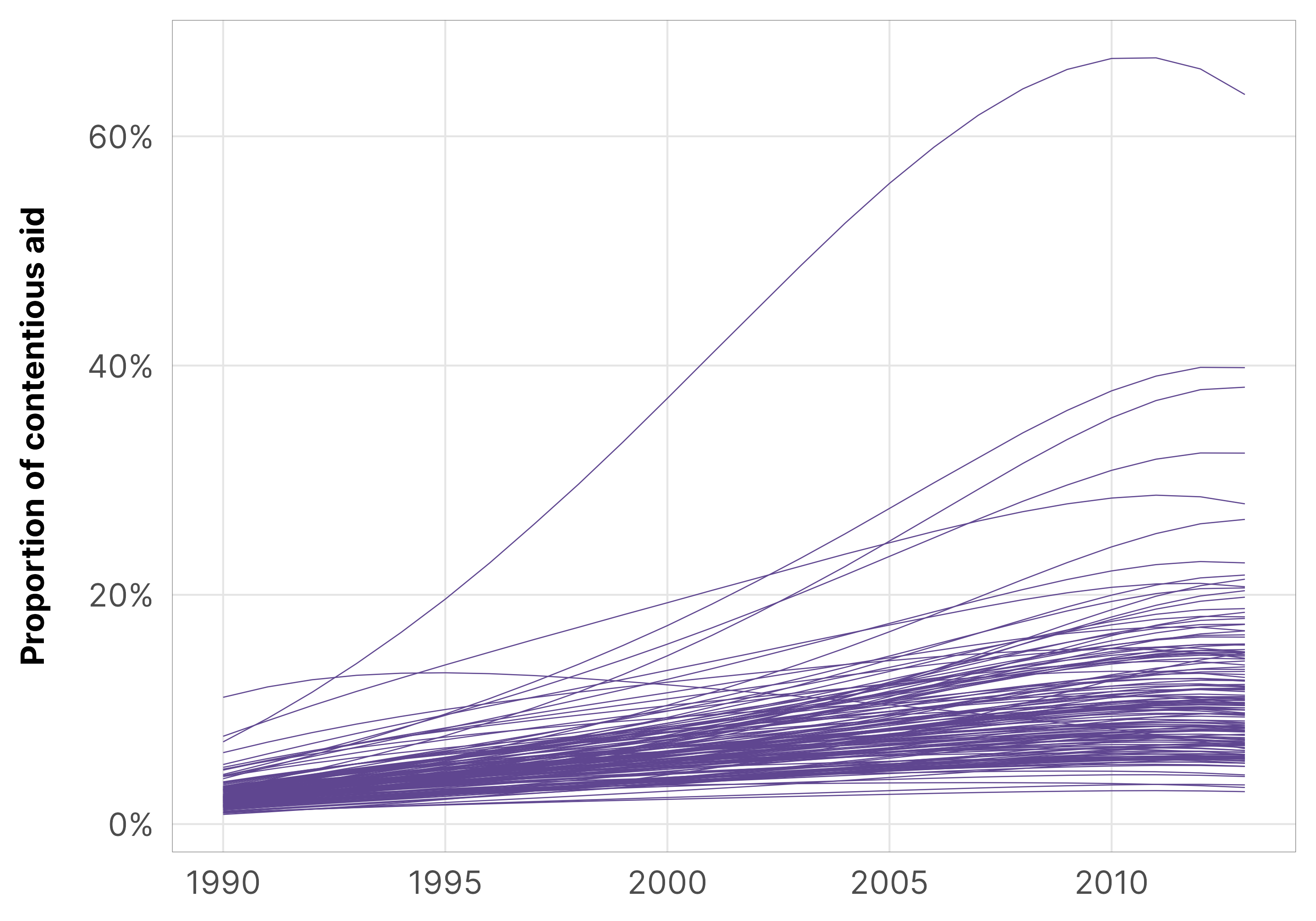
There are 142 different countries, each with their own intercept offsets and slope offsets, so I won’t plot them here. We can look at the first few of these different country-specific offsets to help with the intuition. Each country’s random effects are $b_0$ and $b_1$. These offsets get added to the global averages $\beta_0$ and $\beta_1$, giving each country its own unique slope and intercept.

Code

m_purpose_prelim_time_only_total$model %>%  
  spread_draws(b_Intercept, b_year_c, r_gwcode[gwcode, term]) %>%  
  pivot_wider(names_from = "term", values_from = r_gwcode) %>%  
  mutate(country_intercept = b_Intercept + Intercept,
         country_year_slope = b_year_c + year_c) %>%  
  group_by(gwcode) %>%  
  summarize(across(c(b_Intercept, Intercept, country_intercept, 
                     b_year_c, year_c, country_year_slope), 
                   ~median(.))) %>% 
  rename(`β0` = b_Intercept, `b0 offset` = Intercept, 
         `Intercept` = country_intercept,
         `β1` = b_year_c, `b1 offset` = year_c,
         `Year slope` = country_year_slope)
## # A tibble: 142 × 7
##    gwcode    β0 `b0 offset` Intercept     β1 `b1 offset` `Year slope`
##     <int> <dbl>       <dbl>     <dbl>  <dbl>       <dbl>        <dbl>
##  1     40 -2.62      0.416      -2.20 0.0612    0.0240         0.0852
##  2     41 -2.62      0.755      -1.86 0.0612   -0.0277         0.0336
##  3     42 -2.62     -0.0129     -2.63 0.0612    0.00232        0.0636
##  4     51 -2.62      0.222      -2.40 0.0612    0.0310         0.0923
##  5     52 -2.62     -0.611      -3.23 0.0612    0.0210         0.0823
##  6     70 -2.62     -0.578      -3.20 0.0612    0.00786        0.0692
##  7     90 -2.62      0.853      -1.77 0.0612    0.00105        0.0622
##  8     91 -2.62      0.272      -2.35 0.0612    0.000354       0.0616
##  9     92 -2.62      0.502      -2.12 0.0612   -0.0115         0.0497
## 10     93 -2.62      0.428      -2.19 0.0612   -0.0318         0.0294
## # … with 132 more rows

We can make a spaghetti plot of these country-specific offsets on the percentage point scale:

Code

all_country_lines_zi <- m_purpose_prelim_time_only_total$model %>%  
  epred_draws(expand_grid(gwcode = unique(df_country_aid_laws$gwcode),
                            year_c = seq(-10, 13, by = 1))) %>%  
  group_by(gwcode, year_c) %>%  
  median_qi(.epred) %>%  
  mutate(year = year_c + 2000)

Code

all_country_lines_zi %>% 
  ggplot(aes(x = year, y = .epred)) +
  geom_line(aes(group = gwcode),
            color = clrs$Prism[1], linewidth = 0.15) +
  scale_y_continuous(labels = label_percent()) +
  # scale_y_continuous(trans = log_trans(),
  #                    labels = label_math(e^.x, format = log)) +
  labs(x = NULL, y = "Proportion of contentious aid") +
  theme_donors()

Due to the magic of multilevel models, these intercept and slope offsets are correlated with each other—we modeled the offsets from a multivariate normal distribution, and the correlation between the two $b_{n_j}$ parameters is defined by $\rho_{0, 1}$:

When $\rho$ is negative, bigger intercepts have smaller slopes; when $\rho$ is positive, bigger intercepts have bigger slopes. With our data, if $\rho$ is big and positive it would imply that countries with higher baseline levels of aid contentiousness would see a larger and steeper year effect. In our actual model, $\rho$ is slightly positive, which is neat:

Code

m_purpose_prelim_time_only_total$model %>% 
  spread_draws(cor_gwcode__Intercept__year_c) %>% 
  ggplot(aes(x = cor_gwcode__Intercept__year_c)) +
  stat_halfeye(fill = clrs$Prism[2]) +
  geom_vline(xintercept = 0) +
  labs(x = "ρ<sub>0, 1</sub>", y = NULL) +
  theme_donors() +
  theme(axis.title.x = element_markdown())

Within- and between-country variability (φ and σs)

Finally, we can look at all the terms related to uncertainty. We have three to work with:

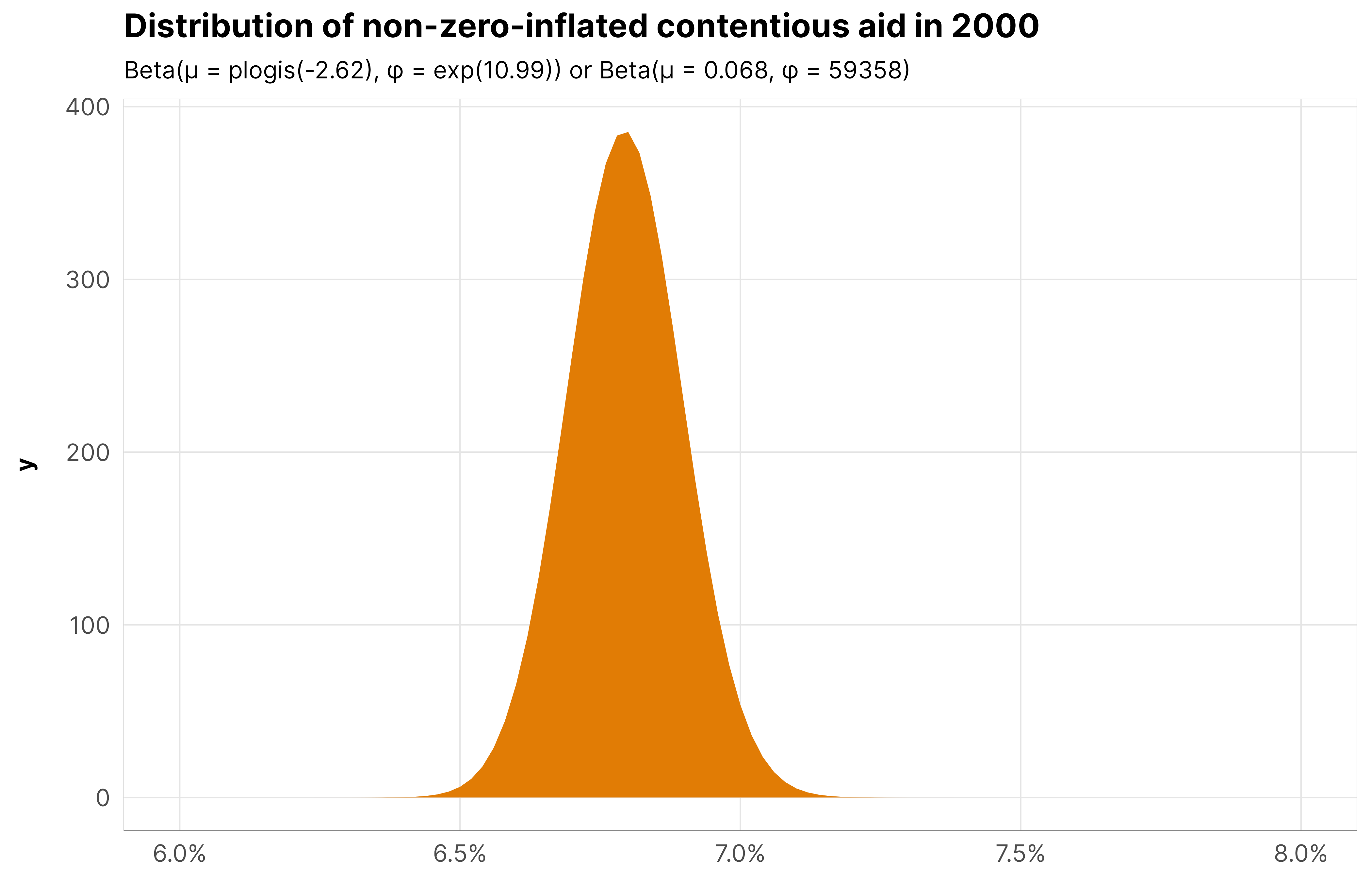
$\phi_y$ (phi): the precision or variance of aid contentiousness within countries. On the log scale, it’s 10.99, which is 59358 when unlogged or exponentiated, which is really really precise. To illustrate this, we can look at the distribution of the proportion of contentious aid when year_c is 0, or in 2000. Based on just a beta distribution with $\mu$ and $\phi$ (i.e. ignoring the zero-inflated part for now), we have a distribution of $\operatorname{Beta}(0.068, 59358)$ which looks like this, very narrowly focused around the baseline average 2000 proportion:

Code

beta_params <- m_purpose_prelim_time_only_total$model %>% 
  tidy(parameters = c("b_(Intercept)", "phi"))

beta_mu <- beta_params %>% 
  filter(term == "b_(Intercept)") %>% 
  pull(estimate)

beta_phi <- beta_params %>% 
  filter(term == "phi") %>% 
  pull(estimate)

ggplot() +
  stat_function(geom = "area", fill = clrs$Prism[7],
                fun = ~dprop(., mean = plogis(beta_mu), size = exp(beta_phi))) +
  scale_x_continuous(labels = label_percent(), limits = c(0.06, 0.08)) +
  labs(title = "Distribution of non-zero-inflated contentious aid in 2000",
       subtitle = glue::glue("Beta(µ = plogis({round(beta_mu, 2)}), φ = exp({round(beta_phi, 2)})) or Beta(µ = {round(plogis(beta_mu), 3)}, φ = {round(exp(beta_phi), 0)})")) +
  theme_donors()

$\sigma_0$ (sd__(Intercept) for the gwcode group): the variability between countries’ baseline averages, or the variability around the $b_{0_j}$ offsets. Here it’s 0.51, which means that across or between countries, the proportion of contentious aid by 0.5 logit units.
$\sigma_1$ (sd__year_c for the gwcode group): the variability between countries’ year effects, or the variability around the $b_{1_j}$ offsets. Here it’s 0.03, which means that average year effects vary by 0.03 logit units across or between countries.

Code

m_purpose_prelim_time_only_total$model %>% 
  tidy(parameters = c("sd_*", "phi")) %>% 
  select(-component)
## # A tibble: 3 × 5
##   term                   estimate std.error conf.low conf.high
##   <chr>                     <dbl>     <dbl>    <dbl>     <dbl>
## 1 sd_gwcode__(Intercept)   0.507    0.0421    0.430     0.596 
## 2 sd_gwcode__year_c        0.0345   0.00506   0.0253    0.0450
## 3 phi                     11.0      0.348    10.3      11.7

Like the hurdle model, we still can’t get an ICC for the percent of variation explained by between-country differences:

Code

performance::icc(m_purpose_prelim_time_only_total$model)
## [1] NA

But we can use performance::variance_decomposition() to get a comparable number, since it uses the posterior predictive distribution of the model to figure out the between-country variance. Between-country differences explain just 36ish% of the variation in the proportion of contentious aid, meaning that within-country differences (or time-based differences) matter a lot more in this case. That’s cool.

Code

performance::variance_decomposition(m_purpose_prelim_time_only_total$model)
## # Random Effect Variances and ICC
## 
## Conditioned on: all random effects
## 
## ## Variance Ratio (comparable to ICC)
## Ratio: 0.36  CI 95%: [0.24 0.47]
## 
## ## Variances of Posterior Predicted Distribution
## Conditioned on fixed effects: 0.01  CI 95%: [0.01 0.01]
## Conditioned on rand. effects: 0.01  CI 95%: [0.01 0.01]
## 
## ## Difference in Variances
## Difference: 0.00  CI 95%: [0.00 0.01]

References

Frees, Edward W. 2009. Regression Modeling with Actuarial and Financial Applications. New York: Cambridge University Press. https://doi.org/10.1017/cbo9780511814372.

Keele, Luke, Randolph T. Stevenson, and Felix Elwert. 2020. “The Causal Interpretation of Estimated Associations in Regression Models.” Political Science Research and Methods 8 (1): 1–13. https://doi.org/10.1017/psrm.2019.31.

McElreath, Richard. 2020. Statistical Rethinking: A Bayesian Course with Examples in R and Stan. 2nd ed. Boca Raton, Florida: Chapman and Hall / CRC.

Muff, Stefanie, Leonhard Held, and Lukas F. Keller. 2016. “Marginal or Conditional Regression Models for Correlated Non-Normal Data?” Methods in Ecology and Evolution 7 (12): 1514–24. https://doi.org/10.1111/2041-210X.12623.

Schielzeth, Holger. 2010. “Simple Means to Improve the Interpretability of Regression Coefficients.” Methods in Ecology and Evolution 1 (2): 103–13. https://doi.org/10.1111/j.2041-210X.2010.00012.x.

Westreich, Daniel, and Sander Greenland. 2013. “The Table 2 Fallacy: Presenting and Interpreting Confounder and Modifier Coefficients.” American Journal of Epidemiology 177 (4): 292–98. https://doi.org/10.1093/aje/kws412.