We identify our time-varying and time-invariant confounders based on our causal model and do-calculus logic, and we deal with the panel structure of the data by including random intercepts for country, and both a population-level trend and random slopes for year. We use generic weakly informative priors for our model parameters.
Numerator
Our numerator models look like this (but with the actual treatment variable replacing treatment, like barriers_total, advocacy, and so on):
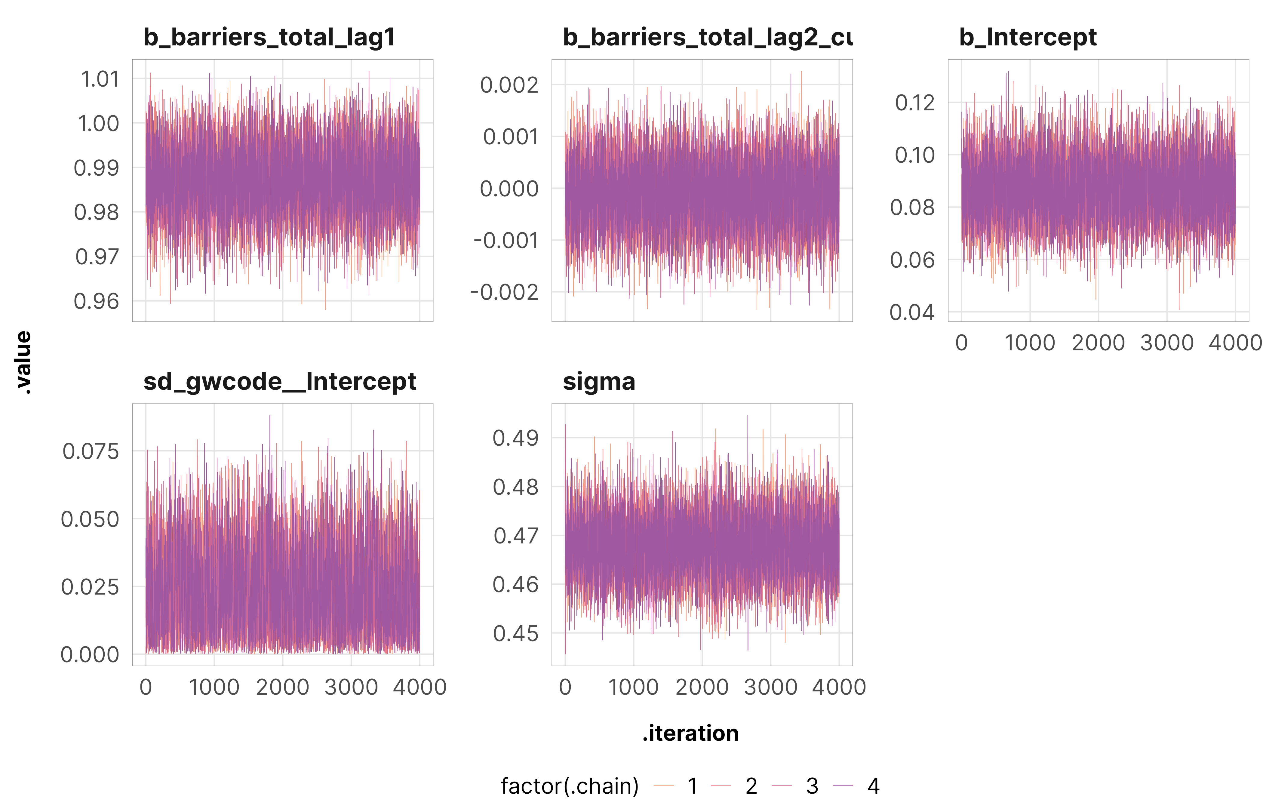
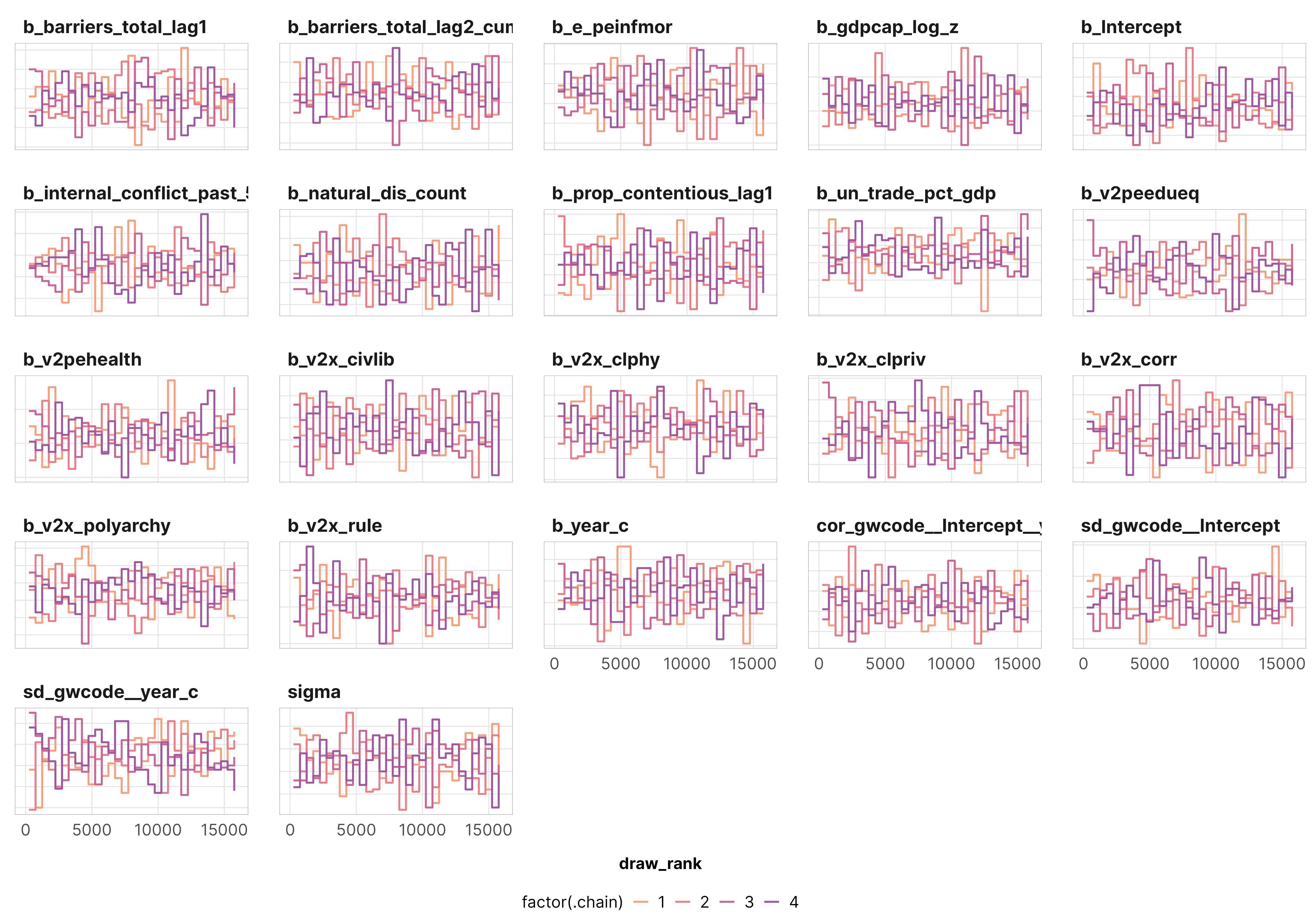
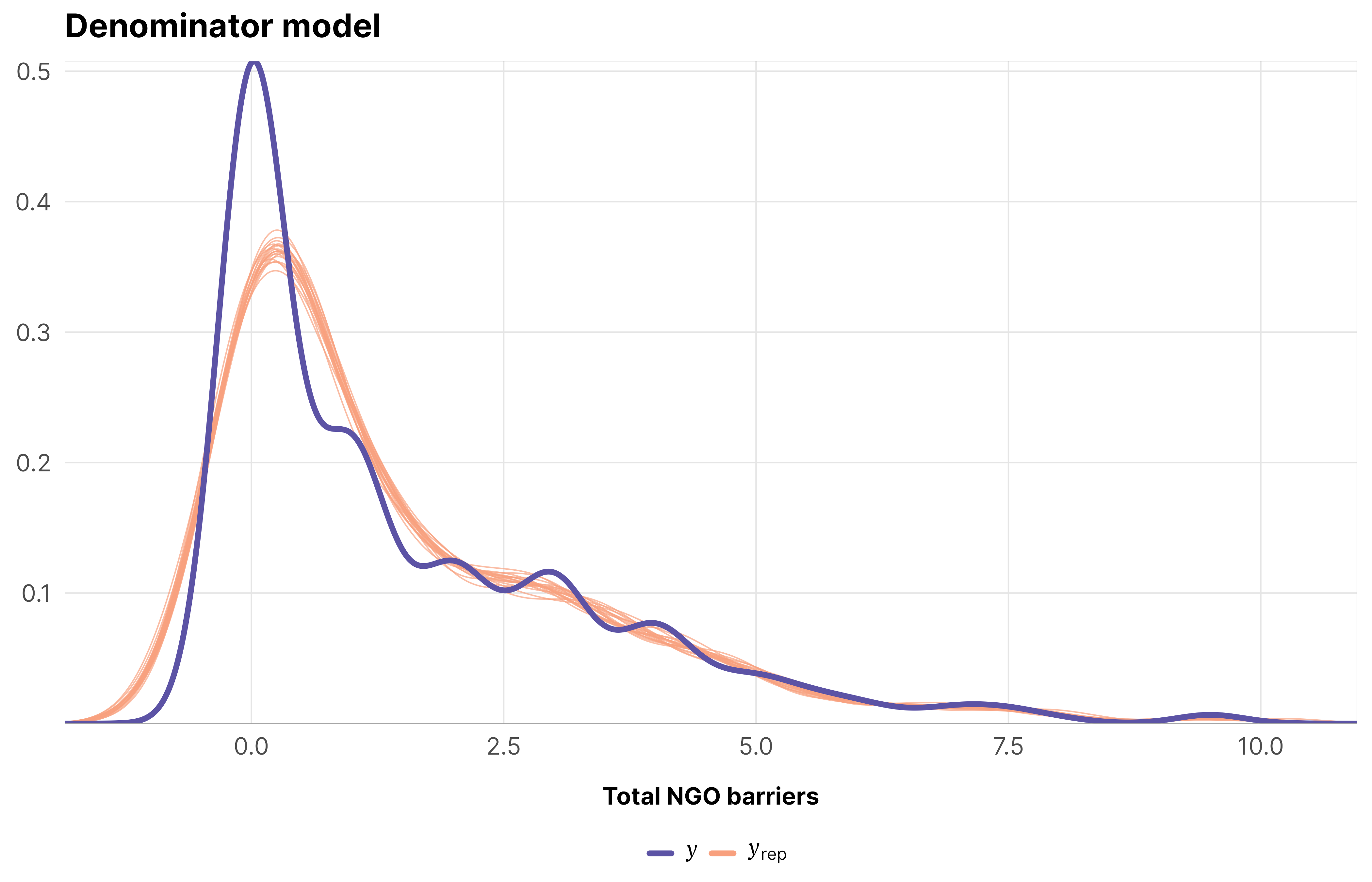
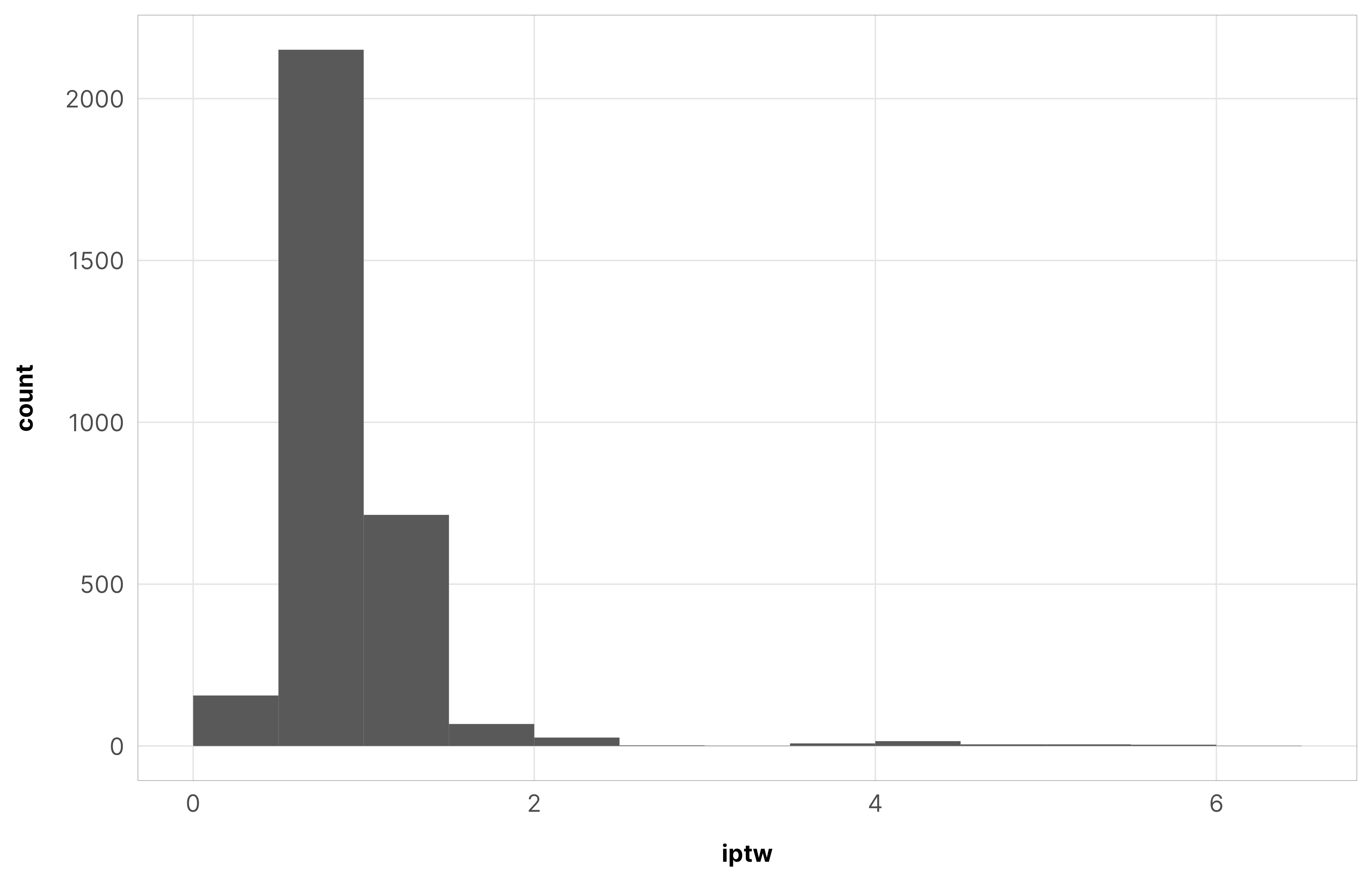
Again, as a check to make sure these weight models converged, here are some visual diagnostics for the total barriers treatment. All the other models look basically the same as these.
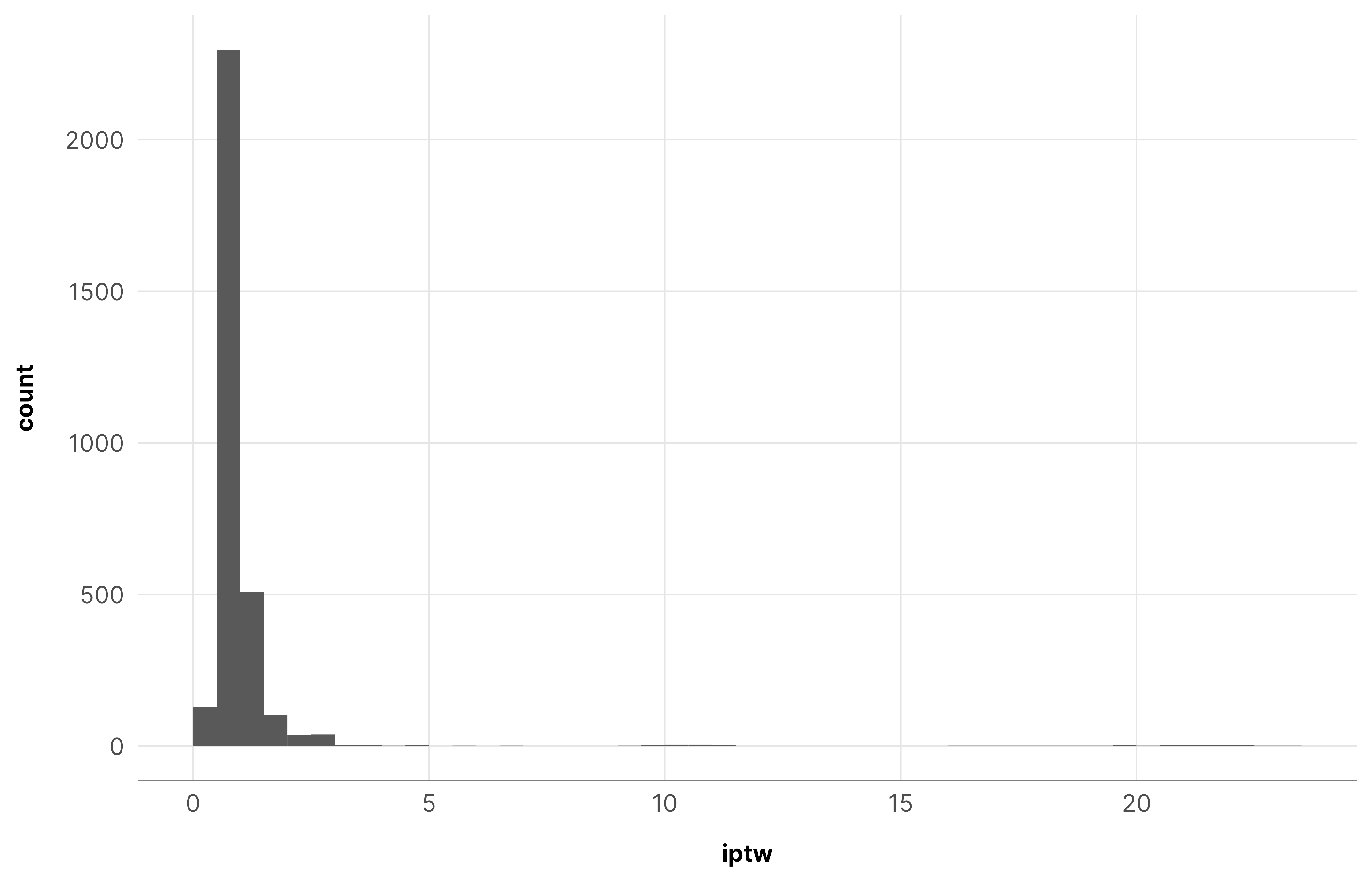
The max weight here is 23, but as with H1 there are only a few observations with weights that high. The average is 1.12 and the median is 0.9, which are both close to 1, which is good.
Code
summary(df_purpose_iptw_total$iptw)## Min. 1st Qu. Median Mean 3rd Qu. Max. ## 0.05 0.78 0.90 1.12 1.00 23.34
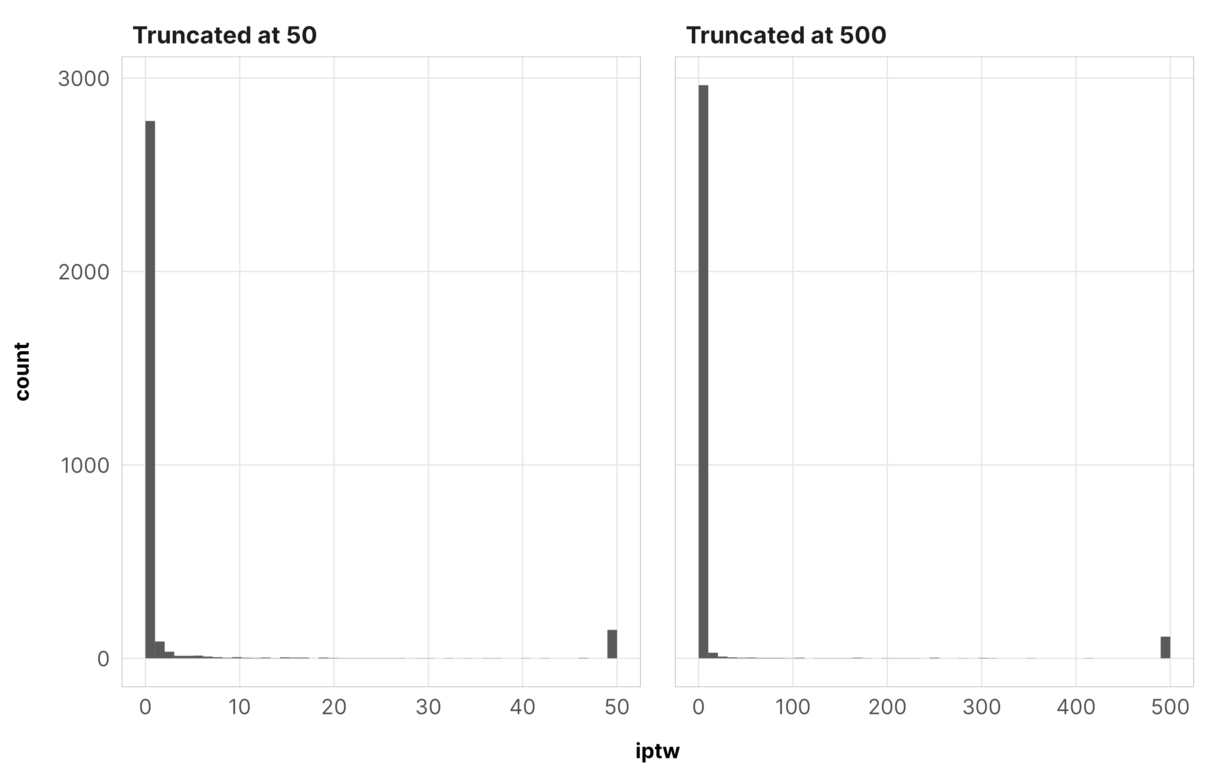
So we truncate these weights at 50 again. Since the results from the core civil society models are basically the same when truncating at 500, we only use a truncation point of 50 here.
These are less important since we just use these treatment models to generate weights and because interpreting each coefficient when trying to isolate causal effects is unimportant (Westreich and Greenland 2013; Keele, Stevenson, and Elwert 2020).
models_tbl_h2_treatment_num <- models_tbl_h2_treatment_num %>%set_names(1:length(.))notes <-c("Posterior medians; 95% credible intervals in brackets", "Total \\(R^2\\) considers the variance of both population and group effects", "Marginal \\(R^2\\) only takes population effects into account")modelsummary(models_tbl_h2_treatment_num,estimate ="{estimate}",statistic ="[{conf.low}, {conf.high}]",add_rows = treatment_rows,coef_map = coefs_num,gof_map = gofs,output ="kableExtra",fmt =list(estimate =2, conf.low =2, conf.high =2)) %>%row_spec(1, bold =TRUE) %>%kable_styling(htmltable_class ="table-sm light-border")
Table 1: Results from all numerator models
1
2
3
4
5
6
Treatment
Total barriers (t)
Barriers to advocacy (t)
Barriers to entry (t)
Barriers to funding (t)
CCSI (t)
CS repression (t)
Treatment (t − 1)
0.99
1.00
0.97
0.99
0.82
0.84
[0.97, 1.00]
[0.98, 1.01]
[0.96, 0.99]
[0.97, 1.00]
[0.80, 0.84]
[0.82, 0.86]
Treatment history
−0.0001
−0.0005
−0.0003
0.0002
−0.0007
−0.002
[−0.001, 0.001]
[−0.002, 0.0007]
[−0.002, 0.0009]
[−0.001, 0.002]
[−0.001, −0.0002]
[−0.004, −0.001]
Intercept
0.09
0.02
0.05
0.03
0.13
0.13
[0.07, 0.11]
[0.01, 0.02]
[0.04, 0.07]
[0.02, 0.04]
[0.11, 0.14]
[0.08, 0.17]
Between-country variability (\(\sigma_0\) for \(b_0\) offsets)
0.02
0.005
0.01
0.009
0.05
0.25
[0.001, 0.06]
[0.0002, 0.01]
[0.0008, 0.04]
[0.0004, 0.03]
[0.04, 0.06]
[0.21, 0.30]
Model variability (\(\sigma_y\))
0.47
0.12
0.24
0.23
0.06
0.31
[0.46, 0.48]
[0.12, 0.12]
[0.24, 0.25]
[0.22, 0.23]
[0.05, 0.06]
[0.30, 0.32]
N
3011
3011
3011
3011
3130
3272
\(R^2\) (total)
0.94
0.95
0.92
0.94
0.96
0.95
\(R^2\) (marginal)
0.94
0.95
0.92
0.94
0.90
0.89
Code
models_tbl_h2_treatment_denom <- models_tbl_h2_treatment_denom %>%set_names(1:length(.))notes <-c("Posterior medians; 95% credible intervals in brackets", "Total \\(R^2\\) considers the variance of both population and group effects", "Marginal \\(R^2\\) only takes population effects into account")modelsummary(models_tbl_h2_treatment_denom,estimate ="{estimate}",statistic ="[{conf.low}, {conf.high}]",add_rows = treatment_rows,coef_map = coefs_denom,gof_map = gofs,fmt =list(estimate =2, conf.low =2, conf.high =2),notes = notes) %>%row_spec(1, bold =TRUE) %>%kable_styling(htmltable_class ="table-sm light-border")
Table 2: Results from all numerator models
1
2
3
4
5
6
Treatment
Total barriers (t)
Barriers to advocacy (t)
Barriers to entry (t)
Barriers to funding (t)
CCSI (t)
CS repression (t)
Treatment (t − 1)
0.97
0.98
0.97
0.97
0.33
0.45
[0.96, 0.99]
[0.96, 1.00]
[0.95, 0.98]
[0.95, 0.99]
[0.30, 0.36]
[0.42, 0.48]
Treatment history
−0.0008
0.0002
−0.001
0.00007
−0.002
−0.003
[−0.002, 0.0007]
[−0.002, 0.002]
[−0.002, 0.0004]
[−0.001, 0.002]
[−0.003, 0.0001]
[−0.005, −0.001]
Proportion of contentious aid (t − 1)
−0.005
0.01
0.002
−0.008
−0.001
0.05
[−0.18, 0.17]
[−0.03, 0.06]
[−0.09, 0.09]
[−0.09, 0.08]
[−0.02, 0.02]
[−0.05, 0.16]
Polyarchy
−0.12
0.02
−0.10
−0.05
0.03
−0.03
[−0.29, 0.06]
[−0.02, 0.07]
[−0.19, 0.0002]
[−0.14, 0.04]
[−0.002, 0.06]
[−0.21, 0.15]
Corruption index
−0.11
−0.02
−0.04
−0.05
−0.04
−0.24
[−0.29, 0.06]
[−0.07, 0.03]
[−0.13, 0.06]
[−0.14, 0.04]
[−0.08, 0.007]
[−0.50, 0.01]
Rule of law index
−0.14
−0.04
−0.04
−0.05
0.02
0.22
[−0.34, 0.06]
[−0.09, 0.02]
[−0.14, 0.07]
[−0.15, 0.05]
[−0.03, 0.07]
[−0.06, 0.51]
Civil liberties index
−0.45
−0.16
−0.16
−0.12
0.90
2.92
[−0.98, 0.07]
[−0.30, −0.01]
[−0.44, 0.12]
[−0.38, 0.13]
[0.83, 0.98]
[2.47, 3.36]
Physical violence index
0.26
0.07
0.10
0.07
−0.20
−0.14
[0.03, 0.50]
[0.008, 0.14]
[−0.02, 0.23]
[−0.04, 0.19]
[−0.24, −0.16]
[−0.37, 0.09]
Private civil liberties index
0.15
0.06
0.08
0.004
−0.10
−0.18
[−0.13, 0.43]
[−0.01, 0.14]
[−0.07, 0.23]
[−0.14, 0.14]
[−0.15, −0.06]
[−0.46, 0.10]
Log GDP/capita (standardized)
−0.02
−0.004
−0.005
−0.01
−0.02
−0.02
[−0.05, 0.008]
[−0.01, 0.004]
[−0.02, 0.01]
[−0.03, 0.003]
[−0.03, −0.005]
[−0.09, 0.04]
Percent of GDP from trade
−0.02
0.003
−0.02
−0.01
−0.007
−0.01
[−0.07, 0.02]
[−0.008, 0.02]
[−0.04, 0.006]
[−0.03, 0.01]
[−0.02, 0.002]
[−0.07, 0.04]
Educational equality index
−0.01
−0.0007
−0.002
−0.01
−0.009
0.04
[−0.04, 0.01]
[−0.008, 0.007]
[−0.02, 0.01]
[−0.03, 0.002]
[−0.02, −0.001]
[−0.006, 0.08]
Health equality index
0.02
0.002
0.001
0.02
−0.002
−0.03
[−0.01, 0.05]
[−0.007, 0.01]
[−0.02, 0.02]
[0.002, 0.03]
[−0.01, 0.006]
[−0.07, 0.02]
Infant mortality rate
−0.0006
−0.00005
−0.0001
−0.0004
0.0001
0.0009
[−0.001, 0.0003]
[−0.0003, 0.0002]
[−0.0006, 0.0004]
[−0.0008, 0.00008]
[−0.0002, 0.0004]
[−0.0008, 0.003]
Internal conflict in past 5 years
0.01
0.004
0.005
0.006
0.01
−0.008
[−0.03, 0.06]
[−0.008, 0.02]
[−0.02, 0.03]
[−0.01, 0.03]
[0.005, 0.02]
[−0.05, 0.03]
Count of natural disasters
0.005
0.001
0.002
0.002
0.0001
0.007
[−0.0003, 0.01]
[−0.0004, 0.002]
[−0.0008, 0.005]
[−0.0008, 0.004]
[−0.0007, 0.001]
[0.002, 0.01]
Intercept
0.35
0.04
0.14
0.16
0.05
−1.23
[0.18, 0.52]
[−0.004, 0.09]
[0.05, 0.23]
[0.08, 0.24]
[0.006, 0.10]
[−1.48, −0.98]
Year trend
0.006
0.001
0.003
0.002
0.001
−0.003
[0.003, 0.01]
[−0.00005, 0.002]
[0.001, 0.005]
[0.0008, 0.004]
[−0.00002, 0.003]
[−0.007, 0.002]
Between-country intercept variability (\(\sigma_0\) for \(b_0\) offsets)
0.02
0.009
0.01
0.01
0.06
0.32
[0.0007, 0.05]
[0.001, 0.02]
[0.0006, 0.03]
[0.0005, 0.03]
[0.05, 0.07]
[0.28, 0.38]
Between-country year variability (\(\sigma_{17}\) for \(b_{17}\) offsets)
0.003
0.003
0.001
0.001
0.004
0.02
[0.0001, 0.008]
[0.002, 0.004]
[0.00005, 0.003]
[0.00005, 0.003]
[0.003, 0.004]
[0.02, 0.02]
Correlation between random intercepts and slopes (\(\rho\))
0.06
0.66
0.06
0.02
−0.13
−0.15
[−0.79, 0.82]
[−0.09, 0.95]
[−0.79, 0.82]
[−0.81, 0.82]
[−0.31, 0.06]
[−0.33, 0.05]
Model variability (\(\sigma_y\))
0.46
0.12
0.24
0.22
0.04
0.25
[0.45, 0.48]
[0.12, 0.12]
[0.24, 0.25]
[0.22, 0.23]
[0.04, 0.04]
[0.25, 0.26]
N
3011
3011
3011
3011
3130
3272
\(R^2\) (total)
0.94
0.95
0.93
0.94
0.98
0.97
\(R^2\) (marginal)
0.94
0.95
0.92
0.94
0.92
0.89
Posterior medians; 95% credible intervals in brackets
Total \(R^2\) considers the variance of both population and group effects
Marginal \(R^2\) only takes population effects into account
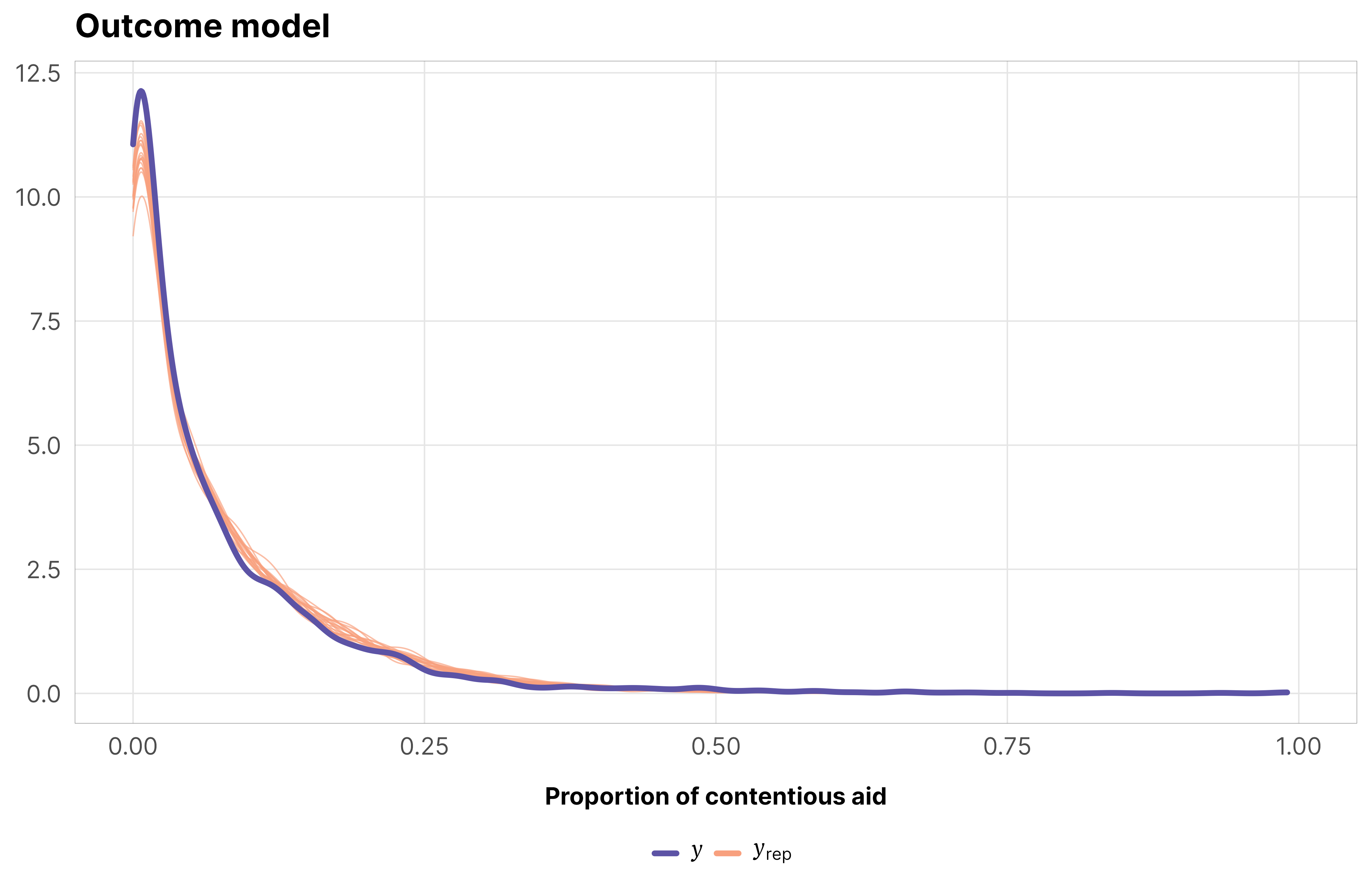
Outcome models
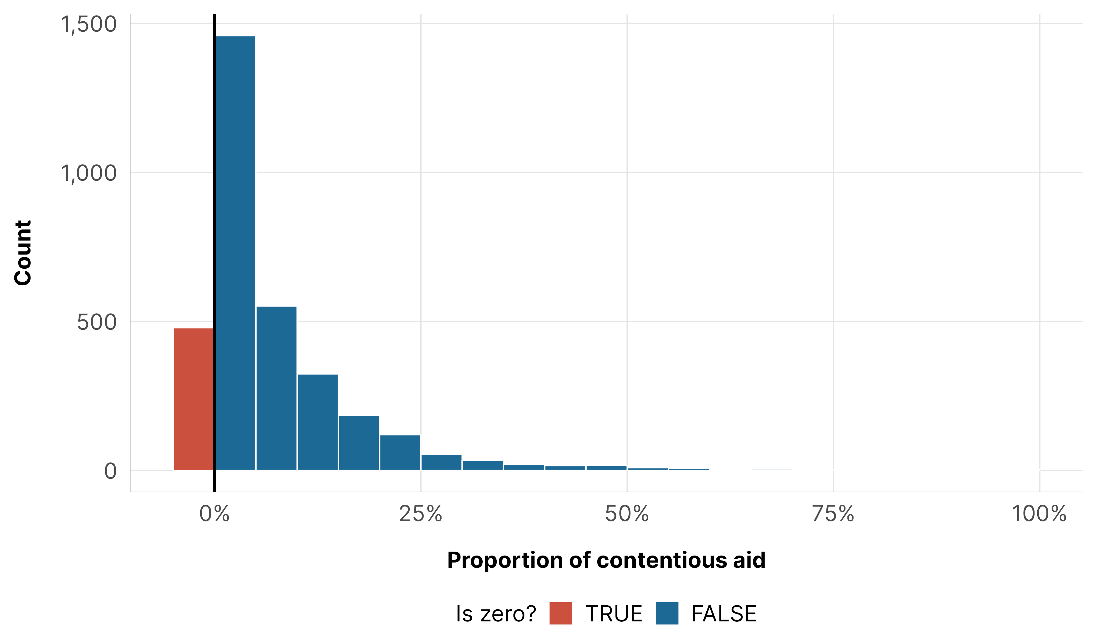
Our outcome variable for this hypothesis is the proportion of aid allocated to contentious issues, which is (1) bounded between 0% and 100% and (2) has a lot of zeros.
Because of this distribution, we use a zero-inflated beta family to model the outcome. This guide to working with tricky outcomes with lots of zeros explores all the intricacies of zero-inflated beta families, so we won’t go into tons of detail here.
Following our marginal structural model approach, we need to run a model weighted by the stabilized inverse probability weights that includes covariates for lagged treatment \(X_{i, t-1}\), treatment history \(\sum_{\tau = (t-2)}^{t} X_{i\tau}\), and non-time-varying confounders \(Z_i\). We expand on this approach to account for the panel structure of the data by using a multilevel hierarchical model with country-specific intercepts and a year trend with country-specific offsets (following yet another guide I wrote for this project, this one on multilevel panel data). We center the year at 2000 so that (1) the intercept is interpretable (Schielzeth 2010) and (2) the MCMC simulation runs faster and more efficiently (McElreath 2020, sec. 13.4, pp. 420–422).
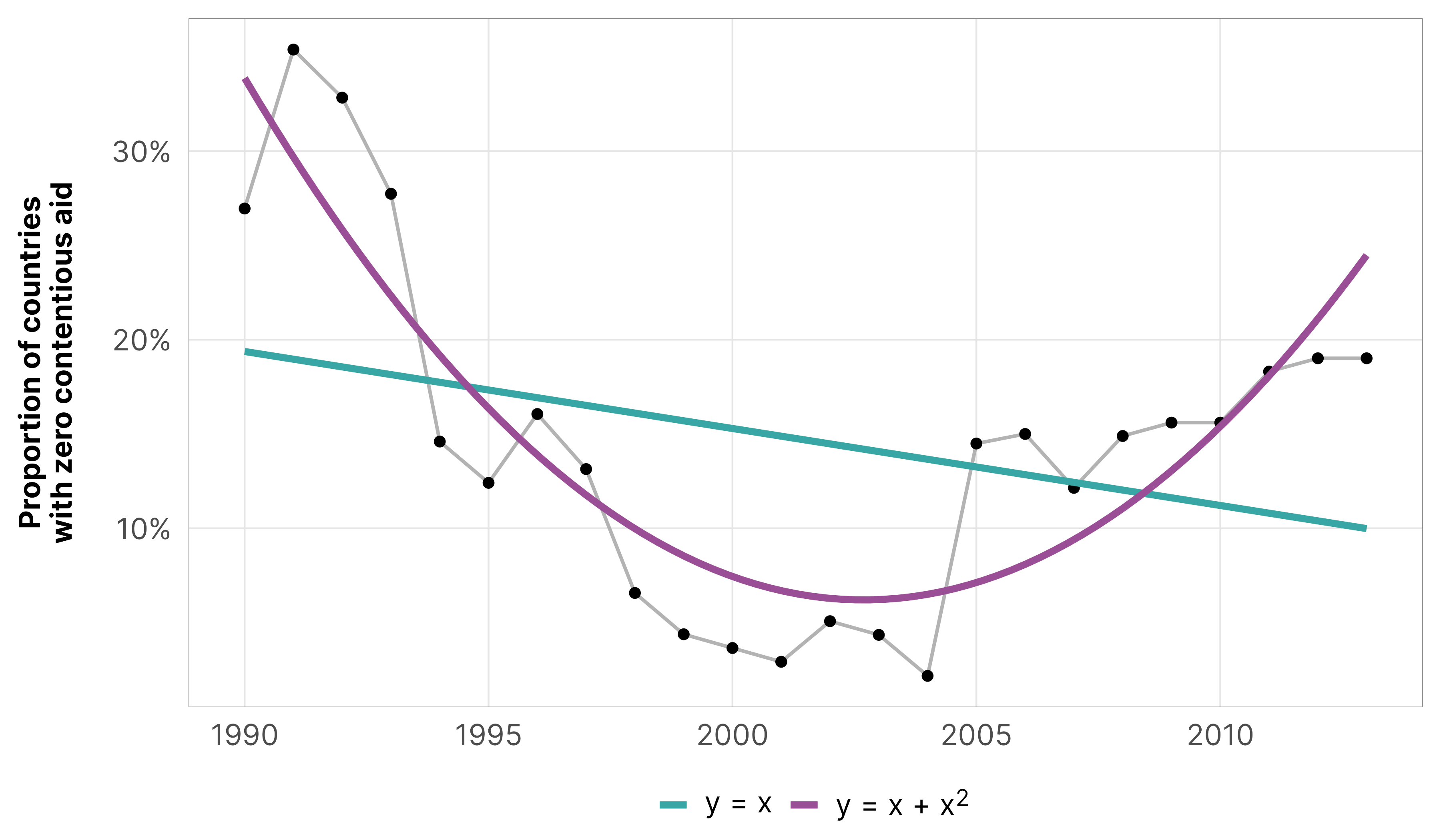
As with foreign aid, we’re not entirely sure what the actual underlying zero process is for the proportion of contentious aid, but from looking at the data, we know that there’s a time component—in the early 2000s, very few countries received no contentious aid. We thus model the zero-inflated part of the model with year and year squared since the year trend is parabolic and nonlinear.
Code
df_country_aid_laws %>%group_by(year) %>%summarize(prop_zero =mean(prop_contentious ==0)) %>%ggplot(aes(x = year, y = prop_zero)) +geom_line(linewidth =0.5, color ="grey70") +geom_point(size =1) +geom_smooth(aes(color ="y = x"), method ="lm", formula = y ~ x, se =FALSE) +geom_smooth(aes(color ="y = x + x<sup>2</sup>"), method ="lm", formula = y ~ x +I(x^2), se =FALSE) +scale_y_continuous(labels =label_percent()) +scale_color_manual(values = clrs$Prism[c(3, 11)]) +labs(x =NULL, y ="Proportion of countries\nwith zero contentious aid",color =NULL) +theme_donors() +theme(legend.text =element_markdown())
Formal model and priors
Our final model looks like this (again with treatment replaced by the actual treatment column):
\[
\begin{aligned}
&\ \mathrlap{\textbf{Zero-inflated model of proportion $i$ across time $t$ within each country $j$}} \\
\text{Proportion}_{it_j} \sim&\ \mathrlap{\begin{cases}
0 & \text{with probability } \pi_{it} + [(1 - \pi_{it}) \times \operatorname{Beta}(0 \mid \mu_{it_j}, \phi_y)] \\[4pt]
\operatorname{Beta}(\mu_{it_j}, \phi_y) & \text{with probability } (1 - \pi_{it}) \times \operatorname{Beta}(\text{Proportion}_{it_j} \mid \mu_{it_j}, \phi_y)
\end{cases}} \\
\\
&\ \textbf{Models for distribution parameters} \\
\operatorname{logit}(\pi_{it}) =&\ \gamma_0 + \gamma_1 \text{Year}_{it} + \gamma_2 \text{Year}^2_{it} & \text{Zero-inflation process} \\[4pt]
\operatorname{logit}(\mu_{it_j}) =&\ \text{IPTW}_{i, t-1_j} \times \Bigl[ (\beta_0 + b_{0_j}) + \beta_1\, \text{Treatment}_{i, t-1_j} + \\
&\ \beta_2\, \textstyle{\sum_{\tau = (t-2)}^{t}} \text{Treatment}_{i\tau} + (\beta_3 + b_{3_j}) \text{Year}_{it_j} \Bigr] & \text{Within-country variation} \\[4pt]
\left(
\begin{array}{c}
b_{0_j} \\
b_{3_j}
\end{array}
\right)
\sim&\ \text{MV}\,\mathcal{N}
\left[
\left(
\begin{array}{c}
0 \\
0 \\
\end{array}
\right)
, \,
\left(
\begin{array}{cc}
\sigma^2_{0} & \rho_{0, 3}\, \sigma_{0} \sigma_{3} \\
\cdots & \sigma^2_{3}
\end{array}
\right)
\right] & \text{Variability in average intercepts and slopes} \\
\\
&\ \textbf{Priors} \\
\gamma_0 \sim&\ \text{Student $t$}(\nu = 3, \mu = 0, \sigma = 1.5) & \text{Prior for intercept in zero-inflated model} \\
\gamma_1, \gamma_2 \sim&\ \text{Student $t$}(3, 0, 1.5) & \text{Prior for year effect in zero-inflated model} \\
\beta_0 \sim&\ \text{Student $t$}(3, 0, 1.5) & \text{Prior for global average proportion} \\
\beta_1, \beta_2, \beta_3 \sim&\ \text{Student $t$}(3, 0, 1.5) & \text{Prior for global effects} \\
\phi_y \sim&\ \operatorname{Exponential}(1) & \text{Prior for within-country dispersion} \\
\sigma_0, \sigma_3 \sim&\ \operatorname{Exponential}(1) & \text{Prior for within-country variability} \\
\rho \sim&\ \operatorname{LKJ}(2) & \text{Prior for between-country variability}
\end{aligned}
\]
Here’s what those priors look like:
Code
design <-" AAABBB CCCDDD EEFFGG"m_purpose_outcome_total$priors %>%parse_dist() %>%# K = dimension of correlation matrix; # ours is 2x2 here because we have one random slopemarginalize_lkjcorr(K =2) %>%mutate(nice_title =glue("**{class}**: {prior}"),stage =ifelse(dpar =="zi", "Zero-inflated part (π)", "Beta part (µ and φ)")) %>%mutate(nice_title =fct_inorder(nice_title),stage =fct_rev(fct_inorder(stage))) %>%ggplot(aes(y =0, dist = .dist, args = .args, fill = prior)) +stat_slab(normalize ="panels") +scale_fill_manual(values = clrs$Prism[1:6]) +facet_manual(vars(stage, nice_title), design = design, scales ="free_x",strip =strip_nested(background_x =list(element_rect(fill ="grey92"), NULL),by_layer_x =TRUE)) +guides(fill ="none") +labs(x =NULL, y =NULL) +theme_donors(prior =TRUE) +theme(strip.text =element_markdown())
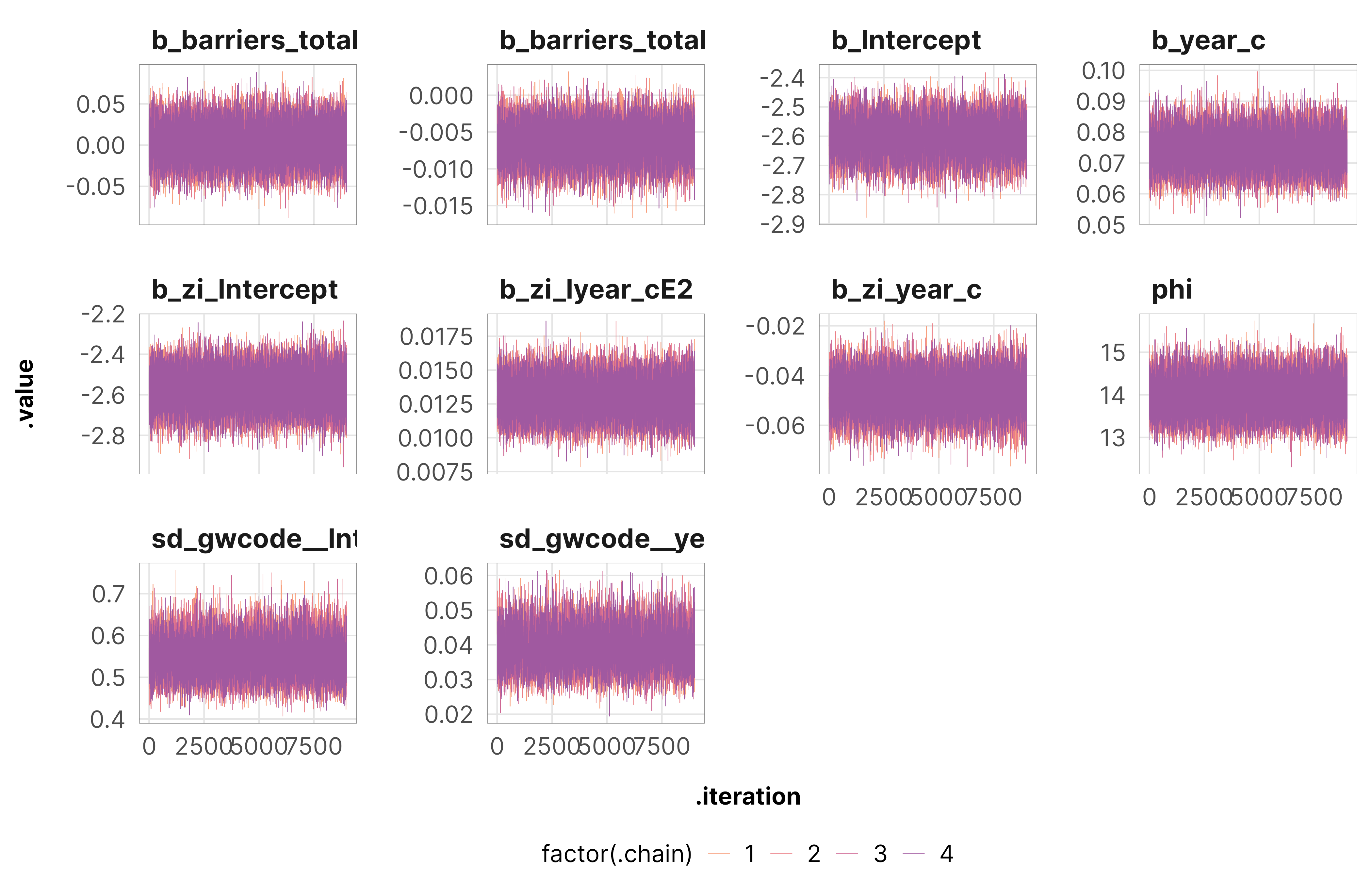
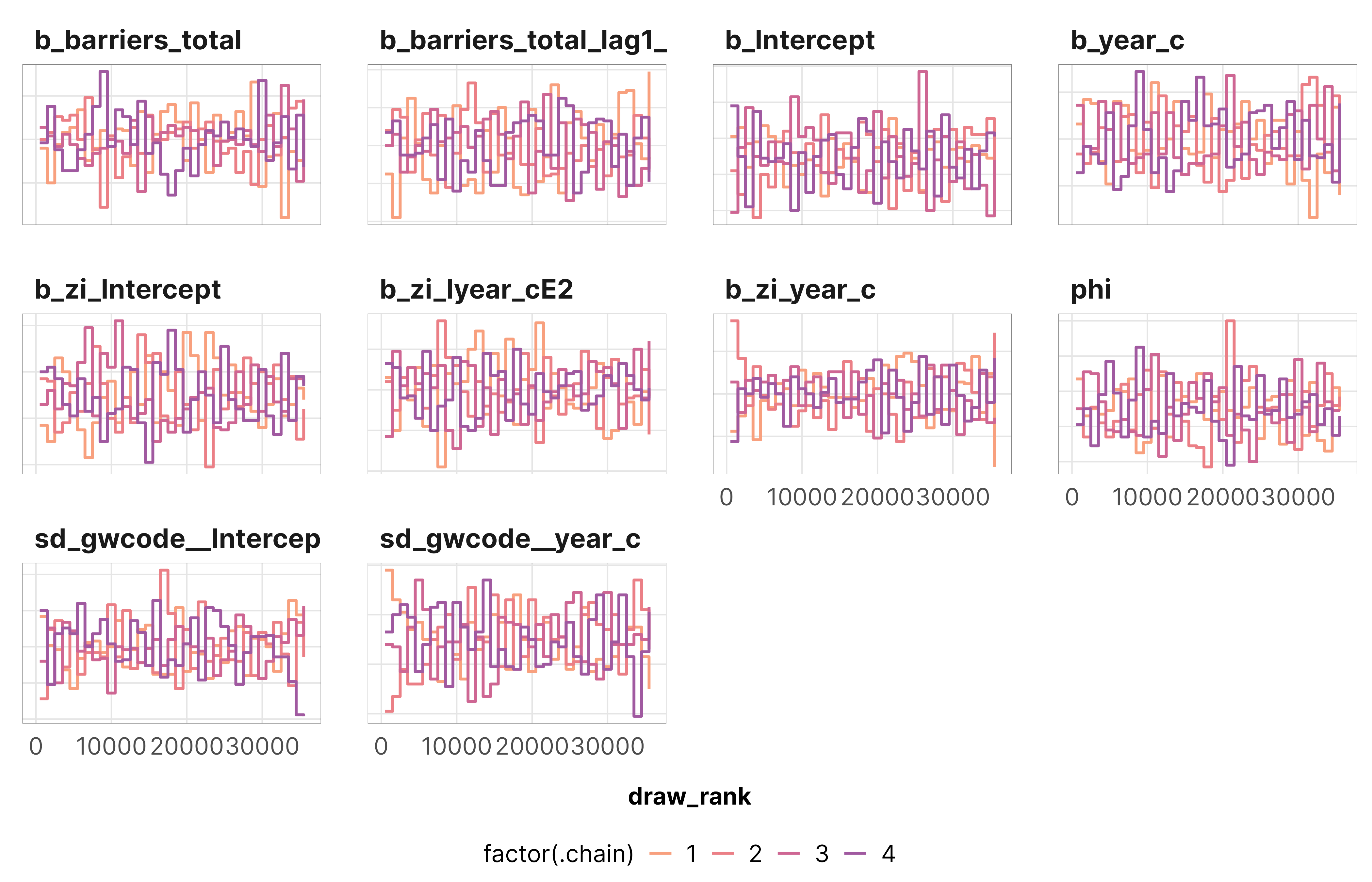
MCMC diagnostics
To check that everything converged nicely, we check some diagnostics for the outcome models for the total barriers treatment. All the other models look basically the same as this—everything’s fine.
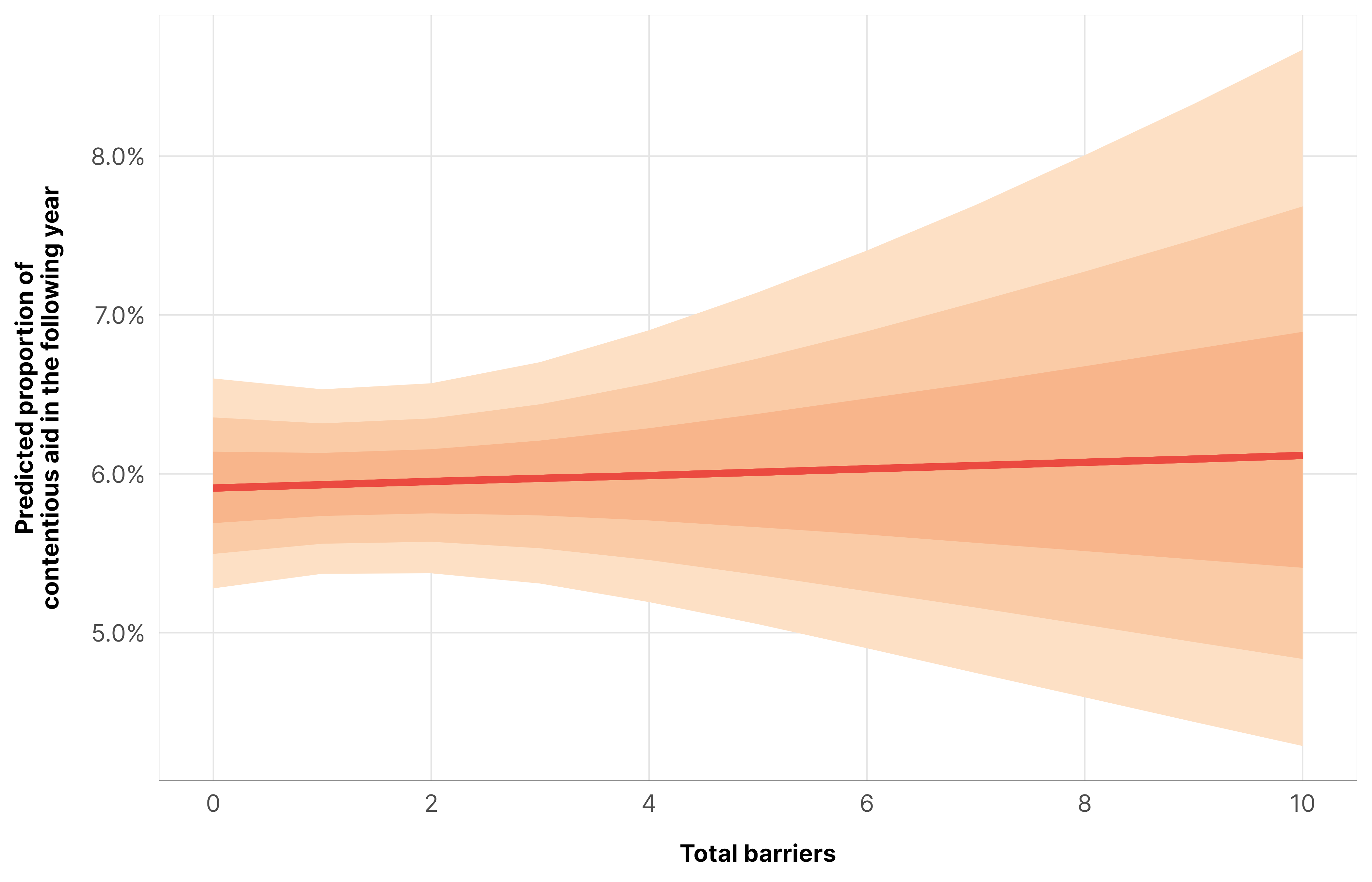
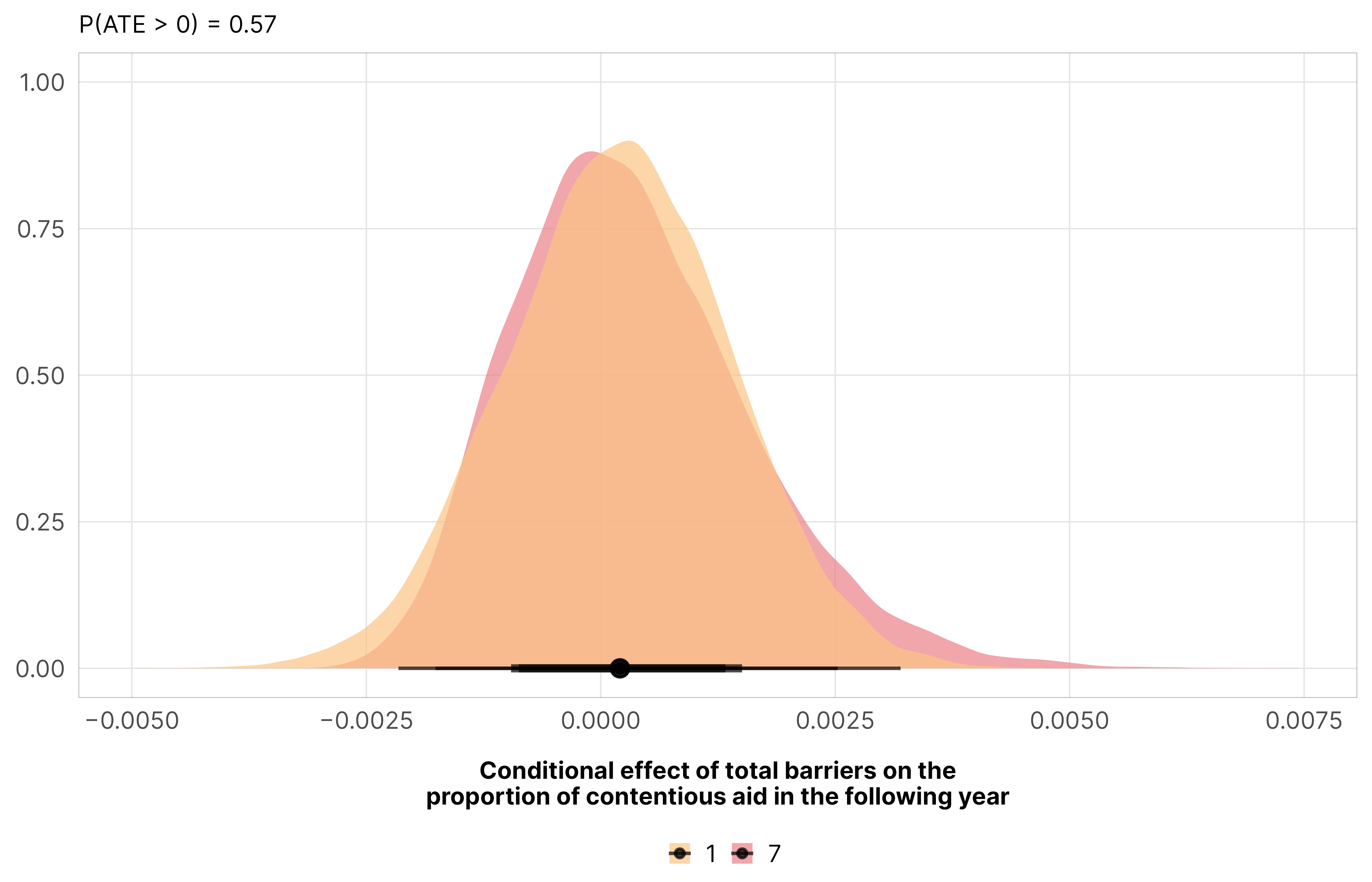
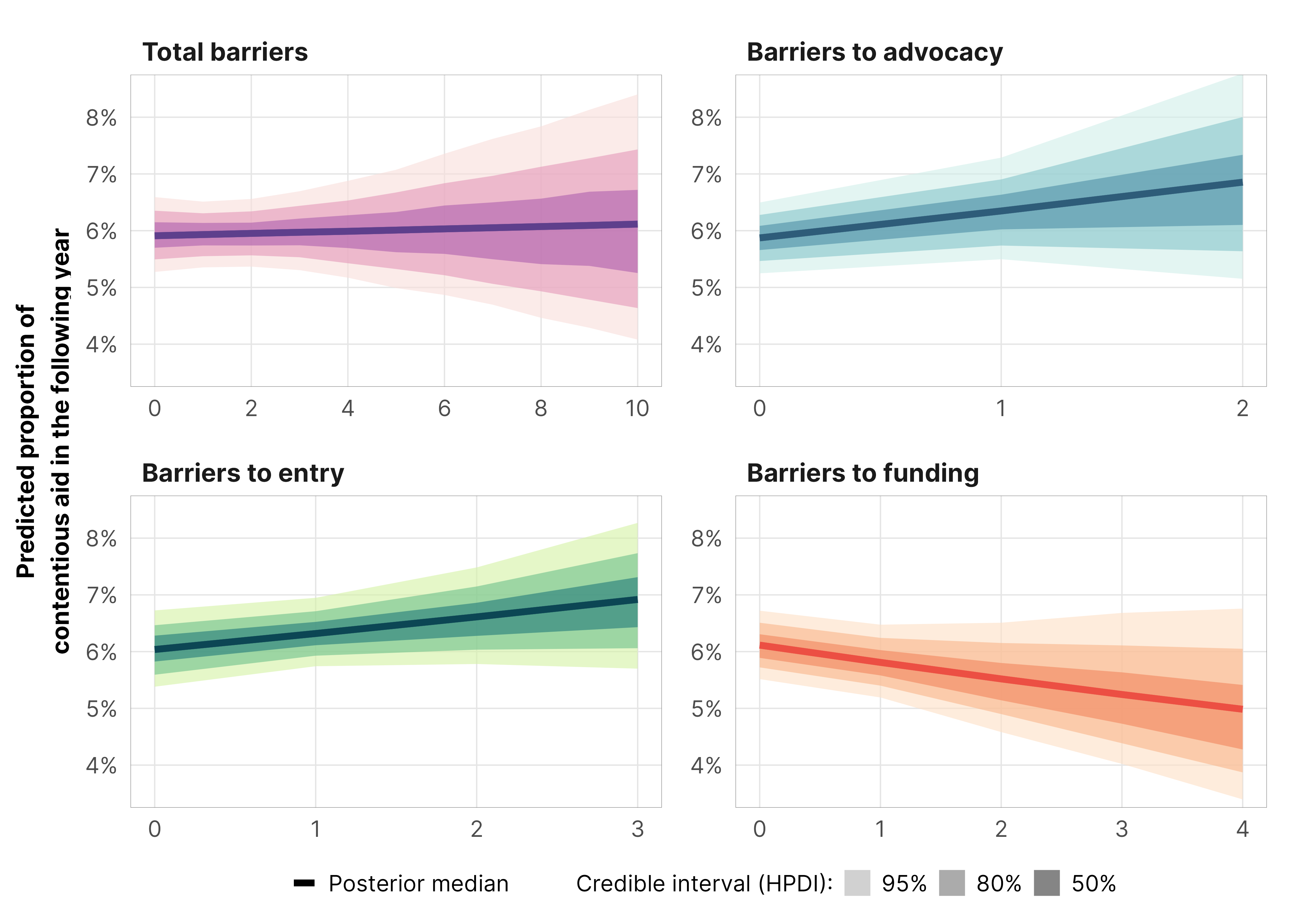
In this project we care most about conditional effects, or the effect of the treatment in a typical country, or effect of the treatment when all country-specific \(b_0\) and \(b_3\) estimates are set to 0.
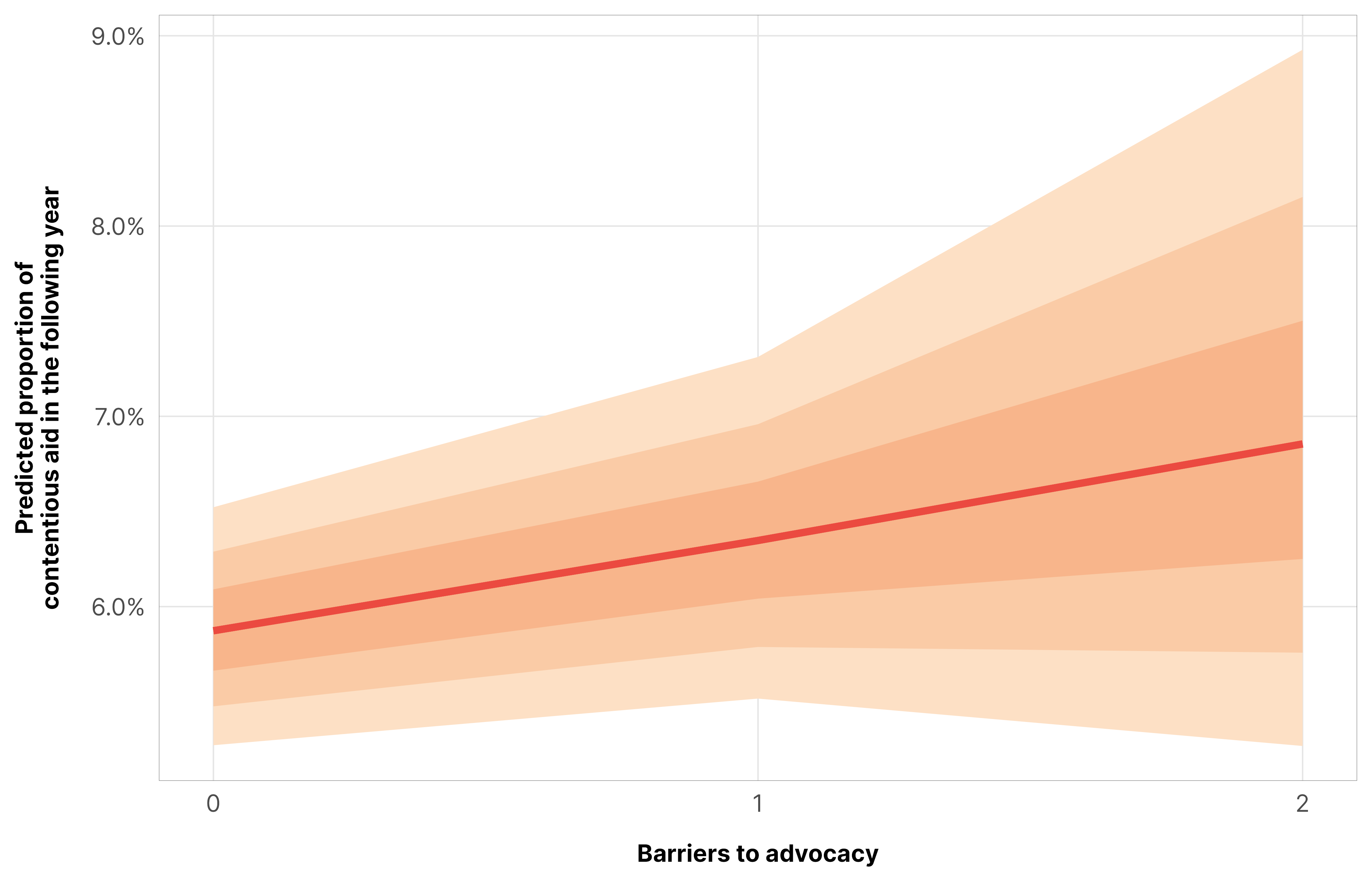
In general, contentious aid doesn’t really change at all as additional legal barriers are added. The slope of the line is 0.02 percentage points, with a credible interval that ranges between -0.2 and 0.25 percentage points. The effect is essentially zero.
Code
m_purpose_outcome_total$model %>%epred_draws(newdata =datagrid(model = m_purpose_outcome_total$model,year_c =0,barriers_total =seq(0, 10, 1)),re_formula =NA) %>%ggplot(aes(x = barriers_total, y = .epred)) +stat_lineribbon(color = clrs$Peach[7]) +scale_x_continuous(breaks =seq(0, 10, by =2)) +scale_y_continuous(labels =label_percent()) +scale_fill_manual(values = clrs$Peach[1:3]) +guides(fill ="none") +labs(x ="Total barriers", y ="Predicted proportion of\ncontentious aid in the following year") +theme_donors()
mfx_purpose_cfx_multiple$total %>%posteriordraws() %>%filter(barriers_total %in%c(1, 7)) %>%pivot_longer(draw) %>%ggplot(aes(x = value, fill =factor(barriers_total))) +stat_halfeye(alpha =0.7) +scale_x_continuous(labels =label_number(style_negative ="minus")) +scale_fill_manual(values = clrs$Sunset[c(2, 4, 6)]) +labs(x ="Conditional effect of total barriers on the\nproportion of contentious aid in the following year", y =NULL,subtitle =glue("P(ATE > 0) = {1 - pull(mfx_total_p_direction, pd_short)}"), fill =NULL) +theme_donors()
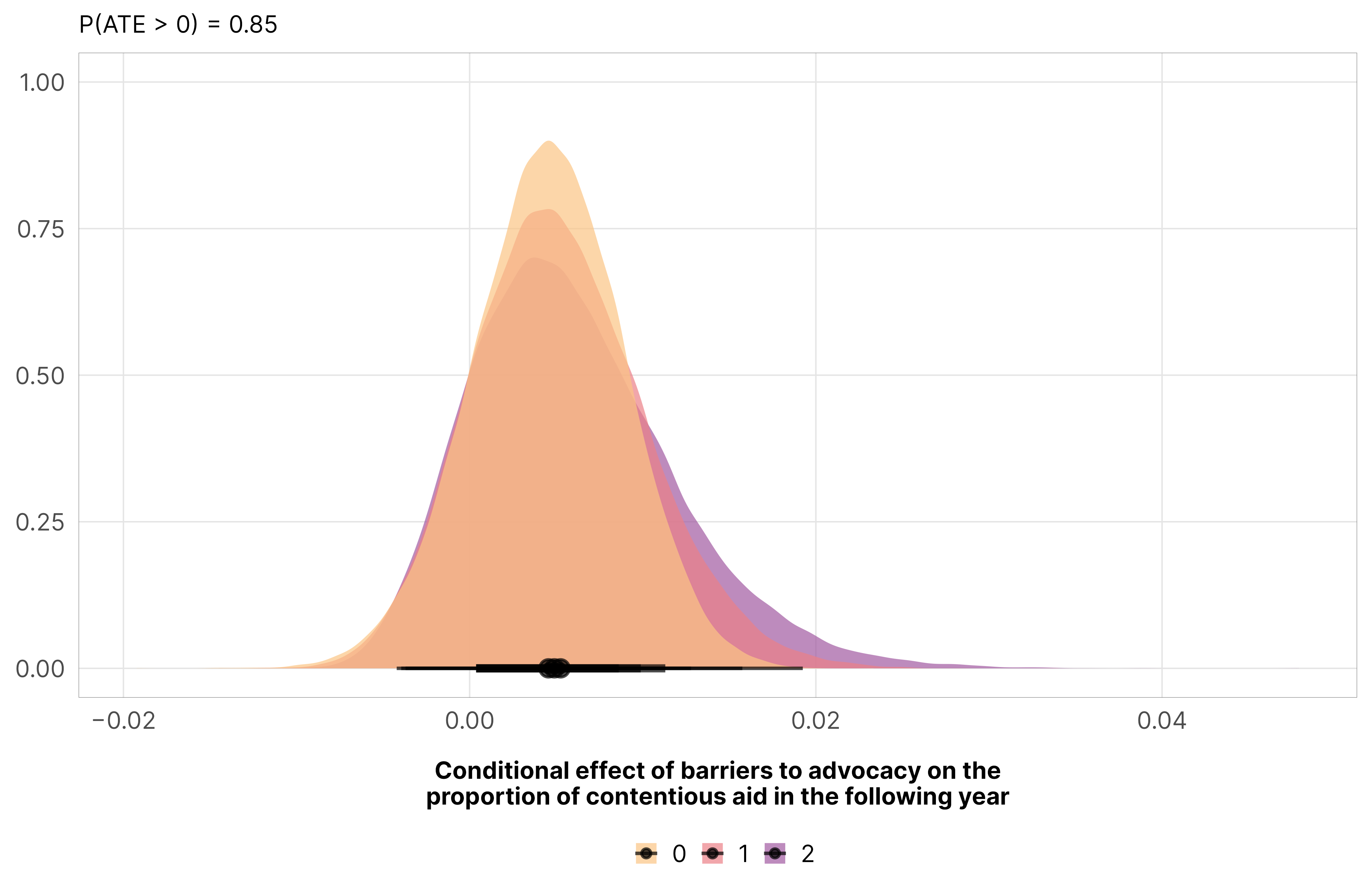
Contentious aid increases a little in response to restrictions on advocacy. The marginal effect when moving from 1 to 2 advocacy restrictions is half a percentage point, and the probability that it’s greater than zero is 0.85.
Code
m_purpose_outcome_advocacy$model %>%epred_draws(newdata =datagrid(model = m_purpose_outcome_advocacy$model,year_c =0,advocacy =seq(0, 2, 1)),re_formula =NA) %>%ggplot(aes(x = advocacy, y = .epred)) +stat_lineribbon(color = clrs$Peach[7]) +scale_x_continuous(breaks =0:2) +scale_y_continuous(labels =label_percent()) +scale_fill_manual(values = clrs$Peach[1:3]) +guides(fill ="none") +labs(x ="Barriers to advocacy", y ="Predicted proportion of\ncontentious aid in the following year") +theme_donors()
mfx_purpose_cfx_multiple$advocacy %>%posteriordraws() %>%pivot_longer(draw) %>%ggplot(aes(x = value, fill =factor(advocacy))) +stat_halfeye(alpha =0.7) +scale_x_continuous(labels =label_number(style_negative ="minus")) +scale_fill_manual(values = clrs$Sunset[c(2, 4, 6)]) +labs(x ="Conditional effect of barriers to advocacy on the\nproportion of contentious aid in the following year", y =NULL,subtitle =glue("P(ATE > 0) = {pull(mfx_advocacy_p_direction, pd_short)}"), fill =NULL) +theme_donors()
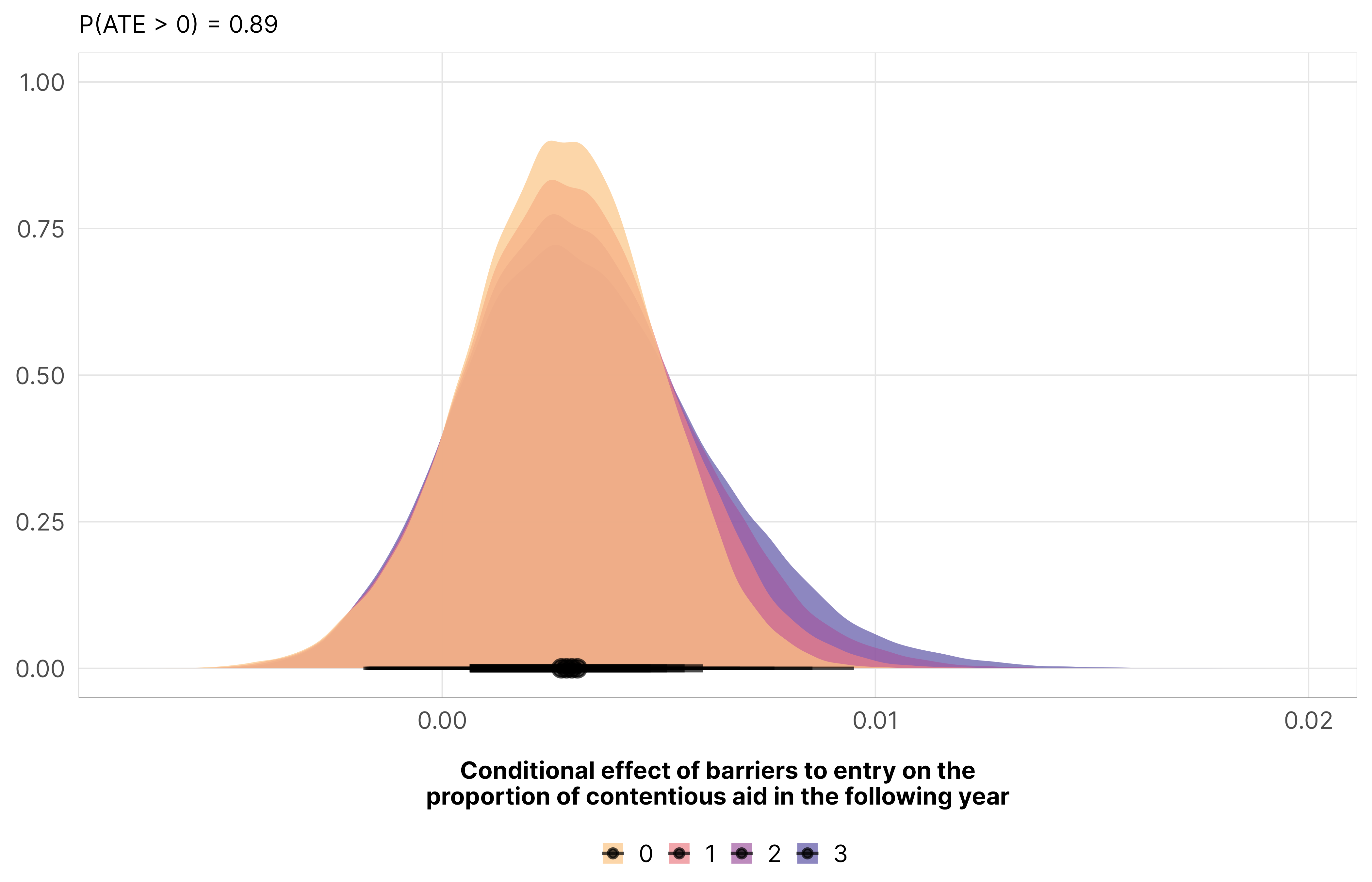
Contentious aid increases a little in response to restrictions on entry. The marginal effect is 0.3 percentage points, and the probability that it’s greater than zero is 0.89.
Code
m_purpose_outcome_entry$model %>%epred_draws(newdata =datagrid(model = m_purpose_outcome_entry$model,year_c =0,entry =seq(0, 3, 1)),re_formula =NA) %>%ggplot(aes(x = entry, y = .epred)) +stat_lineribbon(color = clrs$Peach[7]) +scale_x_continuous(breaks =0:3) +scale_y_continuous(labels =label_percent()) +scale_fill_manual(values = clrs$Peach[1:3]) +guides(fill ="none") +labs(x ="Barriers to entry", y ="Predicted proportion of\ncontentious aid in the following year") +theme_donors()
mfx_purpose_cfx_multiple$entry %>%posteriordraws() %>%pivot_longer(draw) %>%ggplot(aes(x = value, fill =factor(entry))) +stat_halfeye(alpha =0.7) +scale_x_continuous(labels =label_number(style_negative ="minus")) +scale_fill_manual(values = clrs$Sunset[c(2, 4, 6, 7)]) +labs(x ="Conditional effect of barriers to entry on the\nproportion of contentious aid in the following year", y =NULL,subtitle =glue("P(ATE > 0) = {pull(mfx_entry_p_direction, pd_short)}"), fill =NULL) +theme_donors()
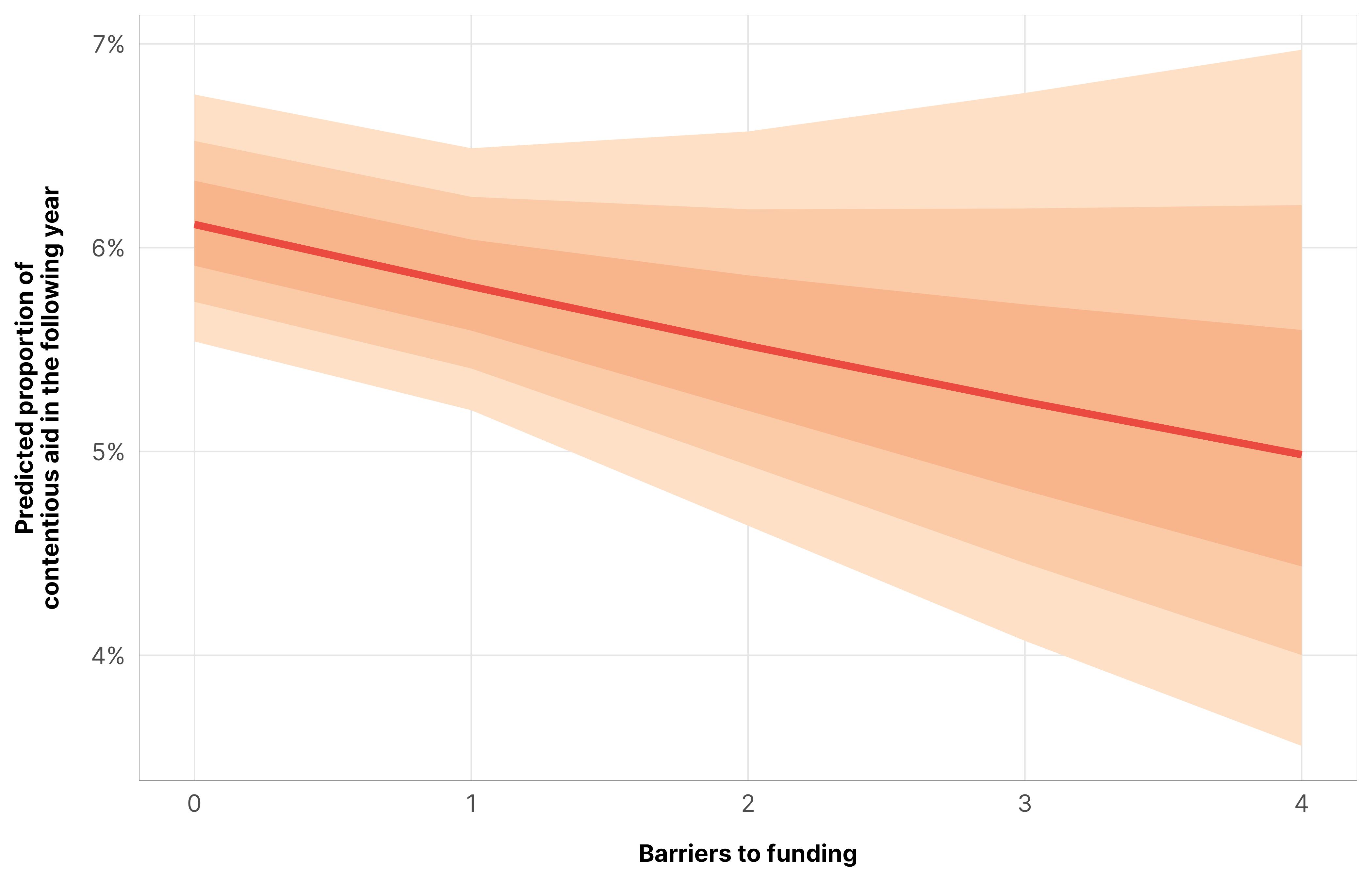
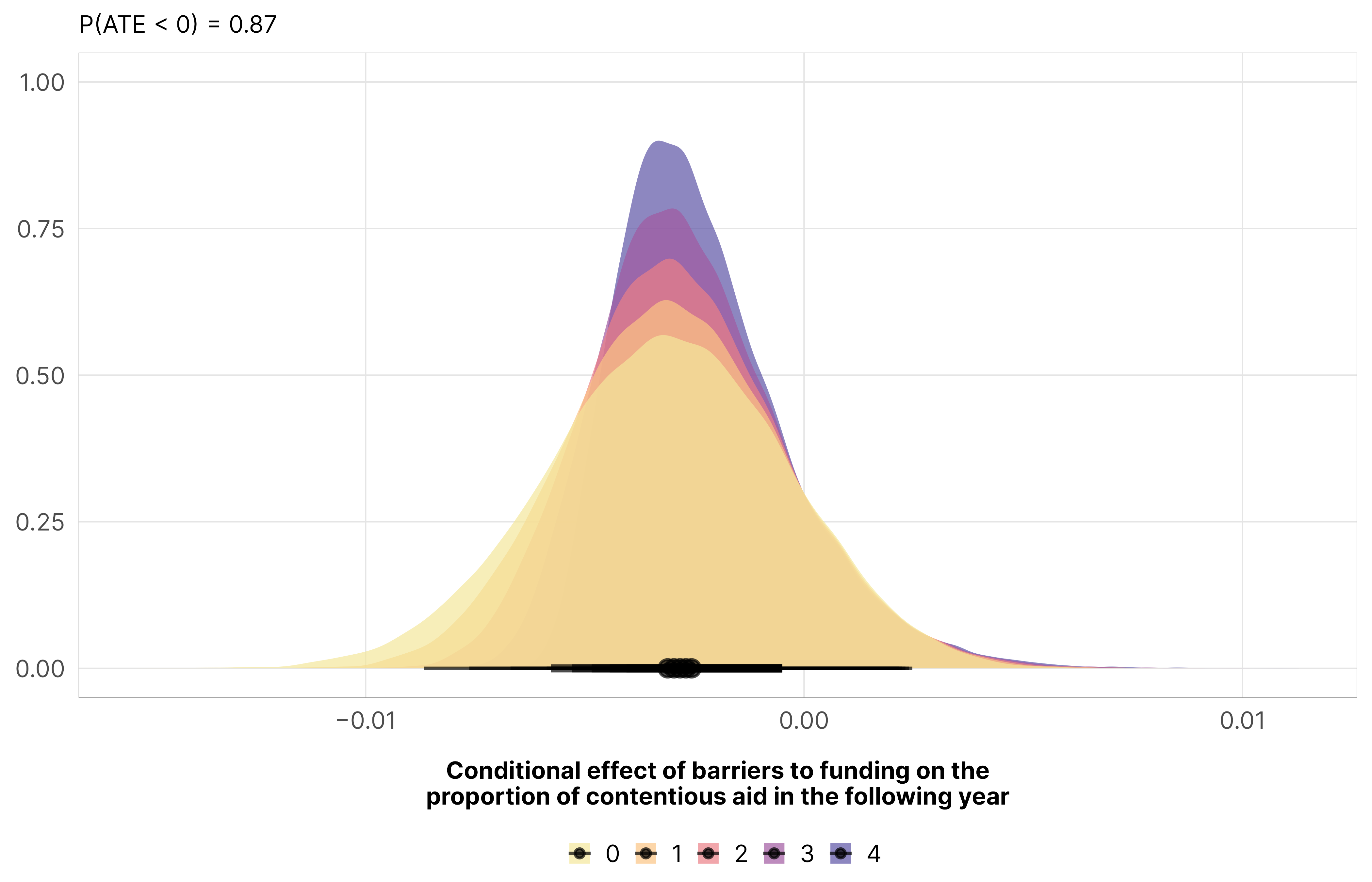
Contentious aid decreases a little in response to restrictions on funding. The marginal effect is -0.3 percentage points, and the probability that it’s less than 0 is 0.87.
Code
m_purpose_outcome_funding$model %>%epred_draws(newdata =datagrid(model = m_purpose_outcome_funding$model,year_c =0,funding =seq(0, 4, 1)),re_formula =NA) %>%ggplot(aes(x = funding, y = .epred)) +stat_lineribbon(color = clrs$Peach[7]) +scale_x_continuous(breaks =0:4) +scale_y_continuous(labels =label_percent()) +scale_fill_manual(values = clrs$Peach[1:3]) +guides(fill ="none") +labs(x ="Barriers to funding", y ="Predicted proportion of\ncontentious aid in the following year") +theme_donors()
mfx_purpose_cfx_multiple$funding %>%posteriordraws() %>%pivot_longer(draw) %>%ggplot(aes(x = value, fill =factor(funding))) +stat_halfeye(alpha =0.7) +scale_x_continuous(labels =label_number(style_negative ="minus")) +scale_fill_manual(values = clrs$Sunset[c(1, 2, 4, 6, 7)]) +labs(x ="Conditional effect of barriers to funding on the\nproportion of contentious aid in the following year", y =NULL,subtitle =glue("P(ATE < 0) = {pull(mfx_funding_p_direction, pd_short)}"), fill =NULL) +theme_donors()
Contentious aid doesn’t do much in response to changes in the de facto civil society environment. The official marginal effect is 0.01 percentage points (basically zero!) and the probability that it’s greater than zero is only 0.64.
Code
m_purpose_outcome_ccsi$model_50 %>%epred_draws(newdata =datagrid(model = m_purpose_outcome_ccsi$model_50,year_c =0,v2xcs_ccsi =seq(0, 1, 0.1)),re_formula =NA) %>%ggplot(aes(x = v2xcs_ccsi, y = .epred)) +stat_lineribbon(color = clrs$Peach[7]) +scale_x_reverse() +scale_y_continuous(labels =label_percent()) +scale_fill_manual(values = clrs$Peach[1:3]) +guides(fill ="none") +labs(x ="Core civil society index", y ="Predicted proportion of\ncontentious aid in the following year",caption ="**x-axis reversed**; lower values represent worse respect for civil society") +theme_donors() +theme(plot.caption =element_markdown())
mfx_purpose_cfx_multiple$ccsi %>%posteriordraws() %>%mutate(draw =-draw) %>%pivot_longer(draw) %>%ggplot(aes(x = value, fill =factor(v2xcs_ccsi))) +stat_halfeye(alpha =0.7) +scale_x_continuous(labels =label_number(style_negative ="minus")) +scale_fill_manual(values = clrs$Sunset[c(1, 2, 4, 6, 7)]) +labs(x ="Conditional effect of worsening the\ncore civil society index on contentious aid in the following year", y =NULL,subtitle =glue("P(ATE < 0) = {1 - pull(mfx_ccsi_p_direction, pd_short)}"), fill =NULL) +theme_donors()
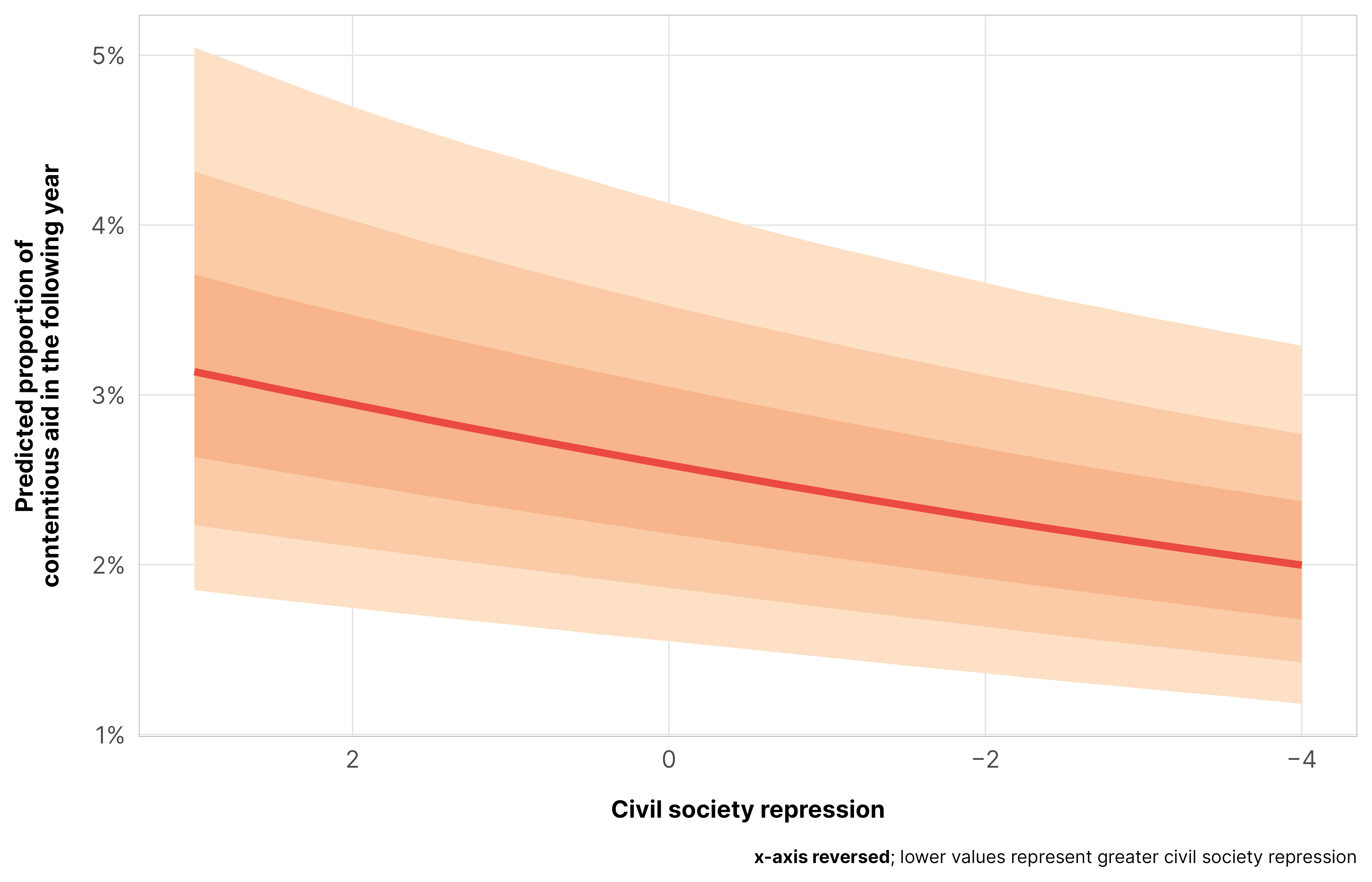
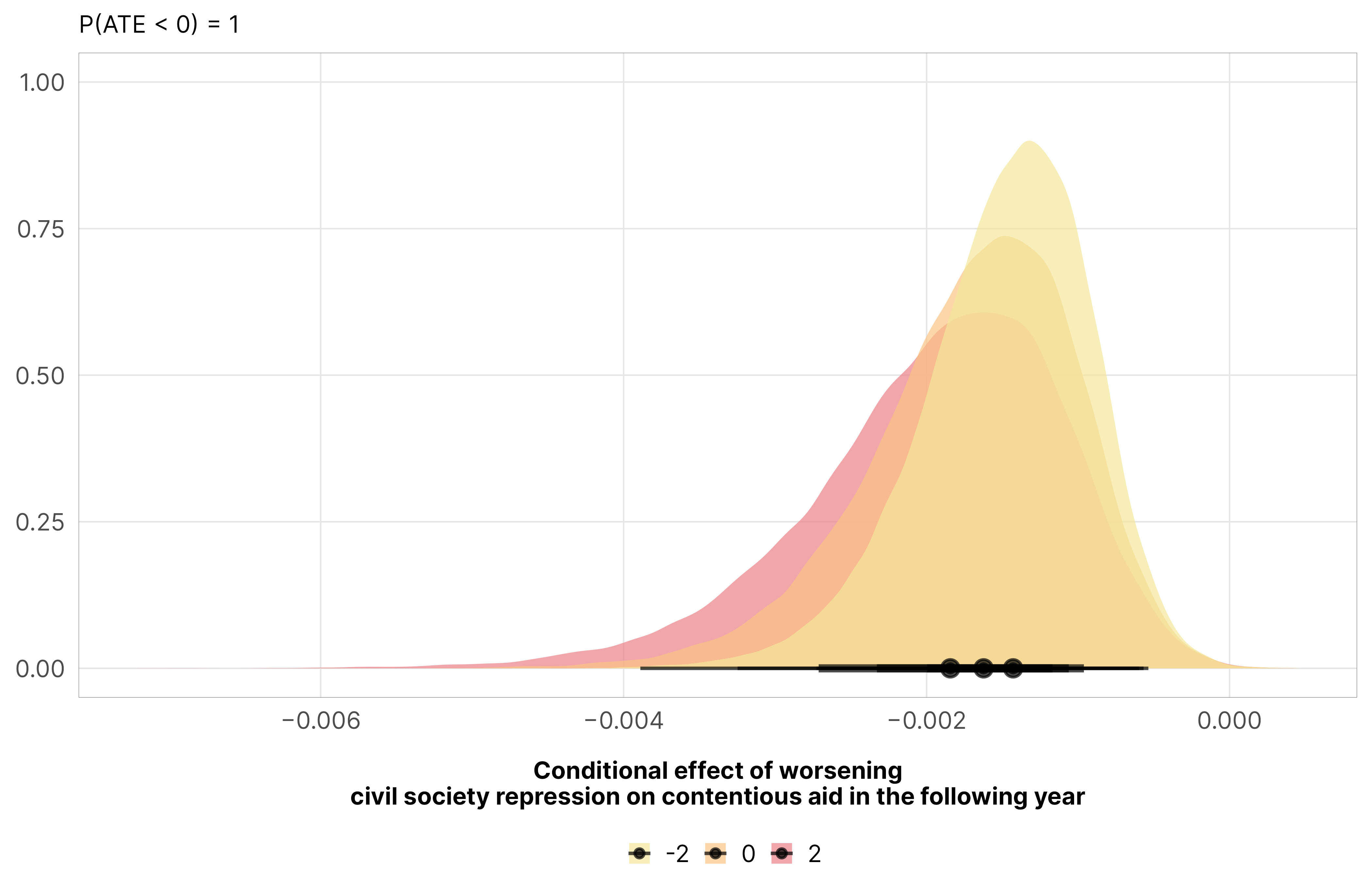
However, contentious aid increases as repression decreases or improves a little (0.16 percentage points, with a 100% probability of being greater than zero). Or in reverse, as civil society gets worse, contentious aid decreases (following Bush (2015)). This is interesting since it’s the opposite-ish for de jure restrictions—when barriers to advocacy and entry are enacted, contentious aid increases a little bit. But when the practical lived level of civil society repression increases, contentious aid drops.
Code
m_purpose_outcome_repress$model_50 %>%epred_draws(newdata =datagrid(model = m_purpose_outcome_repress$model_50,year_c =0,v2csreprss =seq(-4, 3, 0.25)),re_formula =NA) %>%ggplot(aes(x = v2csreprss, y = .epred)) +stat_lineribbon(color = clrs$Peach[7]) +scale_x_reverse(labels =label_number(style_negative ="minus")) +scale_y_continuous(labels =label_percent()) +scale_fill_manual(values = clrs$Peach[1:3]) +guides(fill ="none") +labs(x ="Civil society repression", y ="Predicted proportion of\ncontentious aid in the following year",caption ="**x-axis reversed**; lower values represent greater civil society repression") +theme_donors() +theme(plot.caption =element_markdown())
mfx_purpose_cfx_multiple$repress %>%posteriordraws() %>%mutate(draw =-draw) %>%pivot_longer(draw) %>%ggplot(aes(x = value, fill =factor(v2csreprss))) +stat_halfeye(alpha =0.7) +scale_x_continuous(labels =label_number(style_negative ="minus")) +scale_fill_manual(values = clrs$Sunset[c(1, 2, 4, 6, 7)]) +labs(x ="Conditional effect of worsening\ncivil society repression on contentious aid in the following year", y =NULL,subtitle =glue("P(ATE < 0) = {1 - pull(mfx_repress_p_direction, pd_short)}"), fill =NULL) +theme_donors()
# Put the shared y-axis label in a separate plot and add it to the combined plot# https://stackoverflow.com/a/66778622/120898p_lab <-ggplot() +annotate(geom ="text", x =1, y =1, angle =90, size =3.3, fontface ="bold",label ="Predicted proportion of\ncontentious aid in the following year") +coord_cartesian(clip ="off") +theme_void()(p_lab | ((p1 | p2) / (p3 | p4) +plot_layout(guides ="collect") +plot_annotation(theme =theme(legend.position ="bottom")))) +plot_layout(widths =c(0.05, 1))
The effect of de jure anti-NGO legal barriers on the predicted proportion of contentious aid in a typical country
Code
p1 <- m_purpose_outcome_ccsi$model_50 %>%epred_draws(newdata =datagrid(model = m_purpose_outcome_ccsi$model_50,year_c =0,v2xcs_ccsi =seq(0, 1, 0.1)),re_formula =NA) %>%ggplot(aes(x = v2xcs_ccsi, y = .epred)) +stat_lineribbon(aes(color ="Posterior median"), alpha =0.6, point_interval = median_hdci) +scale_x_reverse(breaks =seq(0, 1, by =0.25)) +scale_y_continuous(labels =label_percent(accuracy =1)) +scale_color_manual(values = clrs$Sunset[4],guide =guide_legend(order =1, override.aes =list(fill =NA, alpha =1, color ="black")) ) +scale_fill_manual(values = clrs$Sunset[c(1, 2, 3)], labels =function(x) label_percent()(as.numeric(x)),guide =guide_legend(order =2, override.aes =list(color =NA, fill = ci_cols)) ) +labs(x =NULL, y =NULL, color =NULL, fill ="Credible interval (HPDI):") +coord_cartesian(ylim =c(0.01, 0.05)) +facet_wrap(vars("Worsening core civil society index")) +theme_donors() +theme(legend.margin =margin(l =7.5, r =7.5))p2 <- m_purpose_outcome_repress$model_50 %>%epred_draws(newdata =datagrid(model = m_purpose_outcome_repress$model_50,year_c =0,v2csreprss =seq(-4, 3, 0.25)),re_formula =NA) %>%ggplot(aes(x = v2csreprss, y = .epred)) +stat_lineribbon(aes(color ="Posterior median"), alpha =0.6, point_interval = median_hdci) +scale_x_reverse(labels =label_number(style_negative ="minus")) +scale_y_continuous(labels =label_percent(accuracy =1)) +scale_color_manual(values = clrs$Sunset[7],guide =guide_legend(order =1, override.aes =list(fill =NA, alpha =1, color ="black")) ) +scale_fill_manual(values = clrs$Sunset[c(4, 5, 6)], labels =function(x) label_percent()(as.numeric(x)),guide =guide_legend(order =2, override.aes =list(color =NA, fill = ci_cols)) ) +labs(x =NULL, y =NULL, color =NULL, fill ="Credible interval (HPDI):",caption ="**x-axis reversed**; lower values represent worse respect for and repression of civil society") +coord_cartesian(ylim =c(0.01, 0.05)) +facet_wrap(vars("Worsening civil society repression")) +theme_donors() +theme(legend.margin =margin(l =7.5, r =7.5),plot.caption =element_markdown())p_lab <-ggplot() +annotate(geom ="text", x =1, y =1, angle =90, size =3.3, fontface ="bold",label ="Predicted proportion of\ncontentious aid in the following year") +coord_cartesian(clip ="off") +theme_void()(p_lab | ((p1 | p2) +plot_layout(guides ="collect") +plot_annotation(theme =theme(legend.position ="bottom")))) +plot_layout(widths =c(0.05, 1))
The effect of the de facto civil society legal environment on the predicted proportion of contentious aid in a typical country
p_lab <-ggplot() +annotate(geom ="text", x =1, y =1, size =3.3, fontface ="bold",label ="Conditional effect of treatment on proportion\nof contentious aid in the following year") +coord_cartesian(clip ="off") +theme_void()(((p1 | p2) / (p3 | p4)) / p_lab) +plot_layout(heights =c(1, 1, 0.2)) +plot_annotation(caption ="Point shows median value;\nthick bar = 80% credible interval; thin bar = 95% credible interval",theme =theme(plot.caption =element_text(family ="Inter")))
The effect of one additional de jure anti-NGO legal barrier on the predicted proportion of contentious aid in a typical country
Code
p1 <- mfx_purpose_cfx_single$ccsi %>%posteriordraws() %>%mutate(draw =-draw /10) %>%ggplot(aes(x = draw)) +stat_halfeye(aes(fill_ramp =after_stat(x <0)),fill = clrs$Sunset[4], .width =c(0.8, 0.95),point_interval = median_hdci) +geom_vline(xintercept =0, linewidth =0.25) +annotate(geom ="richtext", label =glue("P(ATE < 0) = {1 - pull(mfx_ccsi_stats, pd_short)}"),x =Inf, y =Inf, hjust =1, vjust =1, size =3,label.color =NA, label.margin =unit(rep(0.5, 4), "lines")) +scale_x_continuous(labels =label_number(scale =100, suffix =" pp.",style_negative ="minus")) +scale_fill_ramp_discrete(from = clrs$Sunset[3], guide ="none") +labs(x =NULL, y =NULL, fill =NULL) +facet_wrap(vars("A 0.1 unit decrease (worsening) in\nthe core civil society index")) +theme_donors() +theme(axis.text.y =element_blank())p2 <- mfx_purpose_cfx_single$repress %>%posteriordraws() %>%mutate(draw =-draw) %>%ggplot(aes(x = draw)) +stat_halfeye(aes(fill_ramp =after_stat(x >0)),fill = clrs$Sunset[6], .width =c(0.8, 0.95),point_interval = median_hdci) +geom_vline(xintercept =0, linewidth =0.25) +annotate(geom ="richtext", label =glue("P(ATE < 0) = {1 - pull(mfx_repress_stats, pd_short)}"),x =Inf, y =Inf, hjust =1, vjust =1, size =3,label.color =NA, label.margin =unit(rep(0.5, 4), "lines")) +scale_x_continuous(labels =label_number(scale =100, suffix =" pp.",style_negative ="minus")) +scale_fill_ramp_discrete(from = clrs$Sunset[3], guide ="none") +labs(x =NULL, y =NULL, fill =NULL) +facet_wrap(vars("A 1 unit decrease (worsening) in\nthe civil society repression score")) +theme_donors() +theme(axis.text.y =element_blank())p_lab <-ggplot() +annotate(geom ="text", x =1, y =1, size =3.3, fontface ="bold",label ="Conditional effect of treatment on proportion\nof contentious aid in the following year") +coord_cartesian(clip ="off") +theme_void()((p1 | p2) / p_lab) +plot_layout(heights =c(1, 0.15)) +plot_annotation(caption ="Point shows median value;\nthick bar = 80% credible interval; thin bar = 95% credible interval",theme =theme(plot.caption =element_text(family ="Inter")))
The effect of changes in the de facto civil society legal environment on the predicted proportion of contentious aid in a typical country
Table
With H1 we had to convert the dollar-scale treatment effects into percent changes to make them more interpretable, since we were working with millions of dollars. With this outcome, though, we’re just working with a 0–100% range, so we can stick with percentage point-scale effects.
Code
signif_pp <-label_number(accuracy =0.01, scale =100, suffix =" pp.",style_negative ="minus")signif_no_pp <-label_number(accuracy =0.01, scale =100,style_negative ="minus")mfx_lookup <-tribble(~term, ~Treatment,"barriers_total", "One additional barrier of any type","advocacy", "One additional barrier to advocacy","entry", "One additional barrier to entry","funding", "One additional barrier to funding","v2xcs_ccsi", "A 0.1 unit decrease in the core civil society index (i.e. worse environment)","v2csreprss", "A 1 unit decrease in the civil society repression score (i.e. more repression)") %>%mutate(Treatment =fct_inorder(Treatment))mfx_all_posteriors <-bind_rows(posteriordraws(mfx_purpose_cfx_single$total), posteriordraws(mfx_purpose_cfx_single$advocacy), posteriordraws(mfx_purpose_cfx_single$entry), posteriordraws(mfx_purpose_cfx_single$funding), (posteriordraws(mfx_purpose_cfx_single$ccsi) %>%mutate(draw = draw /10)),posteriordraws(mfx_purpose_cfx_single$repress)) %>%mutate(draw =ifelse(term %in%c("v2xcs_ccsi", "v2csreprss"), -draw, draw),dydx =ifelse(term %in%c("v2xcs_ccsi", "v2csreprss"), -dydx, dydx),conf.low_real =ifelse(term %in%c("v2xcs_ccsi", "v2csreprss"), -conf.high, conf.low),conf.high_real =ifelse(term %in%c("v2xcs_ccsi", "v2csreprss"), -conf.low, conf.high),conf.low = conf.low_real, conf.high = conf.high_real)mfx_p_direction <- mfx_all_posteriors %>%group_by(term) %>%summarize(pd_lt =round(sum(draw <0) /n(), 2),pd_gt =round(sum(draw >0) /n(), 2))mfx_medians <- mfx_all_posteriors %>%group_by(term) %>%median_hdci(draw) %>%left_join(mfx_p_direction, by ="term") %>%mutate(direction =case_when( draw >0~"more contentious aid in the next year", draw <0~"less contentious aid in the next year" )) %>%mutate(pd =case_when( draw >0~ pd_gt, draw <0~ pd_lt )) %>%mutate(pd_nice =label_percent(accuracy =1)(pd)) %>%mutate(across(c(draw, .upper), ~signif_pp(.))) %>%mutate(.lower =signif_no_pp(.lower)) %>%mutate(interval =glue("[{.lower}, {.upper}]")) %>%mutate(draw_nice =glue("{draw}\n{interval}")) %>%left_join(mfx_lookup, by ="term")mfx_medians_with_plots <- mfx_medians %>%group_by(term) %>%nest() %>%mutate(sparkplot =map(data, ~spark_bar(.x))) %>%mutate(sparkname =glue("sparkplots/contentiousness_bar_{term}")) %>%mutate(saved_plot =map2(sparkplot, sparkname, ~save_sparks(.x, .y)))mfx_median_clean <- mfx_medians_with_plots %>%ungroup() %>%select(-sparkplot) %>%unnest_wider(saved_plot) %>%unnest(data) %>%arrange(Treatment)
Code
tbl_notes <-c("The probability denotes the percentage of the posterior distribution that falls above or below 0.","Reported values are the median posterior marginal effect of each treatment variable on the outcome, multiplied by 100 to show percentage point changes; 95% highest posterior density intervals (HPDI) shown in brackets.")mfx_median_clean %>%mutate(Probability ="") %>%# mutate(across(c(draw.nice, pct_change.nice), ~linebreak(., align = "c"))) %>% # For LaTeXmutate(draw_nice =str_replace(draw_nice, "\\n", "<br>")) %>%select(Treatment, direction, Probability, draw_nice) %>%set_names(c(paste0("Probability", footnote_marker_symbol(1)),"Countries that add…", "…receive…", paste0("Median", footnote_marker_symbol(2)))) %>%kbl(align =c("l", "l", "l", "c"), escape =FALSE) %>%kable_styling(htmltable_class ="table table-sm table-borderless") %>%pack_rows("De jure legislation", 1, 4, indent =FALSE) %>%pack_rows("De facto enforcement", 5, 6, indent =FALSE) %>%column_spec(1, width ="34%") %>%column_spec(2, width ="34%") %>%column_spec(3, image = mfx_median_clean$png, width ="14%") %>%column_spec(4, width ="18%") %>%footnote(symbol = tbl_notes, footnote_as_chunk =FALSE)
Probability*
Countries that add…
…receive…
Median†
De jure legislation
One additional barrier of any type
more contentious aid in the next year
0.02 pp. [−0.21, 0.25 pp.]
One additional barrier to advocacy
more contentious aid in the next year
0.49 pp. [−0.43, 1.52 pp.]
One additional barrier to entry
more contentious aid in the next year
0.29 pp. [−0.19, 0.75 pp.]
One additional barrier to funding
less contentious aid in the next year
−0.30 pp. [−0.77, 0.21 pp.]
De facto enforcement
A 0.1 unit decrease in the core civil society index (i.e. worse environment)
less contentious aid in the next year
−0.01 pp. [−0.09, 0.05 pp.]
A 1 unit decrease in the civil society repression score (i.e. more repression)
less contentious aid in the next year
−0.16 pp. [−0.31, −0.05 pp.]
* The probability denotes the percentage of the posterior distribution that falls above or below 0.
† Reported values are the median posterior marginal effect of each treatment variable on the outcome, multiplied by 100 to show percentage point changes; 95% highest posterior density intervals (HPDI) shown in brackets.
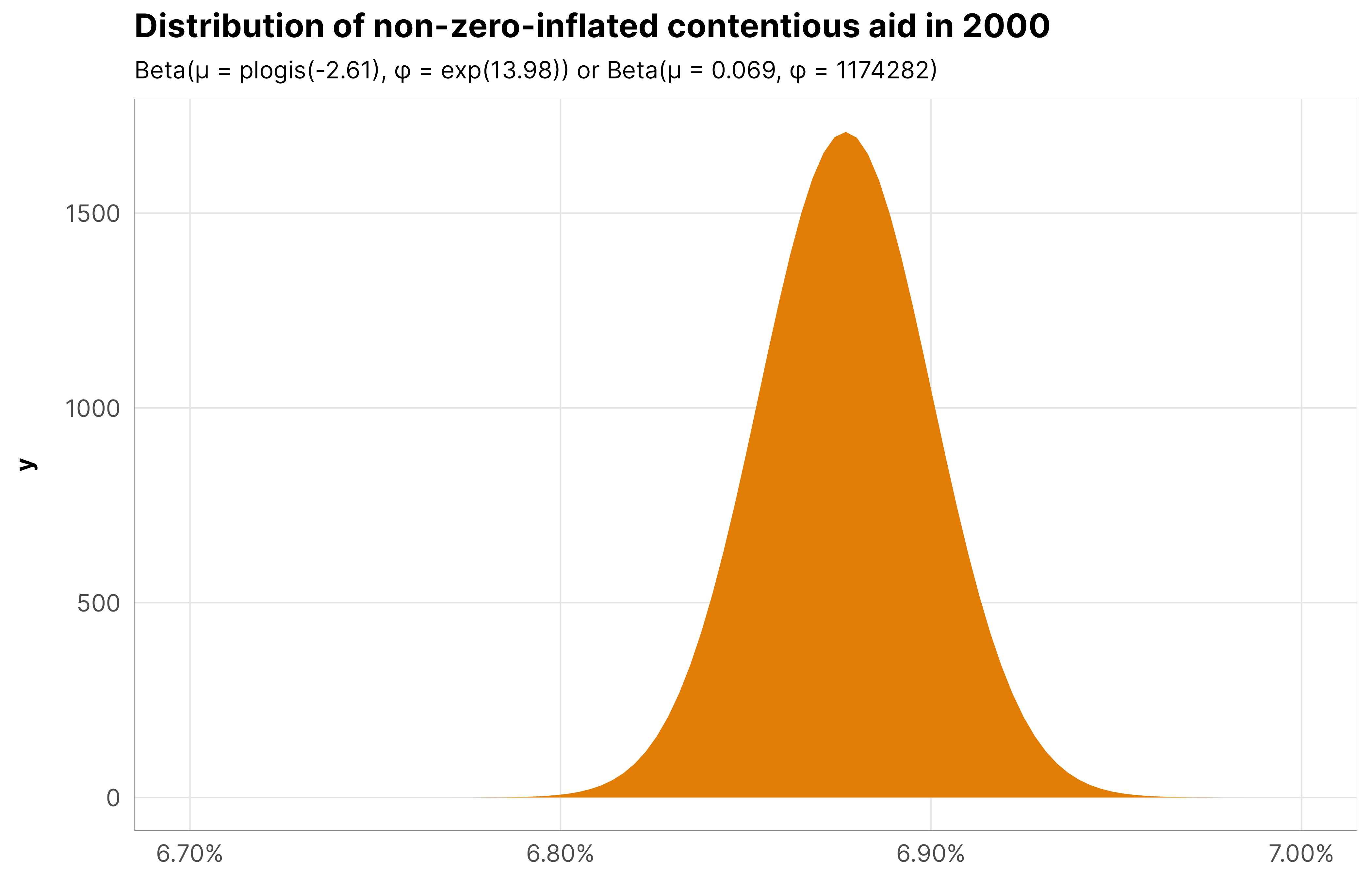
Within- and between-country variability (φ and σs)
The \(\phi\) and \(\sigma\) terms are roughly the same across all these different models, so we’ll just show the results from the total barriers model here. We have three uncertainty-related terms to work with:
\(\phi_y\) (phi): the precision or variance of aid contentiousness within countries. On the log scale, it’s 13.98, which is 1.174^{6} when unlogged or exponentiated, which is incredibly precise. That gives us a posterior distribution of the non-zero-inflated part of the model of \(\operatorname{Beta}(0.069, 1.174\times 10^{6})\) which looks like this, very narrowly focused around the baseline average 2000 proportion:
Code
beta_params <- m_purpose_outcome_total$model %>%tidy(parameters =c("b_(Intercept)", "phi"))beta_mu <- beta_params %>%filter(term =="b_(Intercept)") %>%pull(estimate)beta_phi <- beta_params %>%filter(term =="phi") %>%pull(estimate)ggplot() +stat_function(geom ="area", fill = clrs$Prism[7],fun =~dprop(., mean =plogis(beta_mu), size =exp(beta_phi))) +scale_x_continuous(labels =label_percent(), limits =c(0.067, 0.07)) +labs(title ="Distribution of non-zero-inflated contentious aid in 2000",subtitle = glue::glue("Beta(µ = plogis({round(beta_mu, 2)}), φ = exp({round(beta_phi, 2)})) or Beta(µ = {round(plogis(beta_mu), 3)}, φ = {round(exp(beta_phi), 0)})")) +theme_donors()
\(\sigma_0\) (sd__(Intercept) for the gwcode group): the variability between countries’ baseline averages, or the variability around the \(b_{0_j}\) offsets. Here it’s 0.55, which means that across or between countries, the proportion of contentious aid varies by 0.5ish logit units.
\(\sigma_3\) (sd__year_c for the gwcode group): the variability between countries’ year effects, or the variability around the \(b_{3_j}\) offsets. Here it’s 0.04, which means that average year effects vary by 0.04 logit units across or between countries.
Again, this is less important since we don’t care about individual coefficients and instead care about conditional effects, but for the sake of full transparency (and to placate future reviewers), here’s a table of all the results:
Code
models_tbl_h2_outcome_dejure <- models_tbl_h2_outcome_dejure %>%set_names(1:length(.))notes <-c("Posterior medians; 95% credible intervals (HDPI) in brackets.", "Total \\(R^2\\) considers the variance of both population and group effects;", "marginal \\(R^2\\) only takes population effects into account")modelsummary(models_tbl_h2_outcome_dejure,estimate ="{estimate}",statistic ="[{conf.low}, {conf.high}]",add_rows = outcome_rows,coef_map = coefs_outcome,gof_map = gofs,output ="kableExtra",fmt =list(estimate =2, conf.low =2, conf.high =2)) %>%row_spec(1, bold =TRUE) %>%kable_styling(htmltable_class ="table-sm light-border") %>%footnote(general = notes, footnote_as_chunk =TRUE)
Table 4: Results from all outcome models
1
2
3
4
Treatment
Total barriers (t)
Barriers to advocacy (t)
Barriers to entry (t)
Barriers to funding (t)
Treatment (t − 1)
0.004
0.08
0.05
−0.05
[−0.04, 0.05]
[−0.07, 0.24]
[−0.03, 0.13]
[−0.15, 0.04]
Treatment history
−0.006
−0.01
−0.01
−0.01
[−0.01, −0.002]
[−0.03, 0.001]
[−0.02, −0.001]
[−0.02, −0.0009]
Intercept
−2.61
−2.66
−2.59
−2.61
[−2.72, −2.49]
[−2.77, −2.55]
[−2.71, −2.47]
[−2.72, −2.51]
Year
0.07
0.07
0.07
0.07
[0.06, 0.09]
[0.06, 0.08]
[0.06, 0.08]
[0.06, 0.08]
Zero-inflated part: Year
−0.05
−0.03
−0.05
−0.05
[−0.06, −0.03]
[−0.05, −0.02]
[−0.06, −0.03]
[−0.06, −0.03]
Zero-inflated part: Year²
0.01
0.01
0.01
0.01
[0.01, 0.02]
[0.01, 0.02]
[0.01, 0.02]
[0.01, 0.02]
Zero-inflated part: Intercept
−2.57
−2.54
−2.50
−2.58
[−2.75, −2.40]
[−2.72, −2.36]
[−2.69, −2.32]
[−2.76, −2.41]
Between-country intercept variability (\(\sigma_0\) for \(b_0\) offsets)
0.55
0.55
0.52
0.53
[0.47, 0.64]
[0.47, 0.64]
[0.45, 0.61]
[0.45, 0.62]
Between-country year variability (\(\sigma_3\) for \(b_3\) offsets)
0.04
0.03
0.04
0.04
[0.03, 0.05]
[0.03, 0.04]
[0.03, 0.05]
[0.03, 0.05]
Correlation between random intercepts and slopes (\(\rho\))
0.15
0.19
0.22
0.14
[−0.11, 0.39]
[−0.09, 0.45]
[−0.03, 0.45]
[−0.12, 0.38]
Model dispersion (\(\phi_y\))
13.97
13.79
12.36
13.58
[13.18, 14.79]
[12.92, 14.70]
[11.59, 13.16]
[12.79, 14.39]
N
3151
3151
3151
3151
\(R^2\) (total)
0.30
0.26
0.30
0.30
\(R^2\) (marginal)
0.07
0.05
0.07
0.07
Note: Posterior medians; 95% credible intervals (HDPI) in brackets. Total \(R^2\) considers the variance of both population and group effects; marginal \(R^2\) only takes population effects into account
References
Bush, Sarah Sunn. 2015. The Taming of Democracy Assistance: Why Democracy Promotion Does Not Confront Dictators. Cambridge, UK: Cambridge University Press. https://doi.org/10.1017/cbo9781107706934.
Keele, Luke, Randolph T. Stevenson, and Felix Elwert. 2020. “The Causal Interpretation of Estimated Associations in Regression Models.”Political Science Research and Methods 8 (1): 1–13. https://doi.org/10.1017/psrm.2019.31.
McElreath, Richard. 2020. Statistical Rethinking: A Bayesian Course with Examples in R and Stan. 2nd ed. Boca Raton, Florida: Chapman and Hall / CRC.
Schielzeth, Holger. 2010. “Simple Means to Improve the Interpretability of Regression Coefficients.”Methods in Ecology and Evolution 1 (2): 103–13. https://doi.org/10.1111/j.2041-210X.2010.00012.x.
Westreich, Daniel, and Sander Greenland. 2013. “The Table 2 Fallacy: Presenting and Interpreting Confounder and Modifier Coefficients.”American Journal of Epidemiology 177 (4): 292–98. https://doi.org/10.1093/aje/kws412.
Source Code
---title: "H~2~: Effect of anti-NGO crackdown on aid contentiousness"format: html: code-fold: true toc-depth: 5 knitr: opts_chunk: out.width: "80%"editor_options: chunk_output_type: inline---```{r setup, include=FALSE}options(digits =3, width =120,dplyr.summarise.inform =FALSE,knitr.kable.NA ="")``````{r load-libraries-data, warning=FALSE, message=FALSE}library(tidyverse)library(targets)library(brms)library(tidybayes)library(broom)library(broom.mixed)library(modelsummary)library(marginaleffects)library(patchwork)library(scales)library(ggdist)library(ggtext)library(ggh4x)library(extraDistr)library(kableExtra)library(glue)library(here)tar_config_set(store = here::here('_targets'),script = here::here('_targets.R'))set.seed(1234)# Load stuff from targets# Plotting functionsinvisible(list2env(tar_read(graphic_functions), .GlobalEnv))invisible(list2env(tar_read(tbl_functions), .GlobalEnv))set_annotation_fonts()# Tell bayesplot to use the sunset palette for things like pp_check()bayesplot::color_scheme_set(clrs$Sunset[2:7])# Datadf_country_aid <-tar_read(country_aid_final)df_country_aid_laws <-filter(df_country_aid, laws)# Treatment modelstar_load(c(m_purpose_treatment_total, m_purpose_treatment_advocacy, m_purpose_treatment_entry, m_purpose_treatment_funding, m_purpose_treatment_ccsi, m_purpose_treatment_repress))# IPTW datatar_load(c(df_purpose_iptw_total, df_purpose_iptw_advocacy, df_purpose_iptw_entry, df_purpose_iptw_funding, df_purpose_iptw_ccsi, df_purpose_iptw_repress))# Outcome modelstar_load(c(m_purpose_outcome_total, m_purpose_outcome_advocacy, m_purpose_outcome_entry, m_purpose_outcome_funding, m_purpose_outcome_ccsi, m_purpose_outcome_repress))# Marginal/conditional effectstar_load(c(mfx_purpose_cfx_multiple, mfx_purpose_cfx_single))# Results tablestar_load(c(models_tbl_h2_treatment_num, models_tbl_h2_treatment_denom))tar_load(c(models_tbl_h2_outcome_dejure, models_tbl_h2_outcome_defacto))``````{r modelsummary-settings}invisible(list2env(tar_read(modelsummary_functions), .GlobalEnv))treatment_names <-c("Treatment", "Total barriers (t)", "Barriers to advocacy (t)", "Barriers to entry (t)", "Barriers to funding (t)", "CCSI (t)","CS repression (t)")treatment_rows <-as.data.frame(t(treatment_names))attr(treatment_rows, "position") <-1outcome_names <-c("Treatment", "Total barriers (t)", "Barriers to advocacy (t)", "Barriers to entry (t)", "Barriers to funding (t)")outcome_rows <-as.data.frame(t(outcome_names))attr(outcome_rows, "position") <-1```# Weight models## General ideaSee the ["Weight models—General idea" section from the total aid page](models_total-aid.qmd#general-idea) for an explanation of the intuition behind how to create these stabilized weights.## Actual modelsWe identify our time-varying and time-invariant confounders based on [our causal model and *do*-calculus logic](causal-model.qmd#final-variables-to-use), and we deal with the panel structure of the data by including random intercepts for country, and both a population-level trend and random slopes for year. We use [generic weakly informative priors](https://mc-stan.org/users/documentation/case-studies/weakly_informative_shapes.html) for our model parameters.### NumeratorOur numerator models look like this (but with the actual treatment variable replacing `treatment`, like `barriers_total`, `advocacy`, and so on):```{r fake-numerator, eval=FALSE}#| code-fold: showbf(treatment ~ treatment_lag1 + treatment_lag2_cumsum + (1| gwcode))```Or more formally:$$\begin{aligned}\text{Treatment}_{it_j} &\sim \mathcal{N}(\mu_{it_j}, \sigma_y) \\\mu_{it_j} &= (\beta_0 + b_{0_j}) + \beta_1 \text{Treatment}_{i, t-1_j} + \textstyle{\sum_{\tau = (t-2)}^{t}} \text{Treatment}_{i\tau} \\b_{0_j} &\sim \mathcal{N}(0, \sigma_0) \\\\\beta_0, \beta_1 &\sim \operatorname{Student~\textit{t}\,}(\nu = 3, \mu = 0, \sigma = 1.5) \\\sigma_y, \sigma_0 &\sim \operatorname{Exponential}(1)\end{aligned}$$### DenominatorOur denominator models look like this (but again with the actual treatment variable replacing `treatment`):```{r fake-denominator, eval=FALSE}#| code-fold: showbf(treatment ~ treatment_lag1 + treatment_lag2_cumsum +# Lagged outcome prop_contentious_lag1 +# Human rights and politics v2x_polyarchy + v2x_corr + v2x_rule + v2x_civlib + v2x_clphy + v2x_clpriv +# Economics and development gdpcap_log_z + un_trade_pct_gdp + v2peedueq + v2pehealth + e_peinfmor +# Conflict and disasters internal_conflict_past_5 + natural_dis_count +# Time and country effects year_c + (1+ year_c | gwcode))```Or more formally:$$\begin{aligned}\text{Treatment}_{it_j} \sim&\ \mathcal{N}(\mu_{it_j}, \sigma_y) \\\mu_{it_j} =&\ (\beta_0 + b_{0_j}) + \beta_1\, \text{Treatment}_{i, t-1_j} + \beta_2\, \textstyle{\sum_{\tau = (t-2)}^{t}} \text{Treatment}_{i\tau} + \\&\ \beta_3\, \text{Proportion of contentious aid}_{i,t-1_j} + \beta_{4 \ldots 9}\, \text{Human rights \& politics}_{it_j} + \\&\ \beta_{10 \ldots 14}\, \text{Economics \& development} + \beta_{15, 16}\, \text{Conflict \& disasters}_{it_j} + \\&\ (\beta_{17} + b_{17_j})\, \text{Year}_{it_j} \\\left( \begin{array}{c} b_{0_j} \\ b_{17_j} \end{array}\right) \sim&\ \text{MV}\,\mathcal{N}\left[ \left( \begin{array}{c} 0 \\ 0 \\ \end{array} \right) , \, \left( \begin{array}{cc} \sigma^2_{0} & \rho_{0, 17}\, \sigma_{0} \sigma_{17} \\ \cdots & \sigma^2_{17} \end{array}\right)\right] \\\\\beta_0 \ldots \beta_{17} \sim&\ \operatorname{Student~\textit{t}\,}(\nu = 3, \mu = 0, \sigma = 1.5) \\\sigma_y, \sigma_0, \sigma_{17} \sim&\ \operatorname{Exponential}(1) \\\rho \sim&\ \operatorname{LKJ}(2)\end{aligned}$$## MCMC diagnosticsAgain, as a check to make sure these weight models converged, here are some visual diagnostics for the total barriers treatment. All the other models look basically the same as these.### Numerator::: {.panel-tabset}#### Trace plots```{r plot-num-trace, warning=FALSE}#| out-width: 80%m_purpose_treatment_total$model_num %>%gather_draws(`^b_.*|^sd_.*|^sigma`, regex =TRUE) %>%ggplot(aes(x = .iteration, y = .value, color =factor(.chain))) +geom_line(linewidth =0.1) +scale_color_manual(values = clrs$Sunset[3:6]) +facet_wrap(vars(.variable), scales ="free_y") +theme_donors()```#### Trank plots```{r plot-num-trank, warning=FALSE}#| out-width: 80%m_purpose_treatment_total$model_num %>%gather_draws(`^b_.*|^sd_.*|^sigma`, regex =TRUE) %>%group_by(.variable) %>%mutate(draw_rank =rank(.value)) %>%ggplot(aes(x = draw_rank, color =factor(.chain))) +stat_bin(geom ="step", binwidth =500, position =position_identity(), boundary =0) +scale_color_manual(values = clrs$Sunset[3:6]) +facet_wrap(vars(.variable), scales ="free_y") +theme_donors() +theme(axis.text.y =element_blank(), axis.title.y =element_blank(), axis.ticks.y =element_blank())```#### Posterior predictive check```{r plot-num-ppcheck}#| out-width: 80%withr::with_seed(1234, {pp_check(m_purpose_treatment_total$model_num, ndraws =20) +labs(x ="Total NGO barriers",title ="Numerator model") +theme_donors()})```:::### Denominator::: {.panel-tabset}#### Trace plots```{r plot-denom-trace, warning=FALSE, fig.width=10, fig.height=7}#| out-width: 100%m_purpose_treatment_total$model_denom %>%gather_draws(`^b_.*|^sd_.*|^cor_.*|^sigma`, regex =TRUE) %>%ggplot(aes(x = .iteration, y = .value, color =factor(.chain))) +geom_line(linewidth =0.1) +scale_color_manual(values = clrs$Sunset[3:6]) +facet_wrap(vars(.variable), scales ="free_y") +theme_donors()```#### Trank plots```{r plot-denom-trank, warning=FALSE, fig.width=10, fig.height=7}#| out-width: 100%m_purpose_treatment_total$model_denom %>%gather_draws(`^b_.*|^sd_.*|^cor_.*|^sigma`, regex =TRUE) %>%group_by(.variable) %>%mutate(draw_rank =rank(.value)) %>%ggplot(aes(x = draw_rank, color =factor(.chain))) +stat_bin(geom ="step", binwidth =500, position =position_identity(), boundary =0) +scale_color_manual(values = clrs$Sunset[3:6]) +facet_wrap(vars(.variable), scales ="free_y") +theme_donors() +theme(axis.text.y =element_blank(), axis.title.y =element_blank(), axis.ticks.y =element_blank())```#### Posterior predictive check```{r plot-denom-ppcheck}#| out-width: 80%withr::with_seed(1234, {pp_check(m_purpose_treatment_total$model_denom, ndraws =20) +labs(x ="Total NGO barriers",title ="Denominator model") +theme_donors()})```:::## Check weightsAgain, IPTWs should generally have a mean of 1 and shouldn't be too incredibly high.::: {.panel-tabset}### Total barriersThe max weight here is `r round(max(df_purpose_iptw_total$iptw), 0)`, but as with H~1~ there are only a few observations with weights that high. The average is `r round(mean(df_purpose_iptw_total$iptw), 2)` and the median is `r round(median(df_purpose_iptw_total$iptw), 2)`, which are both close to 1, which is good.```{r iptws-total-purpose}#| code-fold: showsummary(df_purpose_iptw_total$iptw)``````{r plot-iptws-total-purpose}df_purpose_iptw_total %>%ggplot(aes(x = iptw)) +geom_histogram(binwidth =0.5, boundary =0) +theme_donors()```### AdvocacyThe max weight here is `r round(max(df_purpose_iptw_advocacy$iptw), 0)`, and the average is `r round(mean(df_purpose_iptw_advocacy$iptw), 2)`, so we're good still.```{r iptws-advocacy}#| code-fold: showsummary(df_purpose_iptw_advocacy$iptw)``````{r plot-iptws-advocacy}df_purpose_iptw_advocacy %>%ggplot(aes(x = iptw)) +geom_histogram(binwidth =0.5, boundary =0) +theme_donors()```### EntryThe max weight here is `r round(max(df_purpose_iptw_entry$iptw), 0)` and the average is `r round(mean(df_purpose_iptw_entry$iptw), 2)`, so everything's still great.```{r iptws-entry}#| code-fold: showsummary(df_purpose_iptw_entry$iptw)``````{r plot-iptws-entry}df_purpose_iptw_entry %>%ggplot(aes(x = iptw)) +geom_histogram(binwidth =0.5, boundary =0) +theme_donors()```### FundingThe max weight is `r round(max(df_purpose_iptw_funding$iptw), 0)` and the average is `r round(mean(df_purpose_iptw_funding$iptw), 2)`—great!```{r iptws-funding}#| code-fold: showsummary(df_purpose_iptw_funding$iptw)``````{r plot-iptws-funding}df_purpose_iptw_funding %>%ggplot(aes(x = iptw)) +geom_histogram(binwidth =0.5, boundary =0) +theme_donors()```### Core civil society indexlol these blow up again; the max weight is `r label_comma()(max(df_purpose_iptw_ccsi$iptw))`.```{r iptws-ccsi}#| code-fold: showsummary(df_purpose_iptw_ccsi$iptw)```There aren't a lot of observations with weights that high though—only 100ish:```{r show-threshold-counts-iptws-ccsi}#| code-fold: showdf_purpose_iptw_ccsi %>%count(iptw >=50)df_purpose_iptw_ccsi %>%count(iptw >=500)```We truncate these weights at 50.```{r plot-iptws-ccsi}plot_iptw_ccsi <-bind_rows( df_purpose_iptw_ccsi %>%mutate(threshold =50, iptw =ifelse(iptw > threshold, threshold, iptw)), df_purpose_iptw_ccsi %>%mutate(threshold =500, iptw =ifelse(iptw > threshold, threshold, iptw))) %>%mutate(threshold =paste0("Truncated at ", threshold),threshold =fct_inorder(threshold))plot_iptw_ccsi %>%ggplot(aes(x = iptw)) +geom_histogram(bins =50, boundary =0) +facet_wrap(vars(threshold), scales ="free_x") +theme_donors()```### Civil society repressionThese weights are also horrendous, with a maximum weight of `r label_comma()(max(df_purpose_iptw_repress$iptw))`.```{r iptws-csrepress}#| code-fold: showsummary(df_purpose_iptw_repress$iptw)```As with the core civil society index, there aren't a lot of observations with weights that high:```{r show-threshold-counts-iptws-csrepress}#| code-fold: showdf_purpose_iptw_repress %>%count(iptw >=50)df_purpose_iptw_repress %>%count(iptw >=500)```So we truncate these weights at 50 again. Since the results from the core civil society models are basically the same when truncating at 500, we only use a truncation point of 50 here.```{r plot-iptws-csrepress}df_purpose_iptw_ccsi %>%mutate(threshold =50, iptw =ifelse(iptw > threshold, threshold, iptw)) %>%ggplot(aes(x = iptw)) +geom_histogram(bins =50, boundary =0) +theme_donors()```:::## ResultsThese are less important since we just use these treatment models to generate weights *and* because interpreting each coefficient when trying to isolate causal effects is unimportant [@WestreichGreenland:2013; @KeeleStevensonElwert:2020].::: {.panel-tabset}### Numerator```{r tbl-h2-num, warning=FALSE}#| tbl-cap: Results from all numerator modelsmodels_tbl_h2_treatment_num <- models_tbl_h2_treatment_num %>%set_names(1:length(.))notes <-c("Posterior medians; 95% credible intervals in brackets", "Total \\(R^2\\) considers the variance of both population and group effects", "Marginal \\(R^2\\) only takes population effects into account")modelsummary(models_tbl_h2_treatment_num,estimate ="{estimate}",statistic ="[{conf.low}, {conf.high}]",add_rows = treatment_rows,coef_map = coefs_num,gof_map = gofs,output ="kableExtra",fmt =list(estimate =2, conf.low =2, conf.high =2)) %>%row_spec(1, bold =TRUE) %>%kable_styling(htmltable_class ="table-sm light-border")```### Denominator```{r tbl-h2-denom, warning=FALSE}#| tbl-cap: Results from all numerator modelsmodels_tbl_h2_treatment_denom <- models_tbl_h2_treatment_denom %>%set_names(1:length(.))notes <-c("Posterior medians; 95% credible intervals in brackets", "Total \\(R^2\\) considers the variance of both population and group effects", "Marginal \\(R^2\\) only takes population effects into account")modelsummary(models_tbl_h2_treatment_denom,estimate ="{estimate}",statistic ="[{conf.low}, {conf.high}]",add_rows = treatment_rows,coef_map = coefs_denom,gof_map = gofs,fmt =list(estimate =2, conf.low =2, conf.high =2),notes = notes) %>%row_spec(1, bold =TRUE) %>%kable_styling(htmltable_class ="table-sm light-border")```:::# Outcome modelsOur outcome variable for this hypothesis is the proportion of aid allocated to contentious issues, which is (1) bounded between 0% and 100% and (2) has a lot of zeros.```{r tbl-zero-summary}#| tbl-cap: 0s in proportion of contentious aiddf_country_aid_laws %>%count(is_zero = prop_contentious ==0) %>%mutate(Outcome ="Proportion of contentious aid") %>%mutate(`Number of 0s`=glue("{n[2]} / {sum(n)}")) %>%mutate(`Proportion of 0s`=label_percent(accuracy =0.1)(n /sum(n))) %>%filter(is_zero) %>%select(-is_zero, -n) %>%kbl(align =c("l", "c", "c")) %>%kable_styling(htmltable_class ="table table-sm",full_width =FALSE)``````{r plot-zero-purpose, fig.width=6, fig.height=3.5}#| out-width: 80%df_country_aid_laws %>%mutate(is_zero = prop_contentious ==0) %>%mutate(prop_contentious =ifelse(is_zero, -0.01, prop_contentious)) %>%ggplot(aes(x = prop_contentious)) +geom_histogram(aes(fill = is_zero), binwidth =0.05, linewidth =0.25, boundary =0, color ="white") +geom_vline(xintercept =0) +scale_x_continuous(labels =label_percent()) +scale_y_continuous(labels =label_comma()) +scale_fill_manual(values =c(clrs$Prism[2], clrs$Prism[8]), guide =guide_legend(reverse =TRUE)) +labs(x ="Proportion of contentious aid", y ="Count", fill ="Is zero?") +theme_donors() +theme(legend.position ="bottom")```Because of this distribution, we use a zero-inflated beta family to model the outcome. [This guide to working with tricky outcomes with lots of zeros](model-tricky-outcomes.qmd#zero-inflated-models-proportions) explores all the intricacies of zero-inflated beta families, so we won't go into tons of detail here.Following our marginal structural model approach, we need to run a model weighted by the stabilized inverse probability weights that includes covariates for lagged treatment $X_{i, t-1}$, treatment history $\sum_{\tau = (t-2)}^{t} X_{i\tau}$, and non-time-varying confounders $Z_i$. We expand on this approach to account for the panel structure of the data by using a multilevel hierarchical model with country-specific intercepts and a year trend with country-specific offsets (following yet another guide I wrote for this project, [this one on multilevel panel data](https://www.andrewheiss.com/blog/2021/12/01/multilevel-models-panel-data-guide/)). We center the year at 2000 so that (1) the intercept is interpretable [@Schielzeth:2010] and (2) the MCMC simulation runs faster and more efficiently [@McElreath:2020 §13.4, pp. 420–422]. As with foreign aid, we’re not entirely sure what the actual underlying zero process is for the proportion of contentious aid, but from looking at the data, we know that there’s a time component—in the early 2000s, very few countries received no contentious aid. We thus model the zero-inflated part of the model with year and year squared since the year trend is parabolic and nonlinear.```{r plot-prop-zero-zi, fig.width=6, fig.height=3.5}#| out-width: 80%df_country_aid_laws %>%group_by(year) %>%summarize(prop_zero =mean(prop_contentious ==0)) %>%ggplot(aes(x = year, y = prop_zero)) +geom_line(linewidth =0.5, color ="grey70") +geom_point(size =1) +geom_smooth(aes(color ="y = x"), method ="lm", formula = y ~ x, se =FALSE) +geom_smooth(aes(color ="y = x + x<sup>2</sup>"), method ="lm", formula = y ~ x +I(x^2), se =FALSE) +scale_y_continuous(labels =label_percent()) +scale_color_manual(values = clrs$Prism[c(3, 11)]) +labs(x =NULL, y ="Proportion of countries\nwith zero contentious aid",color =NULL) +theme_donors() +theme(legend.text =element_markdown())```## Formal model and priorsOur final model looks like this (again with `treatment` replaced by the actual treatment column):```{r fake-outcome, eval=FALSE}#| code-fold: showbf(prop_contentious |weights(iptw) ~ treatment_lag1 + treatment_lag2_cumsum + year_c + (1+ year_c | gwcode), zi ~ year_c +I(year_c^2))```Or more formally:::: {.column-page-inset-right}$$\begin{aligned}&\ \mathrlap{\textbf{Zero-inflated model of proportion $i$ across time $t$ within each country $j$}} \\\text{Proportion}_{it_j} \sim&\ \mathrlap{\begin{cases}0 & \text{with probability } \pi_{it} + [(1 - \pi_{it}) \times \operatorname{Beta}(0 \mid \mu_{it_j}, \phi_y)]\\[4pt]\operatorname{Beta}(\mu_{it_j}, \phi_y) & \text{with probability } (1 - \pi_{it}) \times \operatorname{Beta}(\text{Proportion}_{it_j} \mid \mu_{it_j}, \phi_y)\end{cases}} \\\\&\ \textbf{Models for distribution parameters} \\\operatorname{logit}(\pi_{it}) =&\ \gamma_0 + \gamma_1 \text{Year}_{it} + \gamma_2 \text{Year}^2_{it} & \text{Zero-inflation process} \\[4pt]\operatorname{logit}(\mu_{it_j}) =&\ \text{IPTW}_{i, t-1_j} \times \Bigl[ (\beta_0 + b_{0_j}) + \beta_1\, \text{Treatment}_{i, t-1_j} + \\&\ \beta_2\, \textstyle{\sum_{\tau = (t-2)}^{t}} \text{Treatment}_{i\tau} + (\beta_3 + b_{3_j}) \text{Year}_{it_j} \Bigr] & \text{Within-country variation} \\[4pt]\left( \begin{array}{c} b_{0_j} \\ b_{3_j} \end{array}\right) \sim&\ \text{MV}\,\mathcal{N}\left[ \left( \begin{array}{c} 0 \\ 0 \\ \end{array} \right) , \, \left( \begin{array}{cc} \sigma^2_{0} & \rho_{0, 3}\, \sigma_{0} \sigma_{3} \\ \cdots & \sigma^2_{3} \end{array}\right)\right] & \text{Variability in average intercepts and slopes} \\\\&\ \textbf{Priors} \\\gamma_0 \sim&\ \text{Student $t$}(\nu = 3, \mu = 0, \sigma = 1.5) & \text{Prior for intercept in zero-inflated model} \\\gamma_1, \gamma_2 \sim&\ \text{Student $t$}(3, 0, 1.5) & \text{Prior for year effect in zero-inflated model} \\\beta_0 \sim&\ \text{Student $t$}(3, 0, 1.5) & \text{Prior for global average proportion} \\\beta_1, \beta_2, \beta_3 \sim&\ \text{Student $t$}(3, 0, 1.5) & \text{Prior for global effects} \\\phi_y \sim&\ \operatorname{Exponential}(1) & \text{Prior for within-country dispersion} \\\sigma_0, \sigma_3 \sim&\ \operatorname{Exponential}(1) & \text{Prior for within-country variability} \\\rho \sim&\ \operatorname{LKJ}(2) & \text{Prior for between-country variability}\end{aligned}$$:::Here's what those priors look like:```{r plot-outcome-priors, fig.width=7, fig.height=5.5}design <-" AAABBB CCCDDD EEFFGG"m_purpose_outcome_total$priors %>%parse_dist() %>%# K = dimension of correlation matrix; # ours is 2x2 here because we have one random slopemarginalize_lkjcorr(K =2) %>%mutate(nice_title =glue("**{class}**: {prior}"),stage =ifelse(dpar =="zi", "Zero-inflated part (π)", "Beta part (µ and φ)")) %>%mutate(nice_title =fct_inorder(nice_title),stage =fct_rev(fct_inorder(stage))) %>%ggplot(aes(y =0, dist = .dist, args = .args, fill = prior)) +stat_slab(normalize ="panels") +scale_fill_manual(values = clrs$Prism[1:6]) +facet_manual(vars(stage, nice_title), design = design, scales ="free_x",strip =strip_nested(background_x =list(element_rect(fill ="grey92"), NULL),by_layer_x =TRUE)) +guides(fill ="none") +labs(x =NULL, y =NULL) +theme_donors(prior =TRUE) +theme(strip.text =element_markdown())```## MCMC diagnosticsTo check that everything converged nicely, we check some diagnostics for the outcome models for the total barriers treatment. All the other models look basically the same as this—everything's fine.::: {.panel-tabset}### Trace plots```{r plot-outcome-trace, warning=FALSE}#| out-width: 80%m_purpose_outcome_total$model %>%gather_draws(`^b_.*|^sd_.*|^phi`, regex =TRUE) %>%ggplot(aes(x = .iteration, y = .value, color =factor(.chain))) +geom_line(linewidth =0.1) +scale_color_manual(values = clrs$Sunset[3:6]) +facet_wrap(vars(.variable), scales ="free_y") +theme_donors()```### Trank plots```{r plot-outcome-trank, warning=FALSE}#| out-width: 80%m_purpose_outcome_total$model %>%gather_draws(`^b_.*|^sd_.*|^phi`, regex =TRUE) %>%group_by(.variable) %>%mutate(draw_rank =rank(.value)) %>%ggplot(aes(x = draw_rank, color =factor(.chain))) +stat_bin(geom ="step", binwidth =1000, position =position_identity(), boundary =0) +scale_color_manual(values = clrs$Sunset[3:6]) +facet_wrap(vars(.variable), scales ="free_y") +theme_donors() +theme(axis.text.y =element_blank(), axis.title.y =element_blank(), axis.ticks.y =element_blank())```### Posterior predictive check```{r plot-outcome-ppcheck, message=FALSE}#| out-width: 80%withr::with_seed(1234, {pp_check(m_purpose_outcome_total$model, ndraws =20) +labs(x ="Proportion of contentious aid",title ="Outcome model") +theme_donors() +coord_cartesian(xlim =c(0, 1))})```:::## Analyzing the posterior### Average treatment effects (global analysis)In this project we care most about *conditional effects*, or the effect of the treatment in a typical country, or effect of the treatment when all country-specific $b_0$ and $b_3$ estimates are set to 0.::: {.panel-tabset}#### Total barriersIn general, contentious aid doesn't really change at all as additional legal barriers are added. The slope of the line is 0.02 percentage points, with a credible interval that ranges between -0.2 and 0.25 percentage points. The effect is essentially zero.```{r plot-cfx-range-total}#| out-width: 80%m_purpose_outcome_total$model %>%epred_draws(newdata =datagrid(model = m_purpose_outcome_total$model,year_c =0,barriers_total =seq(0, 10, 1)),re_formula =NA) %>%ggplot(aes(x = barriers_total, y = .epred)) +stat_lineribbon(color = clrs$Peach[7]) +scale_x_continuous(breaks =seq(0, 10, by =2)) +scale_y_continuous(labels =label_percent()) +scale_fill_manual(values = clrs$Peach[1:3]) +guides(fill ="none") +labs(x ="Total barriers", y ="Predicted proportion of\ncontentious aid in the following year") +theme_donors()``````{r cfx-mfx-total}mfx_purpose_cfx_multiple$total %>%select(barriers_total, dydx, conf.low, conf.high)``````{r cfx-mfx-total-p-direction}mfx_total_p_direction <- mfx_purpose_cfx_multiple$total %>%posteriordraws() %>%filter(barriers_total ==1) %>%summarize(pd =sum(draw <0) /n()) %>%mutate(pd_short =round(pd, 2))``````{r plot-cfx-mfx-total}#| out-width: 80%mfx_purpose_cfx_multiple$total %>%posteriordraws() %>%filter(barriers_total %in%c(1, 7)) %>%pivot_longer(draw) %>%ggplot(aes(x = value, fill =factor(barriers_total))) +stat_halfeye(alpha =0.7) +scale_x_continuous(labels =label_number(style_negative ="minus")) +scale_fill_manual(values = clrs$Sunset[c(2, 4, 6)]) +labs(x ="Conditional effect of total barriers on the\nproportion of contentious aid in the following year", y =NULL,subtitle =glue("P(ATE > 0) = {1 - pull(mfx_total_p_direction, pd_short)}"), fill =NULL) +theme_donors()```#### AdvocacyContentious aid *increases* a little in response to restrictions on advocacy. The marginal effect when moving from 1 to 2 advocacy restrictions is half a percentage point, and the probability that it's greater than zero is 0.85.```{r plot-cfx-range-advocacy}#| out-width: 80%m_purpose_outcome_advocacy$model %>%epred_draws(newdata =datagrid(model = m_purpose_outcome_advocacy$model,year_c =0,advocacy =seq(0, 2, 1)),re_formula =NA) %>%ggplot(aes(x = advocacy, y = .epred)) +stat_lineribbon(color = clrs$Peach[7]) +scale_x_continuous(breaks =0:2) +scale_y_continuous(labels =label_percent()) +scale_fill_manual(values = clrs$Peach[1:3]) +guides(fill ="none") +labs(x ="Barriers to advocacy", y ="Predicted proportion of\ncontentious aid in the following year") +theme_donors()``````{r cfx-mfx-advocacy}mfx_purpose_cfx_multiple$advocacy %>%select(advocacy, dydx, conf.low, conf.high)``````{r cfx-mfx-advocacy-p-direction}mfx_advocacy_p_direction <- mfx_purpose_cfx_multiple$advocacy %>%posteriordraws() %>%filter(advocacy ==1) %>%summarize(pd =sum(draw >0) /n()) %>%mutate(pd_short =round(pd, 2))``````{r plot-cfx-mfx-advocacy}#| out-width: 80%mfx_purpose_cfx_multiple$advocacy %>%posteriordraws() %>%pivot_longer(draw) %>%ggplot(aes(x = value, fill =factor(advocacy))) +stat_halfeye(alpha =0.7) +scale_x_continuous(labels =label_number(style_negative ="minus")) +scale_fill_manual(values = clrs$Sunset[c(2, 4, 6)]) +labs(x ="Conditional effect of barriers to advocacy on the\nproportion of contentious aid in the following year", y =NULL,subtitle =glue("P(ATE > 0) = {pull(mfx_advocacy_p_direction, pd_short)}"), fill =NULL) +theme_donors()```#### EntryContentious aid *increases* a little in response to restrictions on entry. The marginal effect is 0.3 percentage points, and the probability that it's greater than zero is 0.89.```{r plot-cfx-range-entry}#| out-width: 80%m_purpose_outcome_entry$model %>%epred_draws(newdata =datagrid(model = m_purpose_outcome_entry$model,year_c =0,entry =seq(0, 3, 1)),re_formula =NA) %>%ggplot(aes(x = entry, y = .epred)) +stat_lineribbon(color = clrs$Peach[7]) +scale_x_continuous(breaks =0:3) +scale_y_continuous(labels =label_percent()) +scale_fill_manual(values = clrs$Peach[1:3]) +guides(fill ="none") +labs(x ="Barriers to entry", y ="Predicted proportion of\ncontentious aid in the following year") +theme_donors()``````{r cfx-mfx-entry}mfx_purpose_cfx_multiple$entry %>%select(entry, dydx, conf.low, conf.high)``````{r cfx-mfx-entry-p-direction}mfx_entry_p_direction <- mfx_purpose_cfx_multiple$entry %>%posteriordraws() %>%filter(entry ==1) %>%summarize(pd =sum(draw >0) /n()) %>%mutate(pd_short =round(pd, 2))``````{r plot-cfx-mfx-entry}#| out-width: 80%mfx_purpose_cfx_multiple$entry %>%posteriordraws() %>%pivot_longer(draw) %>%ggplot(aes(x = value, fill =factor(entry))) +stat_halfeye(alpha =0.7) +scale_x_continuous(labels =label_number(style_negative ="minus")) +scale_fill_manual(values = clrs$Sunset[c(2, 4, 6, 7)]) +labs(x ="Conditional effect of barriers to entry on the\nproportion of contentious aid in the following year", y =NULL,subtitle =glue("P(ATE > 0) = {pull(mfx_entry_p_direction, pd_short)}"), fill =NULL) +theme_donors()```#### FundingContentious aid *decreases* a little in response to restrictions on funding. The marginal effect is -0.3 percentage points, and the probability that it's less than 0 is 0.87.```{r plot-cfx-range-funding}#| out-width: 80%m_purpose_outcome_funding$model %>%epred_draws(newdata =datagrid(model = m_purpose_outcome_funding$model,year_c =0,funding =seq(0, 4, 1)),re_formula =NA) %>%ggplot(aes(x = funding, y = .epred)) +stat_lineribbon(color = clrs$Peach[7]) +scale_x_continuous(breaks =0:4) +scale_y_continuous(labels =label_percent()) +scale_fill_manual(values = clrs$Peach[1:3]) +guides(fill ="none") +labs(x ="Barriers to funding", y ="Predicted proportion of\ncontentious aid in the following year") +theme_donors()``````{r cfx-mfx-funding}mfx_purpose_cfx_multiple$funding %>%select(funding, dydx, conf.low, conf.high)``````{r cfx-mfx-funding-p-direction}mfx_funding_p_direction <- mfx_purpose_cfx_multiple$funding %>%posteriordraws() %>%filter(funding ==1) %>%summarize(pd =sum(draw <0) /n()) %>%mutate(pd_short =round(pd, 2))``````{r plot-cfx-mfx-funding}#| out-width: 80%mfx_purpose_cfx_multiple$funding %>%posteriordraws() %>%pivot_longer(draw) %>%ggplot(aes(x = value, fill =factor(funding))) +stat_halfeye(alpha =0.7) +scale_x_continuous(labels =label_number(style_negative ="minus")) +scale_fill_manual(values = clrs$Sunset[c(1, 2, 4, 6, 7)]) +labs(x ="Conditional effect of barriers to funding on the\nproportion of contentious aid in the following year", y =NULL,subtitle =glue("P(ATE < 0) = {pull(mfx_funding_p_direction, pd_short)}"), fill =NULL) +theme_donors()```#### Core civil society indexContentious aid doesn't do much in response to changes in the de facto civil society environment. The official marginal effect is 0.01 percentage points (basically zero!) and the probability that it's greater than zero is only 0.64.```{r plot-cfx-range-ccsi}#| out-width: 80%m_purpose_outcome_ccsi$model_50 %>%epred_draws(newdata =datagrid(model = m_purpose_outcome_ccsi$model_50,year_c =0,v2xcs_ccsi =seq(0, 1, 0.1)),re_formula =NA) %>%ggplot(aes(x = v2xcs_ccsi, y = .epred)) +stat_lineribbon(color = clrs$Peach[7]) +scale_x_reverse() +scale_y_continuous(labels =label_percent()) +scale_fill_manual(values = clrs$Peach[1:3]) +guides(fill ="none") +labs(x ="Core civil society index", y ="Predicted proportion of\ncontentious aid in the following year",caption ="**x-axis reversed**; lower values represent worse respect for civil society") +theme_donors() +theme(plot.caption =element_markdown())``````{r cfx-mfx-ccsi}mfx_purpose_cfx_multiple$ccsi %>%select(v2xcs_ccsi, dydx, conf.low, conf.high)``````{r cfx-mfx-ccsi-p-direction}mfx_ccsi_p_direction <- mfx_purpose_cfx_multiple$ccsi %>%posteriordraws() %>%filter(v2xcs_ccsi ==0.5) %>%summarize(pd =sum(draw <0) /n()) %>%mutate(pd_short =round(pd, 2))``````{r plot-cfx-mfx-ccsi}#| out-width: 80%mfx_purpose_cfx_multiple$ccsi %>%posteriordraws() %>%mutate(draw =-draw) %>%pivot_longer(draw) %>%ggplot(aes(x = value, fill =factor(v2xcs_ccsi))) +stat_halfeye(alpha =0.7) +scale_x_continuous(labels =label_number(style_negative ="minus")) +scale_fill_manual(values = clrs$Sunset[c(1, 2, 4, 6, 7)]) +labs(x ="Conditional effect of worsening the\ncore civil society index on contentious aid in the following year", y =NULL,subtitle =glue("P(ATE < 0) = {1 - pull(mfx_ccsi_p_direction, pd_short)}"), fill =NULL) +theme_donors()```#### Civil society repressionHowever, contentious aid *increases* as repression decreases or improves a little (0.16 percentage points, with a 100% probability of being greater than zero). Or in reverse, as civil society gets worse, contentious aid *decreases* (following @Bush:2015). This is interesting since it's the opposite-ish for de jure restrictions—when barriers to advocacy and entry are enacted, contentious aid increases a little bit. But when the practical lived level of civil society repression increases, contentious aid drops. ```{r plot-cfx-range-repress}#| out-width: 80%m_purpose_outcome_repress$model_50 %>%epred_draws(newdata =datagrid(model = m_purpose_outcome_repress$model_50,year_c =0,v2csreprss =seq(-4, 3, 0.25)),re_formula =NA) %>%ggplot(aes(x = v2csreprss, y = .epred)) +stat_lineribbon(color = clrs$Peach[7]) +scale_x_reverse(labels =label_number(style_negative ="minus")) +scale_y_continuous(labels =label_percent()) +scale_fill_manual(values = clrs$Peach[1:3]) +guides(fill ="none") +labs(x ="Civil society repression", y ="Predicted proportion of\ncontentious aid in the following year",caption ="**x-axis reversed**; lower values represent greater civil society repression") +theme_donors() +theme(plot.caption =element_markdown())``````{r cfx-mfx-repress}mfx_purpose_cfx_multiple$repress %>%select(v2csreprss, dydx, conf.low, conf.high)``````{r cfx-mfx-repress-p-direction}mfx_repress_p_direction <- mfx_purpose_cfx_multiple$repress %>%posteriordraws() %>%filter(v2csreprss ==0) %>%summarize(pd =sum(draw <0) /n()) %>%mutate(pd_short =round(pd, 2))``````{r plot-cfx-mfx-repress}#| out-width: 80%mfx_purpose_cfx_multiple$repress %>%posteriordraws() %>%mutate(draw =-draw) %>%pivot_longer(draw) %>%ggplot(aes(x = value, fill =factor(v2csreprss))) +stat_halfeye(alpha =0.7) +scale_x_continuous(labels =label_number(style_negative ="minus")) +scale_fill_manual(values = clrs$Sunset[c(1, 2, 4, 6, 7)]) +labs(x ="Conditional effect of worsening\ncivil society repression on contentious aid in the following year", y =NULL,subtitle =glue("P(ATE < 0) = {1 - pull(mfx_repress_p_direction, pd_short)}"), fill =NULL) +theme_donors()```:::### Combined plots#### Predictions```{r build-cfx-predictions-combined}ci_cols <-c("grey70", "grey45", "grey20")p1 <- m_purpose_outcome_total$model %>%epred_draws(newdata =datagrid(model = m_purpose_outcome_total$model,year_c =0,barriers_total =seq(0, 10, 1)),re_formula =NA) %>%ggplot(aes(x = barriers_total, y = .epred)) +stat_lineribbon(aes(color ="Posterior median"), alpha =0.6, point_interval = median_hdci) +scale_x_continuous(breaks =seq(0, 10, by =2)) +scale_y_continuous(labels =label_percent(accuracy =1)) +scale_color_manual(values = clrs$PurpOr[7],guide =guide_legend(order =1, override.aes =list(fill =NA, alpha =1, color ="black")) ) +scale_fill_manual(values = clrs$PurpOr[c(1, 3, 5)], labels =function(x) label_percent()(as.numeric(x)),guide =guide_legend(order =2, override.aes =list(color =NA, fill = ci_cols)) ) +labs(x =NULL, y =NULL, color =NULL, fill ="Credible interval (HPDI):") +coord_cartesian(ylim =c(0.035, 0.085)) +facet_wrap(vars("Total barriers")) +theme_donors() +theme(legend.margin =margin(l =7.5, r =7.5))p2 <- m_purpose_outcome_advocacy$model %>%epred_draws(newdata =datagrid(model = m_purpose_outcome_advocacy$model,year_c =0,advocacy =seq(0, 2, 1)),re_formula =NA) %>%ggplot(aes(x = advocacy, y = .epred)) +stat_lineribbon(aes(color ="Posterior median"), alpha =0.6, point_interval = median_hdci) +scale_x_continuous(breaks =0:2) +scale_y_continuous(labels =label_percent(accuracy =1)) +scale_color_manual(values = clrs$Teal[7],guide =guide_legend(order =1, override.aes =list(fill =NA, alpha =1, color ="black")) ) +scale_fill_manual(values = clrs$Teal[c(1, 3, 5)], labels =function(x) label_percent()(as.numeric(x)),guide =guide_legend(order =2, override.aes =list(color =NA, fill = ci_cols)) ) +labs(x =NULL, y =NULL, color =NULL, fill ="Credible interval (HPDI):") +coord_cartesian(ylim =c(0.035, 0.085)) +facet_wrap(vars("Barriers to advocacy")) +theme_donors() +theme(legend.margin =margin(l =7.5, r =7.5))p3 <- m_purpose_outcome_entry$model %>%epred_draws(newdata =datagrid(model = m_purpose_outcome_entry$model,year_c =0,entry =seq(0, 3, 1)),re_formula =NA) %>%ggplot(aes(x = entry, y = .epred)) +stat_lineribbon(aes(color ="Posterior median"), alpha =0.6, point_interval = median_hdci) +scale_x_continuous(breaks =0:3) +scale_y_continuous(labels =label_percent(accuracy =1)) +scale_color_manual(values = clrs$Emrld[7],guide =guide_legend(order =1, override.aes =list(fill =NA, alpha =1, color ="black")) ) +scale_fill_manual(values = clrs$Emrld[c(1, 3, 5)], labels =function(x) label_percent()(as.numeric(x)),guide =guide_legend(order =2, override.aes =list(color =NA, fill = ci_cols)) ) +labs(x =NULL, y =NULL, color =NULL, fill ="Credible interval (HPDI):") +coord_cartesian(ylim =c(0.035, 0.085)) +facet_wrap(vars("Barriers to entry")) +theme_donors() +theme(legend.margin =margin(l =7.5, r =7.5))p4 <- m_purpose_outcome_funding$model %>%epred_draws(newdata =datagrid(model = m_purpose_outcome_funding$model,year_c =0,funding =seq(0, 4, 1)),re_formula =NA) %>%ggplot(aes(x = funding, y = .epred)) +stat_lineribbon(aes(color ="Posterior median"), alpha =0.6, point_interval = median_hdci) +scale_x_continuous(breaks =0:4) +scale_y_continuous(labels =label_percent(accuracy =1)) +scale_color_manual(values = clrs$Peach[7],guide =guide_legend(order =1, override.aes =list(fill =NA, alpha =1, color ="black")) ) +scale_fill_manual(values = clrs$Peach[c(1, 3, 5)], labels =function(x) label_percent()(as.numeric(x)),guide =guide_legend(order =2, override.aes =list(color =NA, fill = ci_cols)) ) +labs(x =NULL, y =NULL, color =NULL, fill ="Credible interval (HPDI):") +coord_cartesian(ylim =c(0.035, 0.085)) +facet_wrap(vars("Barriers to funding")) +theme_donors() +theme(legend.margin =margin(l =7.5, r =7.5))``````{r plot-cfx-predictions-combined, fig.width=7, fig.height=5}#| out-width: 90%#| fig-cap: "The effect of de jure anti-NGO legal barriers on the predicted #| proportion of contentious aid in a typical country"# Put the shared y-axis label in a separate plot and add it to the combined plot# https://stackoverflow.com/a/66778622/120898p_lab <-ggplot() +annotate(geom ="text", x =1, y =1, angle =90, size =3.3, fontface ="bold",label ="Predicted proportion of\ncontentious aid in the following year") +coord_cartesian(clip ="off") +theme_void()(p_lab | ((p1 | p2) / (p3 | p4) +plot_layout(guides ="collect") +plot_annotation(theme =theme(legend.position ="bottom")))) +plot_layout(widths =c(0.05, 1))``````{r plot-cfx-predictions-defacto, fig.width=7, fig.height=3.6}#| out-width: 90%#| fig-cap: "The effect of the de facto civil society legal environment on the #| predicted proportion of contentious aid in a typical country"p1 <- m_purpose_outcome_ccsi$model_50 %>%epred_draws(newdata =datagrid(model = m_purpose_outcome_ccsi$model_50,year_c =0,v2xcs_ccsi =seq(0, 1, 0.1)),re_formula =NA) %>%ggplot(aes(x = v2xcs_ccsi, y = .epred)) +stat_lineribbon(aes(color ="Posterior median"), alpha =0.6, point_interval = median_hdci) +scale_x_reverse(breaks =seq(0, 1, by =0.25)) +scale_y_continuous(labels =label_percent(accuracy =1)) +scale_color_manual(values = clrs$Sunset[4],guide =guide_legend(order =1, override.aes =list(fill =NA, alpha =1, color ="black")) ) +scale_fill_manual(values = clrs$Sunset[c(1, 2, 3)], labels =function(x) label_percent()(as.numeric(x)),guide =guide_legend(order =2, override.aes =list(color =NA, fill = ci_cols)) ) +labs(x =NULL, y =NULL, color =NULL, fill ="Credible interval (HPDI):") +coord_cartesian(ylim =c(0.01, 0.05)) +facet_wrap(vars("Worsening core civil society index")) +theme_donors() +theme(legend.margin =margin(l =7.5, r =7.5))p2 <- m_purpose_outcome_repress$model_50 %>%epred_draws(newdata =datagrid(model = m_purpose_outcome_repress$model_50,year_c =0,v2csreprss =seq(-4, 3, 0.25)),re_formula =NA) %>%ggplot(aes(x = v2csreprss, y = .epred)) +stat_lineribbon(aes(color ="Posterior median"), alpha =0.6, point_interval = median_hdci) +scale_x_reverse(labels =label_number(style_negative ="minus")) +scale_y_continuous(labels =label_percent(accuracy =1)) +scale_color_manual(values = clrs$Sunset[7],guide =guide_legend(order =1, override.aes =list(fill =NA, alpha =1, color ="black")) ) +scale_fill_manual(values = clrs$Sunset[c(4, 5, 6)], labels =function(x) label_percent()(as.numeric(x)),guide =guide_legend(order =2, override.aes =list(color =NA, fill = ci_cols)) ) +labs(x =NULL, y =NULL, color =NULL, fill ="Credible interval (HPDI):",caption ="**x-axis reversed**; lower values represent worse respect for and repression of civil society") +coord_cartesian(ylim =c(0.01, 0.05)) +facet_wrap(vars("Worsening civil society repression")) +theme_donors() +theme(legend.margin =margin(l =7.5, r =7.5),plot.caption =element_markdown())p_lab <-ggplot() +annotate(geom ="text", x =1, y =1, angle =90, size =3.3, fontface ="bold",label ="Predicted proportion of\ncontentious aid in the following year") +coord_cartesian(clip ="off") +theme_void()(p_lab | ((p1 | p2) +plot_layout(guides ="collect") +plot_annotation(theme =theme(legend.position ="bottom")))) +plot_layout(widths =c(0.05, 1))```#### Conditional marginal effects```{r calc-cfx-mfx-all}mfx_total_stats <- mfx_purpose_cfx_single$total %>%posteriordraws() %>%summarize(pd =sum(draw <0) /n(),mad =mad(draw),med_hdci =median_hdci(draw)) %>%unnest(med_hdci) %>%mutate(pd_short =round(pd, 2))mfx_advocacy_stats <- mfx_purpose_cfx_single$advocacy %>%posteriordraws() %>%summarize(pd =sum(draw <0) /n(),mad =mad(draw),med_hdci =median_hdci(draw)) %>%unnest(med_hdci) %>%mutate(pd_short =round(pd, 2))mfx_entry_stats <- mfx_purpose_cfx_single$entry %>%posteriordraws() %>%summarize(pd =sum(draw <0) /n(),mad =mad(draw),med_hdci =median_hdci(draw)) %>%unnest(med_hdci) %>%mutate(pd_short =round(pd, 2))mfx_funding_stats <- mfx_purpose_cfx_single$funding %>%posteriordraws() %>%summarize(pd =sum(draw <0) /n(),mad =mad(draw),med_hdci =median_hdci(draw)) %>%unnest(med_hdci) %>%mutate(pd_short =round(pd, 2))mfx_ccsi_stats <- mfx_purpose_cfx_single$ccsi %>%posteriordraws() %>%summarize(pd =sum(draw <0) /n(),mad =mad(draw),med_hdci =median_hdci(draw)) %>%unnest(med_hdci) %>%mutate(pd_short =round(pd, 2))mfx_repress_stats <- mfx_purpose_cfx_single$repress %>%posteriordraws() %>%summarize(pd =sum(draw <0) /n(),mad =mad(draw),med_hdci =median_hdci(draw)) %>%unnest(med_hdci) %>%mutate(pd_short =round(pd, 2))``````{r build-cfx-mfx-combined}p1 <- mfx_purpose_cfx_single$total %>%posteriordraws() %>%ggplot(aes(x = draw)) +stat_halfeye(aes(fill_ramp =after_stat(x <0)),fill = clrs$PurpOr[6], .width =c(0.8, 0.95),point_interval = median_hdci) +geom_vline(xintercept =0, linewidth =0.25) +annotate(geom ="richtext", label =glue("P(ATE > 0) = {1 - pull(mfx_total_stats, pd_short)}"),x =Inf, y =Inf, hjust =1, vjust =1, size =3,label.color =NA, label.margin =unit(rep(0.5, 4), "lines")) +scale_x_continuous(labels =label_number(scale =100, suffix =" pp.",style_negative ="minus")) +scale_fill_ramp_discrete(from = clrs$PurpOr[4], guide ="none") +labs(x =NULL, y =NULL, fill =NULL) +facet_wrap(vars("One additional barrier of any type")) +theme_donors() +theme(axis.text.y =element_blank())p2 <- mfx_purpose_cfx_single$advocacy %>%posteriordraws() %>%ggplot(aes(x = draw)) +stat_halfeye(aes(fill_ramp =after_stat(x <0)),fill = clrs$Teal[4], .width =c(0.8, 0.95),point_interval = median_hdci) +geom_vline(xintercept =0, linewidth =0.25) +annotate(geom ="richtext", label =glue("P(ATE > 0) = {1 - pull(mfx_advocacy_stats, pd_short)}"),x =Inf, y =Inf, hjust =1, vjust =1, size =3,label.color =NA, label.margin =unit(rep(0.5, 4), "lines")) +scale_x_continuous(labels =label_number(scale =100, suffix =" pp.",style_negative ="minus")) +scale_fill_ramp_discrete(from = clrs$Teal[6], guide ="none") +labs(x =NULL, y =NULL, fill =NULL) +facet_wrap(vars("One additional barrier to advocacy")) +theme_donors() +theme(axis.text.y =element_blank())p3 <- mfx_purpose_cfx_single$entry %>%posteriordraws() %>%ggplot(aes(x = draw)) +stat_halfeye(aes(fill_ramp =after_stat(x <0)),fill = clrs$Emrld[4], .width =c(0.8, 0.95),point_interval = median_hdci) +geom_vline(xintercept =0, linewidth =0.25) +annotate(geom ="richtext", label =glue("P(ATE > 0) = {1 - pull(mfx_entry_stats, pd_short)}"),x =Inf, y =Inf, hjust =1, vjust =1, size =3,label.color =NA, label.margin =unit(rep(0.5, 4), "lines")) +scale_x_continuous(labels =label_number(scale =100, suffix =" pp.",style_negative ="minus")) +scale_fill_ramp_discrete(from = clrs$Emrld[6], guide ="none") +labs(x =NULL, y =NULL, fill =NULL) +facet_wrap(vars("One additional barrier to entry")) +theme_donors() +theme(axis.text.y =element_blank())p4 <- mfx_purpose_cfx_single$funding %>%posteriordraws() %>%ggplot(aes(x = draw)) +stat_halfeye(aes(fill_ramp =after_stat(x <0)),fill = clrs$Peach[6], .width =c(0.8, 0.95),point_interval = median_hdci) +geom_vline(xintercept =0, linewidth =0.25) +annotate(geom ="richtext", label =glue("P(ATE < 0) = {pull(mfx_funding_stats, pd_short)}"),x =Inf, y =Inf, hjust =1, vjust =1, size =3,label.color =NA, label.margin =unit(rep(0.5, 4), "lines")) +scale_x_continuous(labels =label_number(scale =100, suffix =" pp.",style_negative ="minus")) +scale_fill_ramp_discrete(from = clrs$Peach[4], guide ="none") +labs(x =NULL, y =NULL, fill =NULL) +facet_wrap(vars("One additional barrier to funding")) +theme_donors() +theme(axis.text.y =element_blank())``````{r plot-cfx-mfx-combined, fig.width=7, fig.height=5.5}#| out-width: 90%#| fig-cap: "The effect of one additional de jure anti-NGO legal barrier on #| the predicted proportion of contentious aid in a typical country"p_lab <-ggplot() +annotate(geom ="text", x =1, y =1, size =3.3, fontface ="bold",label ="Conditional effect of treatment on proportion\nof contentious aid in the following year") +coord_cartesian(clip ="off") +theme_void()(((p1 | p2) / (p3 | p4)) / p_lab) +plot_layout(heights =c(1, 1, 0.2)) +plot_annotation(caption ="Point shows median value;\nthick bar = 80% credible interval; thin bar = 95% credible interval",theme =theme(plot.caption =element_text(family ="Inter")))``````{r plot-cfx-mfx-defacto, fig.width=7, fig.height=3.6}#| out-width: 90%#| fig-cap: "The effect of changes in the de facto civil society legal #| environment on the predicted proportion of contentious aid in a typical #| country"p1 <- mfx_purpose_cfx_single$ccsi %>%posteriordraws() %>%mutate(draw =-draw /10) %>%ggplot(aes(x = draw)) +stat_halfeye(aes(fill_ramp =after_stat(x <0)),fill = clrs$Sunset[4], .width =c(0.8, 0.95),point_interval = median_hdci) +geom_vline(xintercept =0, linewidth =0.25) +annotate(geom ="richtext", label =glue("P(ATE < 0) = {1 - pull(mfx_ccsi_stats, pd_short)}"),x =Inf, y =Inf, hjust =1, vjust =1, size =3,label.color =NA, label.margin =unit(rep(0.5, 4), "lines")) +scale_x_continuous(labels =label_number(scale =100, suffix =" pp.",style_negative ="minus")) +scale_fill_ramp_discrete(from = clrs$Sunset[3], guide ="none") +labs(x =NULL, y =NULL, fill =NULL) +facet_wrap(vars("A 0.1 unit decrease (worsening) in\nthe core civil society index")) +theme_donors() +theme(axis.text.y =element_blank())p2 <- mfx_purpose_cfx_single$repress %>%posteriordraws() %>%mutate(draw =-draw) %>%ggplot(aes(x = draw)) +stat_halfeye(aes(fill_ramp =after_stat(x >0)),fill = clrs$Sunset[6], .width =c(0.8, 0.95),point_interval = median_hdci) +geom_vline(xintercept =0, linewidth =0.25) +annotate(geom ="richtext", label =glue("P(ATE < 0) = {1 - pull(mfx_repress_stats, pd_short)}"),x =Inf, y =Inf, hjust =1, vjust =1, size =3,label.color =NA, label.margin =unit(rep(0.5, 4), "lines")) +scale_x_continuous(labels =label_number(scale =100, suffix =" pp.",style_negative ="minus")) +scale_fill_ramp_discrete(from = clrs$Sunset[3], guide ="none") +labs(x =NULL, y =NULL, fill =NULL) +facet_wrap(vars("A 1 unit decrease (worsening) in\nthe civil society repression score")) +theme_donors() +theme(axis.text.y =element_blank())p_lab <-ggplot() +annotate(geom ="text", x =1, y =1, size =3.3, fontface ="bold",label ="Conditional effect of treatment on proportion\nof contentious aid in the following year") +coord_cartesian(clip ="off") +theme_void()((p1 | p2) / p_lab) +plot_layout(heights =c(1, 0.15)) +plot_annotation(caption ="Point shows median value;\nthick bar = 80% credible interval; thin bar = 95% credible interval",theme =theme(plot.caption =element_text(family ="Inter")))```#### TableWith H~1~ we had to convert the dollar-scale treatment effects into percent changes to make them more interpretable, since we were working with millions of dollars. With this outcome, though, we're just working with a 0–100% range, so we can stick with percentage point-scale effects. ```{r build-cfx-mfx-results-table}signif_pp <-label_number(accuracy =0.01, scale =100, suffix =" pp.",style_negative ="minus")signif_no_pp <-label_number(accuracy =0.01, scale =100,style_negative ="minus")mfx_lookup <-tribble(~term, ~Treatment,"barriers_total", "One additional barrier of any type","advocacy", "One additional barrier to advocacy","entry", "One additional barrier to entry","funding", "One additional barrier to funding","v2xcs_ccsi", "A 0.1 unit decrease in the core civil society index (i.e. worse environment)","v2csreprss", "A 1 unit decrease in the civil society repression score (i.e. more repression)") %>%mutate(Treatment =fct_inorder(Treatment))mfx_all_posteriors <-bind_rows(posteriordraws(mfx_purpose_cfx_single$total), posteriordraws(mfx_purpose_cfx_single$advocacy), posteriordraws(mfx_purpose_cfx_single$entry), posteriordraws(mfx_purpose_cfx_single$funding), (posteriordraws(mfx_purpose_cfx_single$ccsi) %>%mutate(draw = draw /10)),posteriordraws(mfx_purpose_cfx_single$repress)) %>%mutate(draw =ifelse(term %in%c("v2xcs_ccsi", "v2csreprss"), -draw, draw),dydx =ifelse(term %in%c("v2xcs_ccsi", "v2csreprss"), -dydx, dydx),conf.low_real =ifelse(term %in%c("v2xcs_ccsi", "v2csreprss"), -conf.high, conf.low),conf.high_real =ifelse(term %in%c("v2xcs_ccsi", "v2csreprss"), -conf.low, conf.high),conf.low = conf.low_real, conf.high = conf.high_real)mfx_p_direction <- mfx_all_posteriors %>%group_by(term) %>%summarize(pd_lt =round(sum(draw <0) /n(), 2),pd_gt =round(sum(draw >0) /n(), 2))mfx_medians <- mfx_all_posteriors %>%group_by(term) %>%median_hdci(draw) %>%left_join(mfx_p_direction, by ="term") %>%mutate(direction =case_when( draw >0~"more contentious aid in the next year", draw <0~"less contentious aid in the next year" )) %>%mutate(pd =case_when( draw >0~ pd_gt, draw <0~ pd_lt )) %>%mutate(pd_nice =label_percent(accuracy =1)(pd)) %>%mutate(across(c(draw, .upper), ~signif_pp(.))) %>%mutate(.lower =signif_no_pp(.lower)) %>%mutate(interval =glue("[{.lower}, {.upper}]")) %>%mutate(draw_nice =glue("{draw}\n{interval}")) %>%left_join(mfx_lookup, by ="term")mfx_medians_with_plots <- mfx_medians %>%group_by(term) %>%nest() %>%mutate(sparkplot =map(data, ~spark_bar(.x))) %>%mutate(sparkname =glue("sparkplots/contentiousness_bar_{term}")) %>%mutate(saved_plot =map2(sparkplot, sparkname, ~save_sparks(.x, .y)))mfx_median_clean <- mfx_medians_with_plots %>%ungroup() %>%select(-sparkplot) %>%unnest_wider(saved_plot) %>%unnest(data) %>%arrange(Treatment)``````{r cfx-mfx-results-table}#| column: screen-inset-righttbl_notes <-c("The probability denotes the percentage of the posterior distribution that falls above or below 0.","Reported values are the median posterior marginal effect of each treatment variable on the outcome, multiplied by 100 to show percentage point changes; 95% highest posterior density intervals (HPDI) shown in brackets.")mfx_median_clean %>%mutate(Probability ="") %>%# mutate(across(c(draw.nice, pct_change.nice), ~linebreak(., align = "c"))) %>% # For LaTeXmutate(draw_nice =str_replace(draw_nice, "\\n", "<br>")) %>%select(Treatment, direction, Probability, draw_nice) %>%set_names(c(paste0("Probability", footnote_marker_symbol(1)),"Countries that add…", "…receive…", paste0("Median", footnote_marker_symbol(2)))) %>%kbl(align =c("l", "l", "l", "c"), escape =FALSE) %>%kable_styling(htmltable_class ="table table-sm table-borderless") %>%pack_rows("De jure legislation", 1, 4, indent =FALSE) %>%pack_rows("De facto enforcement", 5, 6, indent =FALSE) %>%column_spec(1, width ="34%") %>%column_spec(2, width ="34%") %>%column_spec(3, image = mfx_median_clean$png, width ="14%") %>%column_spec(4, width ="18%") %>%footnote(symbol = tbl_notes, footnote_as_chunk =FALSE)```### Within- and between-country variability (φ and σs)```{r extract-sigmas-total, include=FALSE, warning=FALSE}zi_coefs <- m_purpose_outcome_total$model %>%tidy(effects ="fixed") %>%mutate(term = janitor::make_clean_names(term)) %>%mutate(across(c(estimate, conf.low, conf.high), list(exp =~exp(.)))) %>%split(~term)sigmas_zi <- m_purpose_outcome_total$model %>%tidy(parameters =c("sd_*", "phi")) %>%select(-component) %>%mutate(term = janitor::make_clean_names(term)) %>%split(~term)zimuint <-plogis(zi_coefs$intercept$estimate)ziphi <-exp(sigmas_zi$phi$estimate)```The $\phi$ and $\sigma$ terms are roughly the same across all these different models, so we'll just show the results from the total barriers model here. We have three uncertainty-related terms to work with:- $\phi_y$ (`phi`): the precision or variance of aid contentiousness within countries. On the log scale, it's `r round(sigmas_zi$phi$estimate, 2)`, which is `r round(exp(sigmas_zi$phi$estimate), 0)` when unlogged or exponentiated, which is incredibly precise. That gives us a posterior distribution of the non-zero-inflated part of the model of $\operatorname{Beta}(`r zimuint`, `r round(ziphi, 0)`)$ which looks like this, very narrowly focused around the baseline average 2000 proportion:```{r plot-zi-phi, warning=FALSE, indent=" "}#| out-width: 70%beta_params <- m_purpose_outcome_total$model %>%tidy(parameters =c("b_(Intercept)", "phi"))beta_mu <- beta_params %>%filter(term =="b_(Intercept)") %>%pull(estimate)beta_phi <- beta_params %>%filter(term =="phi") %>%pull(estimate)ggplot() +stat_function(geom ="area", fill = clrs$Prism[7],fun =~dprop(., mean =plogis(beta_mu), size =exp(beta_phi))) +scale_x_continuous(labels =label_percent(), limits =c(0.067, 0.07)) +labs(title ="Distribution of non-zero-inflated contentious aid in 2000",subtitle = glue::glue("Beta(µ = plogis({round(beta_mu, 2)}), φ = exp({round(beta_phi, 2)})) or Beta(µ = {round(plogis(beta_mu), 3)}, φ = {round(exp(beta_phi), 0)})")) +theme_donors()```- $\sigma_0$ (`sd__(Intercept)` for the `gwcode` group): the variability between countries' baseline averages, or the variability around the $b_{0_j}$ offsets. Here it's `r round(sigmas_zi$sd_gwcode_intercept$estimate, 2)`, which means that across or between countries, the proportion of contentious aid varies by 0.5ish logit units.- $\sigma_3$ (`sd__year_c` for the `gwcode` group): the variability between countries' year effects, or the variability around the $b_{3_j}$ offsets. Here it's `r round(sigmas_zi$sd_gwcode_year_c$estimate, 2)`, which means that average year effects vary by 0.04 logit units across or between countries.```{r show-sigmas-zi, warning=FALSE}#| code-fold: showm_purpose_outcome_total$model %>%tidy(parameters =c("sd_*", "phi")) %>%select(-component)```### Full results tableAgain, this is less important since we don't care about individual coefficients and instead care about conditional effects, but for the sake of full transparency (and to placate future reviewers), here's a table of all the results:```{r tbl-h2-outcome, warning=FALSE}#| tbl-cap: Results from all outcome modelsmodels_tbl_h2_outcome_dejure <- models_tbl_h2_outcome_dejure %>%set_names(1:length(.))notes <-c("Posterior medians; 95% credible intervals (HDPI) in brackets.", "Total \\(R^2\\) considers the variance of both population and group effects;", "marginal \\(R^2\\) only takes population effects into account")modelsummary(models_tbl_h2_outcome_dejure,estimate ="{estimate}",statistic ="[{conf.low}, {conf.high}]",add_rows = outcome_rows,coef_map = coefs_outcome,gof_map = gofs,output ="kableExtra",fmt =list(estimate =2, conf.low =2, conf.high =2)) %>%row_spec(1, bold =TRUE) %>%kable_styling(htmltable_class ="table-sm light-border") %>%footnote(general = notes, footnote_as_chunk =TRUE)```