H₃: Effect of anti-NGO crackdown on aid recipients

Code

library(tidyverse)
library(targets)
library(brms)
library(tidybayes)
library(broom)
library(broom.mixed)
library(modelsummary)
library(marginaleffects)
library(patchwork)
library(scales)
library(ggdist)
library(ggtext)
library(ggh4x)
library(extraDistr)
library(kableExtra)
library(glue)
library(here)

tar_config_set(store = here::here('_targets'),
               script = here::here('_targets.R'))

set.seed(1234)

# Load stuff from targets
# Plotting functions
invisible(list2env(tar_read(graphic_functions), .GlobalEnv))
invisible(list2env(tar_read(tbl_functions), .GlobalEnv))
set_annotation_fonts()

# Tell bayesplot to use the sunset palette for things like pp_check()
bayesplot::color_scheme_set(clrs$Sunset[2:7])

# Data
df_country_aid <- tar_read(country_aid_final) %>% 
  filter(year > 2000 & year < 2013)
df_country_aid_laws <- filter(df_country_aid, laws)

# Treatment models
tar_load(c(m_recip_treatment_total_dom, m_recip_treatment_advocacy_dom, 
           m_recip_treatment_entry_dom, m_recip_treatment_funding_dom, 
           m_recip_treatment_ccsi_dom, m_recip_treatment_repress_dom))
tar_load(c(m_recip_treatment_total_foreign, m_recip_treatment_advocacy_foreign, 
           m_recip_treatment_entry_foreign, m_recip_treatment_funding_foreign, 
           m_recip_treatment_ccsi_foreign, m_recip_treatment_repress_foreign))

# IPTW data
tar_load(c(df_recip_iptw_total_dom, df_recip_iptw_advocacy_dom, 
           df_recip_iptw_entry_dom, df_recip_iptw_funding_dom,
           df_recip_iptw_ccsi_dom, df_recip_iptw_repress_dom))
tar_load(c(df_recip_iptw_total_foreign, df_recip_iptw_advocacy_foreign, 
           df_recip_iptw_entry_foreign, df_recip_iptw_funding_foreign,
           df_recip_iptw_ccsi_foreign, df_recip_iptw_repress_foreign))

# Outcome models
tar_load(c(m_recip_outcome_total_dom, m_recip_outcome_advocacy_dom, 
           m_recip_outcome_entry_dom, m_recip_outcome_funding_dom,
           m_recip_outcome_ccsi_dom, m_recip_outcome_repress_dom))
tar_load(c(m_recip_outcome_total_foreign, m_recip_outcome_advocacy_foreign, 
           m_recip_outcome_entry_foreign, m_recip_outcome_funding_foreign,
           m_recip_outcome_ccsi_foreign, m_recip_outcome_repress_foreign))

# Marginal/conditional effects
tar_load(c(mfx_recip_cfx_multiple_dom, mfx_recip_cfx_single_dom,
           mfx_recip_cfx_multiple_foreign, mfx_recip_cfx_single_foreign))

# Results tables
tar_load(c(models_tbl_h3_treatment_num_dom, models_tbl_h3_treatment_denom_dom))
tar_load(c(models_tbl_h3_treatment_num_foreign, models_tbl_h3_treatment_denom_foreign))
tar_load(c(models_tbl_h3_outcome_dejure_dom, models_tbl_h3_outcome_defacto_dom))
tar_load(c(models_tbl_h3_outcome_dejure_foreign, models_tbl_h3_outcome_defacto_foreign))

Code

invisible(list2env(tar_read(modelsummary_functions), .GlobalEnv))

treatment_names <- c("Treatment", "Total barriers (t)", "Barriers to advocacy (t)", 
                     "Barriers to entry (t)", "Barriers to funding (t)", "CCSI (t)",
                     "CS repression (t)")
treatment_rows <- as.data.frame(t(treatment_names))
attr(treatment_rows, "position") <- 1

outcome_names <- c("Treatment", "Total barriers (t)", "Barriers to advocacy (t)", 
                   "Barriers to entry (t)", "Barriers to funding (t)")
outcome_rows <- as.data.frame(t(outcome_names))
attr(outcome_rows, "position") <- 1

Weight models

General idea

See the “Weight models—General idea” section from the total aid page for an explanation of the intuition behind how to create these stabilized weights.

Actual models

We identify our time-varying and time-invariant confounders based on our causal model and do-calculus logic, and we deal with the panel structure of the data by including random intercepts for country, and both a population-level trend and random slopes for year. We use generic weakly informative priors for our model parameters.

Numerator

Our numerator models look like this (but with the actual treatment variable replacing treatment, like barriers_total, advocacy, and so on):

Code

bf(treatment ~ treatment_lag1 + treatment_lag2_cumsum + (1 | gwcode))

Or more formally:

\[ \begin{aligned} \text{Treatment}_{it_j} &\sim \mathcal{N}(\mu_{it_j}, \sigma_y) \\ \mu_{it_j} &= (\beta_0 + b_{0_j}) + \beta_1 \text{Treatment}_{i, t-1_j} + \textstyle{\sum_{\tau = (t-2)}^{t}} \text{Treatment}_{i\tau} \\ b_{0_j} &\sim \mathcal{N}(0, \sigma_0) \\ \\ \beta_0, \beta_1 &\sim \operatorname{Student~\textit{t}\,}(\nu = 3, \mu = 0, \sigma = 1.5) \\ \sigma_y, \sigma_0 &\sim \operatorname{Exponential}(1) \end{aligned} \]

Denominator

Our denominator models look like this (but again with the actual treatment variable replacing treatment):

Domestic NGO recipients
Foreign NGO recipients

Code

bf(treatment ~ treatment_lag1 + treatment_lag2_cumsum + 
     # Lagged outcome
     prop_ngo_dom_lag1 +
     # Human rights and politics
     v2x_polyarchy + v2x_corr + v2x_rule + v2x_civlib + v2x_clphy + v2x_clpriv +
     # Economics and development
     gdpcap_log_z + un_trade_pct_gdp + v2peedueq + v2pehealth + e_peinfmor +
     # Conflict and disasters
     internal_conflict_past_5 + natural_dis_count +
     # Time and country effects
     year_c + (1 + year_c | gwcode))

Or more formally:

\[ \begin{aligned} \text{Treatment}_{it_j} \sim&\ \mathcal{N}(\mu_{it_j}, \sigma_y) \\ \mu_{it_j} =&\ (\beta_0 + b_{0_j}) + \beta_1\, \text{Treatment}_{i, t-1_j} + \beta_2\, \textstyle{\sum_{\tau = (t-2)}^{t}} \text{Treatment}_{i\tau} + \\ &\ \beta_3\, \text{Proportion of USAID aid to domestic NGOs}_{i,t-1_j} + \\ &\ \beta_{4 \ldots 9}\, \text{Human rights \& politics}_{it_j} + \\ &\ \beta_{10 \ldots 14}\, \text{Economics \& development} + \beta_{15, 16}\, \text{Conflict \& disasters}_{it_j} + \\ &\ (\beta_{17} + b_{17_j})\, \text{Year}_{it_j} \\ \left( \begin{array}{c} b_{0_j} \\ b_{17_j} \end{array} \right) \sim&\ \text{MV}\,\mathcal{N} \left[ \left( \begin{array}{c} 0 \\ 0 \\ \end{array} \right) , \, \left( \begin{array}{cc} \sigma^2_{0} & \rho_{0, 17}\, \sigma_{0} \sigma_{17} \\ \cdots & \sigma^2_{17} \end{array} \right) \right] \\ \\ \beta_0 \ldots \beta_{17} \sim&\ \operatorname{Student~\textit{t}\,}(\nu = 3, \mu = 0, \sigma = 1.5) \\ \sigma_y, \sigma_0, \sigma_{17} \sim&\ \operatorname{Exponential}(1) \\ \rho \sim&\ \operatorname{LKJ}(2) \end{aligned} \]

Code

bf(treatment ~ treatment_lag1 + treatment_lag2_cumsum + 
     # Lagged outcome
     prop_ngo_foreign_lag1 +
     # Human rights and politics
     v2x_polyarchy + v2x_corr + v2x_rule + v2x_civlib + v2x_clphy + v2x_clpriv +
     # Economics and development
     gdpcap_log_z + un_trade_pct_gdp + v2peedueq + v2pehealth + e_peinfmor +
     # Conflict and disasters
     internal_conflict_past_5 + natural_dis_count +
     # Time and country effects
     year_c + (1 + year_c | gwcode))

Or more formally:

\[ \begin{aligned} \text{Treatment}_{it_j} \sim&\ \mathcal{N}(\mu_{it_j}, \sigma_y) \\ \mu_{it_j} =&\ (\beta_0 + b_{0_j}) + \beta_1\, \text{Treatment}_{i, t-1_j} + \beta_2\, \textstyle{\sum_{\tau = (t-2)}^{t}} \text{Treatment}_{i\tau} + \\ &\ \beta_3\, \text{Proportion of USAID aid to foreign NGOs}_{i,t-1_j} + \\ &\ \beta_{4 \ldots 9}\, \text{Human rights \& politics}_{it_j} + \\ &\ \beta_{10 \ldots 14}\, \text{Economics \& development} + \beta_{15, 16}\, \text{Conflict \& disasters}_{it_j} + \\ &\ (\beta_{17} + b_{17_j})\, \text{Year}_{it_j} \\ \left( \begin{array}{c} b_{0_j} \\ b_{17_j} \end{array} \right) \sim&\ \text{MV}\,\mathcal{N} \left[ \left( \begin{array}{c} 0 \\ 0 \\ \end{array} \right) , \, \left( \begin{array}{cc} \sigma^2_{0} & \rho_{0, 17}\, \sigma_{0} \sigma_{17} \\ \cdots & \sigma^2_{17} \end{array} \right) \right] \\ \\ \beta_0 \ldots \beta_{17} \sim&\ \operatorname{Student~\textit{t}\,}(\nu = 3, \mu = 0, \sigma = 1.5) \\ \sigma_y, \sigma_0, \sigma_{17} \sim&\ \operatorname{Exponential}(1) \\ \rho \sim&\ \operatorname{LKJ}(2) \end{aligned} \]

MCMC diagnostics

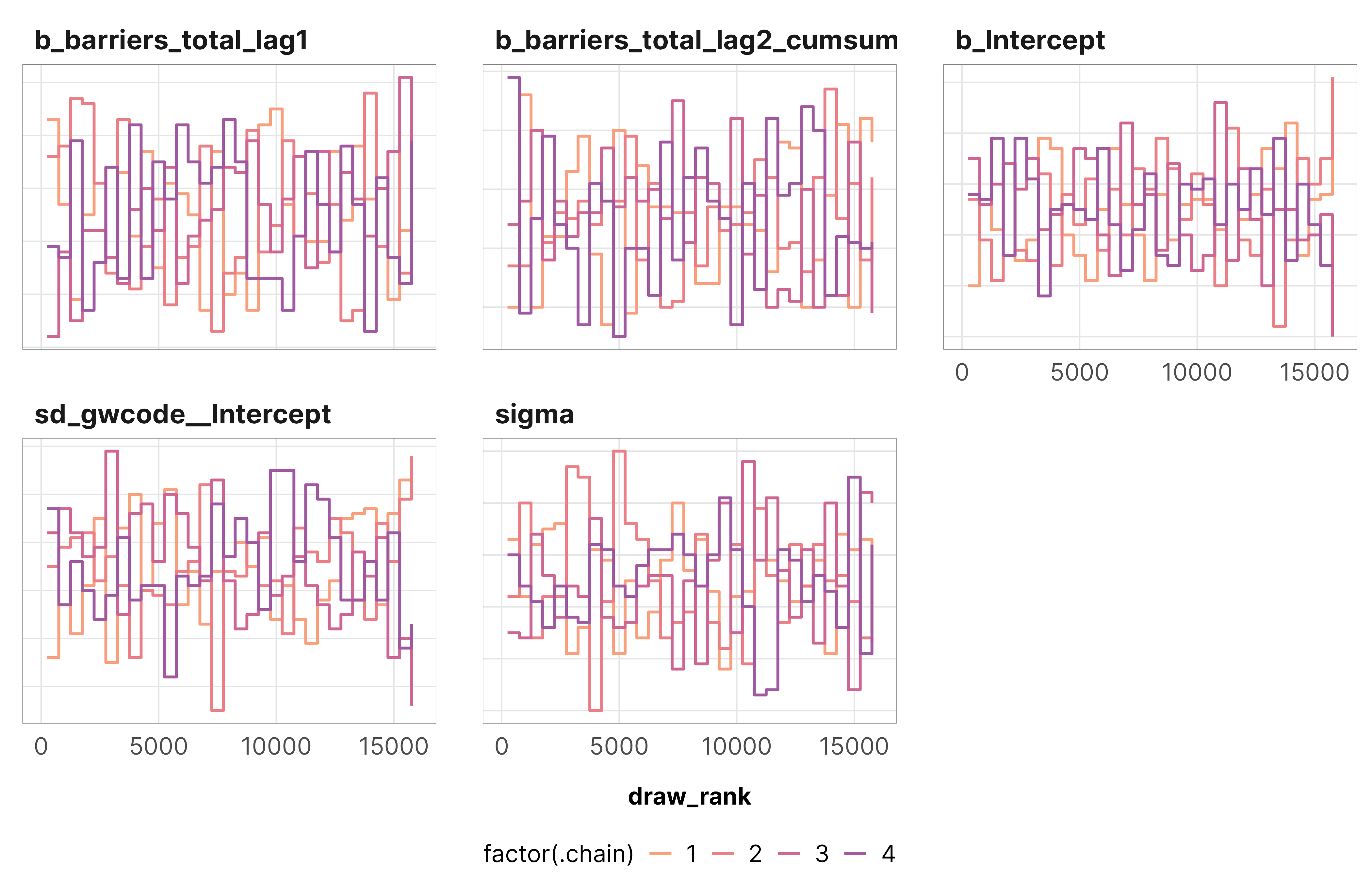
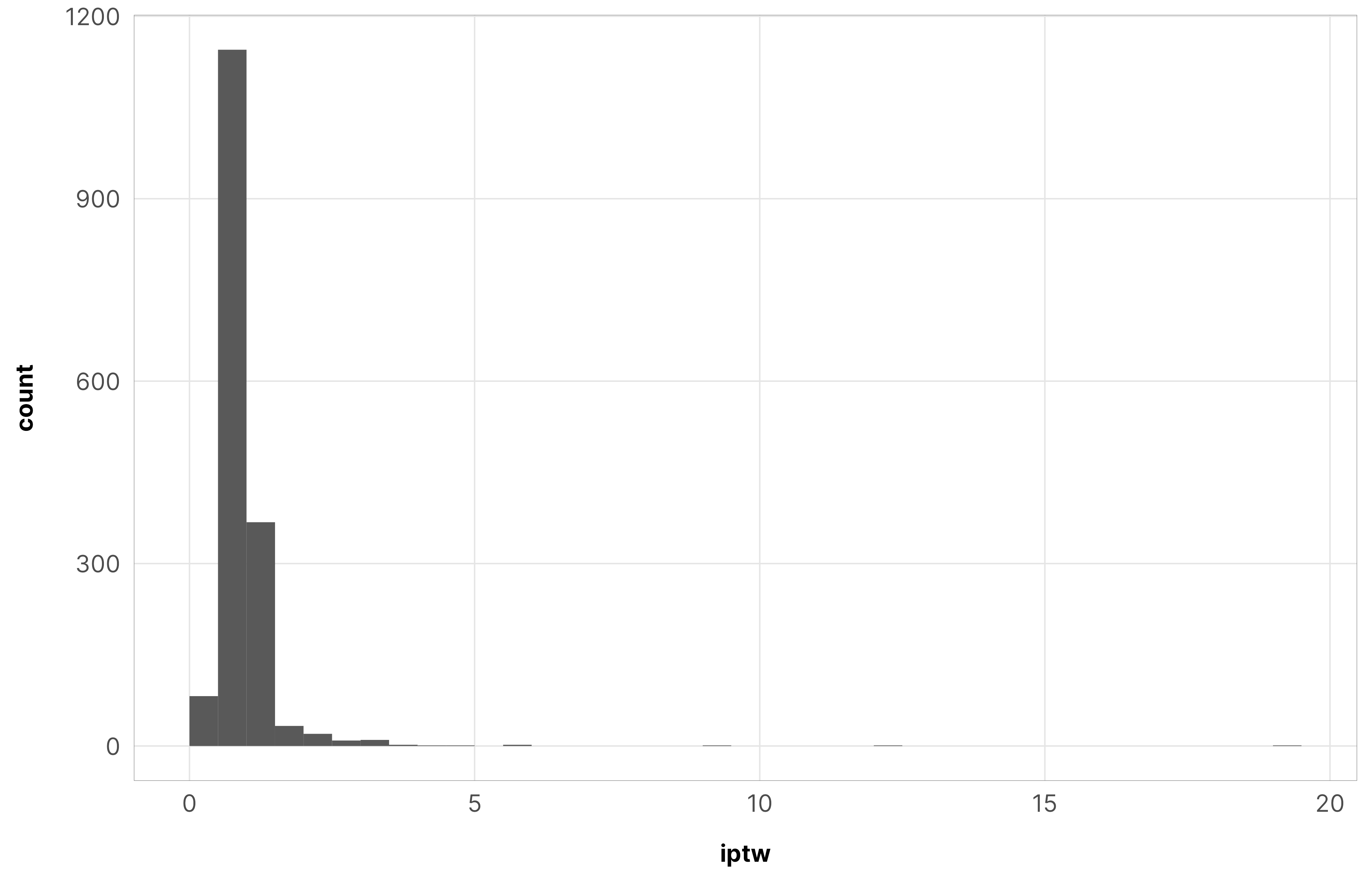
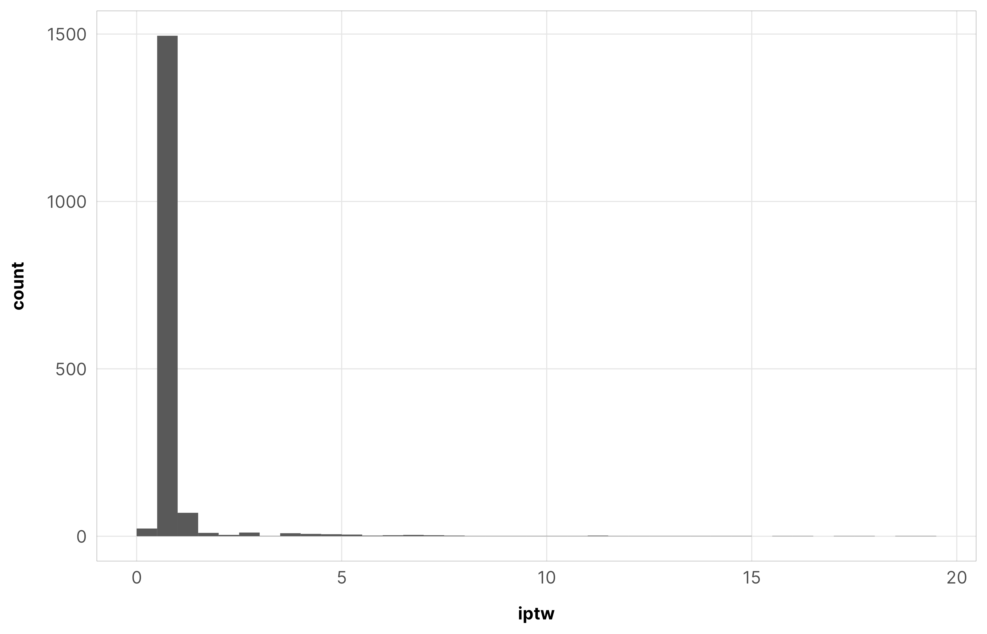
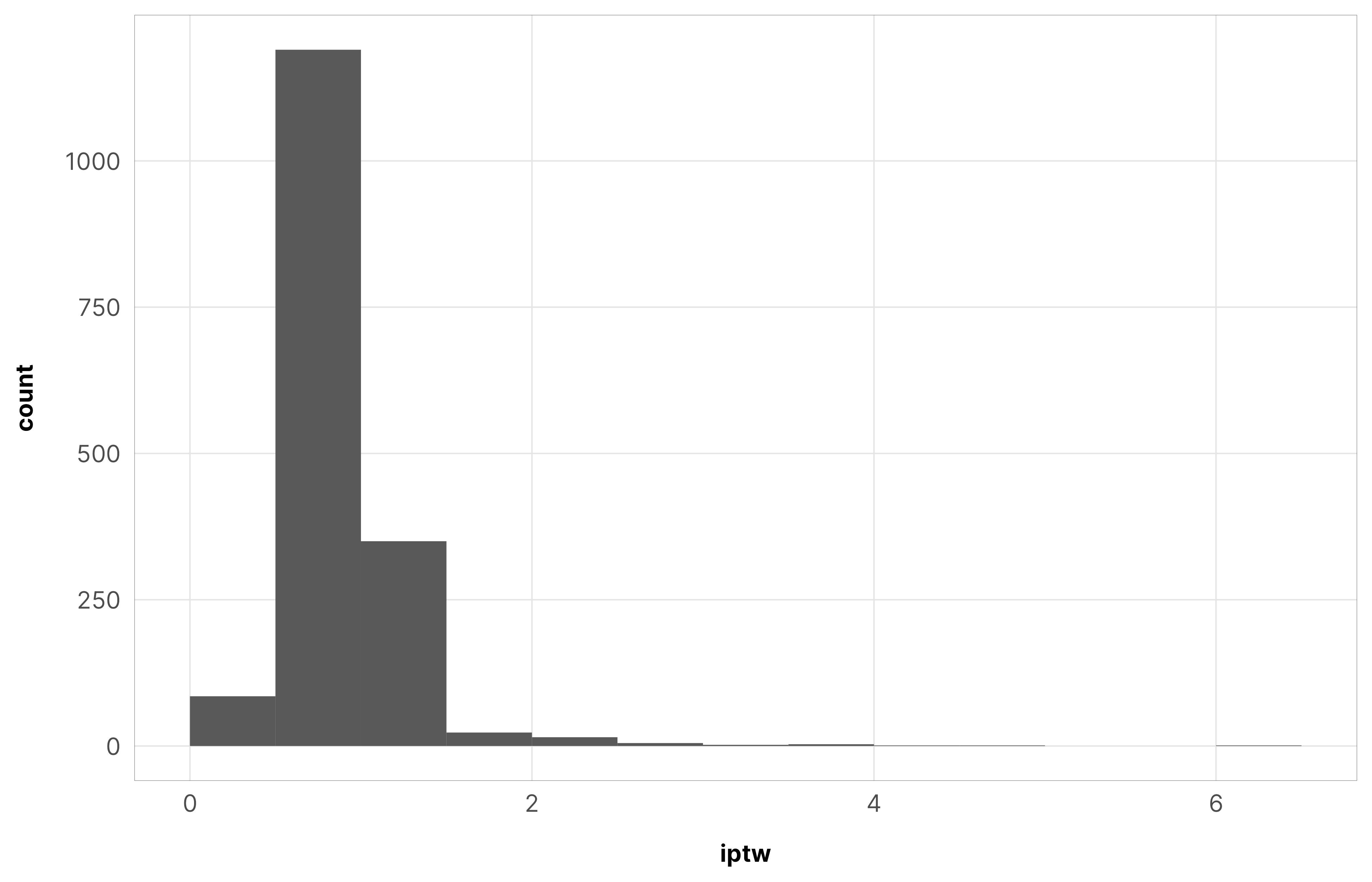
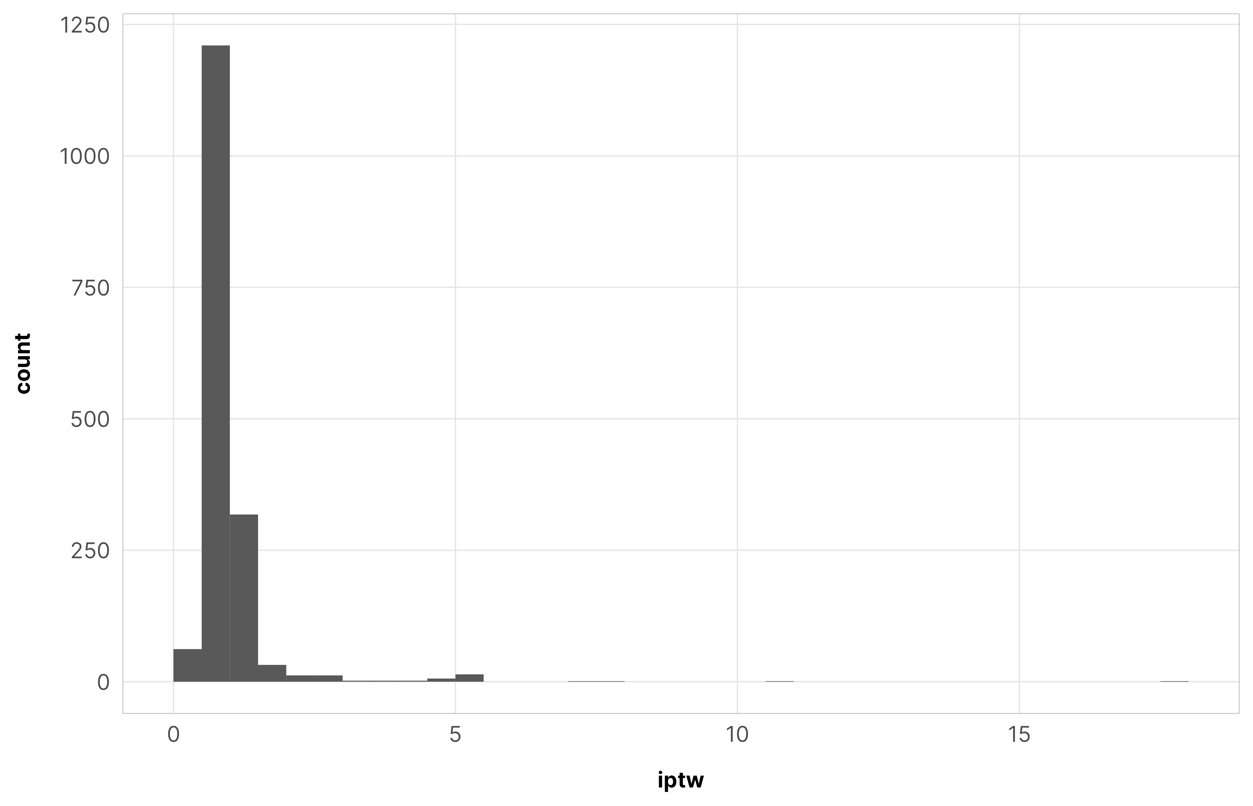
Once again, we verify that everything converged by checking diagnostics for the weight models for the total barriers treatment for domestic NGO recipients. All the other models look basically the same as this—everything is once again fine.

Numerator

Code

m_recip_treatment_total_dom$model_num %>% 
  gather_draws(`^b_.*|^sd_.*|^sigma`, regex = TRUE) %>% 
  ggplot(aes(x = .iteration, y = .value, color = factor(.chain))) +
  geom_line(linewidth = 0.1) +
  scale_color_manual(values = clrs$Sunset[3:6]) +
  facet_wrap(vars(.variable), scales = "free_y") +
  theme_donors()

Code

m_recip_treatment_total_dom$model_num %>% 
  gather_draws(`^b_.*|^sd_.*|^sigma`, regex = TRUE) %>% 
  group_by(.variable) %>% 
  mutate(draw_rank = rank(.value)) %>% 
  ggplot(aes(x = draw_rank, color = factor(.chain))) +
  stat_bin(geom = "step", binwidth = 500, position = position_identity(), boundary = 0) +
  scale_color_manual(values = clrs$Sunset[3:6]) +
  facet_wrap(vars(.variable), scales = "free_y") +
  theme_donors() +
  theme(axis.text.y = element_blank(), axis.title.y = element_blank(), axis.ticks.y = element_blank())

Code

withr::with_seed(1234, {
  pp_check(m_recip_treatment_total_dom$model_num, ndraws = 20) +
    labs(x = "Total NGO barriers",
         title = "Numerator model") +
    theme_donors()
})

Denominator

Code

m_recip_treatment_total_dom$model_denom %>% 
  gather_draws(`^b_.*|^sd_.*|^cor_.*|^sigma`, regex = TRUE) %>% 
  ggplot(aes(x = .iteration, y = .value, color = factor(.chain))) +
  geom_line(linewidth = 0.1) +
  scale_color_manual(values = clrs$Sunset[3:6]) +
  facet_wrap(vars(.variable), scales = "free_y") +
  theme_donors()

Code

m_recip_treatment_total_dom$model_denom %>% 
  gather_draws(`^b_.*|^sd_.*|^cor_.*|^sigma`, regex = TRUE) %>% 
  group_by(.variable) %>% 
  mutate(draw_rank = rank(.value)) %>% 
  ggplot(aes(x = draw_rank, color = factor(.chain))) +
  stat_bin(geom = "step", binwidth = 500, position = position_identity(), boundary = 0) +
  scale_color_manual(values = clrs$Sunset[3:6]) +
  facet_wrap(vars(.variable), scales = "free_y") +
  theme_donors() +
  theme(axis.text.y = element_blank(), axis.title.y = element_blank(), axis.ticks.y = element_blank())

Code

withr::with_seed(1234, {
  pp_check(m_recip_treatment_total_dom$model_denom, ndraws = 20) +
    labs(x = "Total NGO barriers",
         title = "Denominator model") +
    theme_donors()
})

Check weights

As always, IPTWs should generally have a mean of 1 and shouldn’t be too incredibly high.

% of aid to domestic NGO recipients
% of aid to foreign NGO recipients

The max weight here is 19, but once again only a few observations have weights that high. The average is 0.99 and the median is 0.92, which are both essentially 1. Lovely.

Code

summary(df_recip_iptw_total_dom$iptw)
##    Min. 1st Qu.  Median    Mean 3rd Qu.    Max. 
##    0.05    0.81    0.92    0.99    1.01   19.23

Code

df_recip_iptw_total_dom %>% 
  ggplot(aes(x = iptw)) +
  geom_histogram(binwidth = 0.5, boundary = 0) +
  theme_donors()

Same here. The max weight is 20, with an average of 0.99 and a median of 0.92, which are both essentially 1, so we’re still good.

Code

summary(df_recip_iptw_total_foreign$iptw)
##    Min. 1st Qu.  Median    Mean 3rd Qu.    Max. 
##    0.04    0.81    0.92    0.99    1.01   19.61

Code

df_recip_iptw_total_foreign %>% 
  ggplot(aes(x = iptw)) +
  geom_histogram(binwidth = 0.5, boundary = 0) +
  theme_donors()

% of aid to domestic NGO recipients
% of aid to foreign NGO recipients

The max weight here is 19 which is lovely. The average is 1.05, so we’re good.

Code

summary(df_recip_iptw_advocacy_dom$iptw)
##    Min. 1st Qu.  Median    Mean 3rd Qu.    Max. 
##    0.01    0.65    0.78    1.05    0.90   19.27

Code

df_recip_iptw_advocacy_dom %>% 
  ggplot(aes(x = iptw)) +
  geom_histogram(binwidth = 0.5, boundary = 0) +
  theme_donors()

The max weight here is 18 and the average is 1.04, so we’re good.

Code

summary(df_recip_iptw_advocacy_foreign$iptw)
##    Min. 1st Qu.  Median    Mean 3rd Qu.    Max. 
##    0.01    0.65    0.78    1.04    0.90   18.23

Code

df_recip_iptw_advocacy_foreign %>% 
  ggplot(aes(x = iptw)) +
  geom_histogram(binwidth = 0.5, boundary = 0) +
  theme_donors()

% of aid to domestic NGO recipients
% of aid to foreign NGO recipients

The max weight here is 6 which is grand. The average is 0.93, so we’re once again good.

Code

summary(df_recip_iptw_entry_dom$iptw)
##    Min. 1st Qu.  Median    Mean 3rd Qu.    Max. 
##    0.15    0.80    0.91    0.93    1.00    6.15

Code

df_recip_iptw_entry_dom %>% 
  ggplot(aes(x = iptw)) +
  geom_histogram(binwidth = 0.5, boundary = 0) +
  theme_donors()

The max weight here is 6and the average is 0.93. Yay.

Code

summary(df_recip_iptw_entry_foreign$iptw)
##    Min. 1st Qu.  Median    Mean 3rd Qu.    Max. 
##    0.14    0.79    0.90    0.93    0.99    5.79

Code

df_recip_iptw_entry_foreign %>% 
  ggplot(aes(x = iptw)) +
  geom_histogram(binwidth = 0.5, boundary = 0) +
  theme_donors()

% of aid to domestic NGO recipients
% of aid to foreign NGO recipients

The max weight is 18 which is fine, and the average is 1.02, so all is well.

Code

summary(df_recip_iptw_funding_dom$iptw)
##    Min. 1st Qu.  Median    Mean 3rd Qu.    Max. 
##    0.01    0.82    0.92    1.02    1.00   17.98

Code

df_recip_iptw_funding_dom %>% 
  ggplot(aes(x = iptw)) +
  geom_histogram(binwidth = 0.5, boundary = 0) +
  theme_donors()

The max weight here is 20 with an average of 1.02, so all is still well.

Code

summary(df_recip_iptw_funding_foreign$iptw)
##    Min. 1st Qu.  Median    Mean 3rd Qu.    Max. 
##    0.01    0.82    0.92    1.02    0.99   19.98

Code

df_recip_iptw_funding_foreign %>% 
  ggplot(aes(x = iptw)) +
  geom_histogram(binwidth = 0.5, boundary = 0) +
  theme_donors()

% of aid to domestic NGO recipients
% of aid to foreign NGO recipients

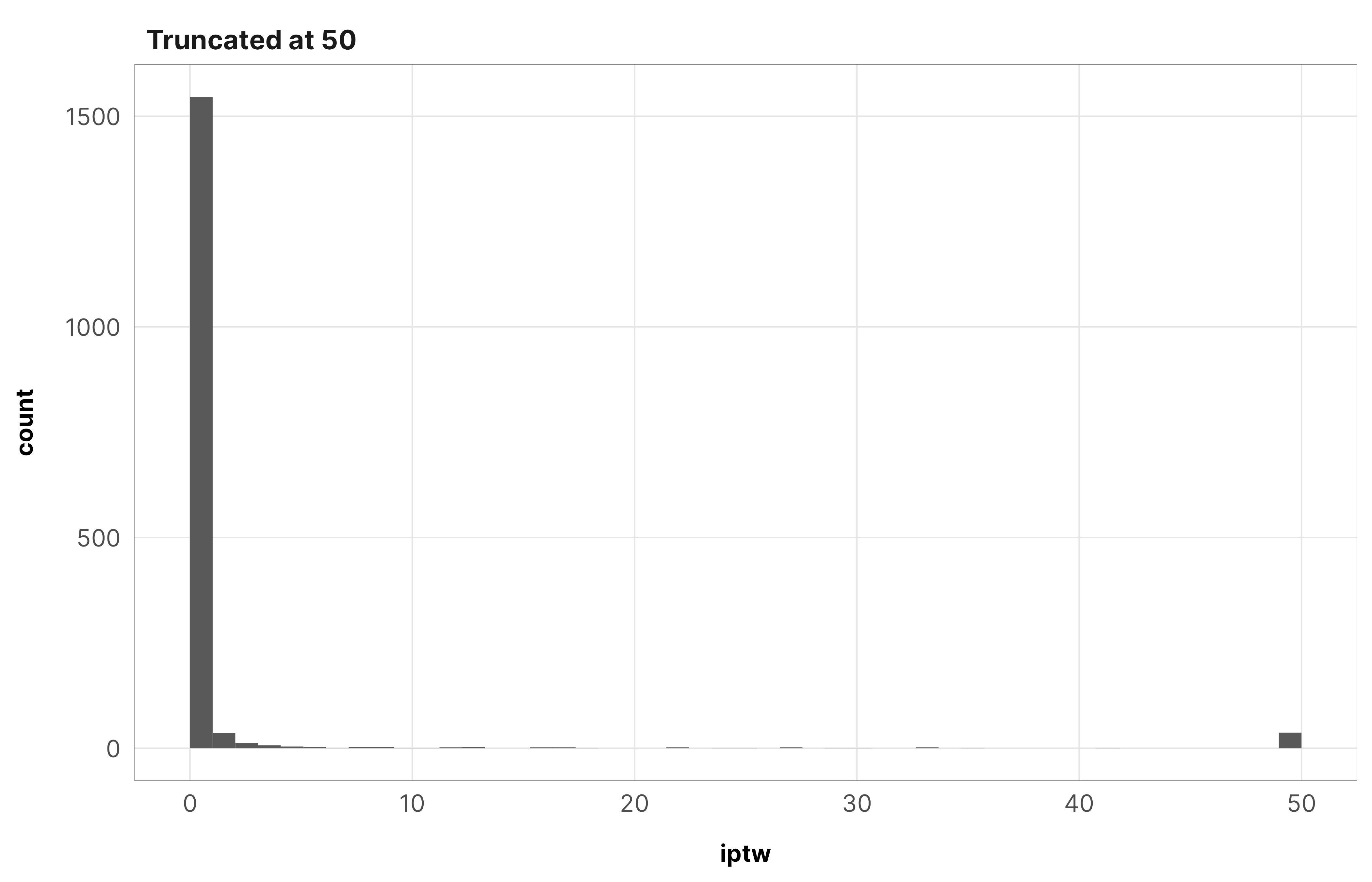
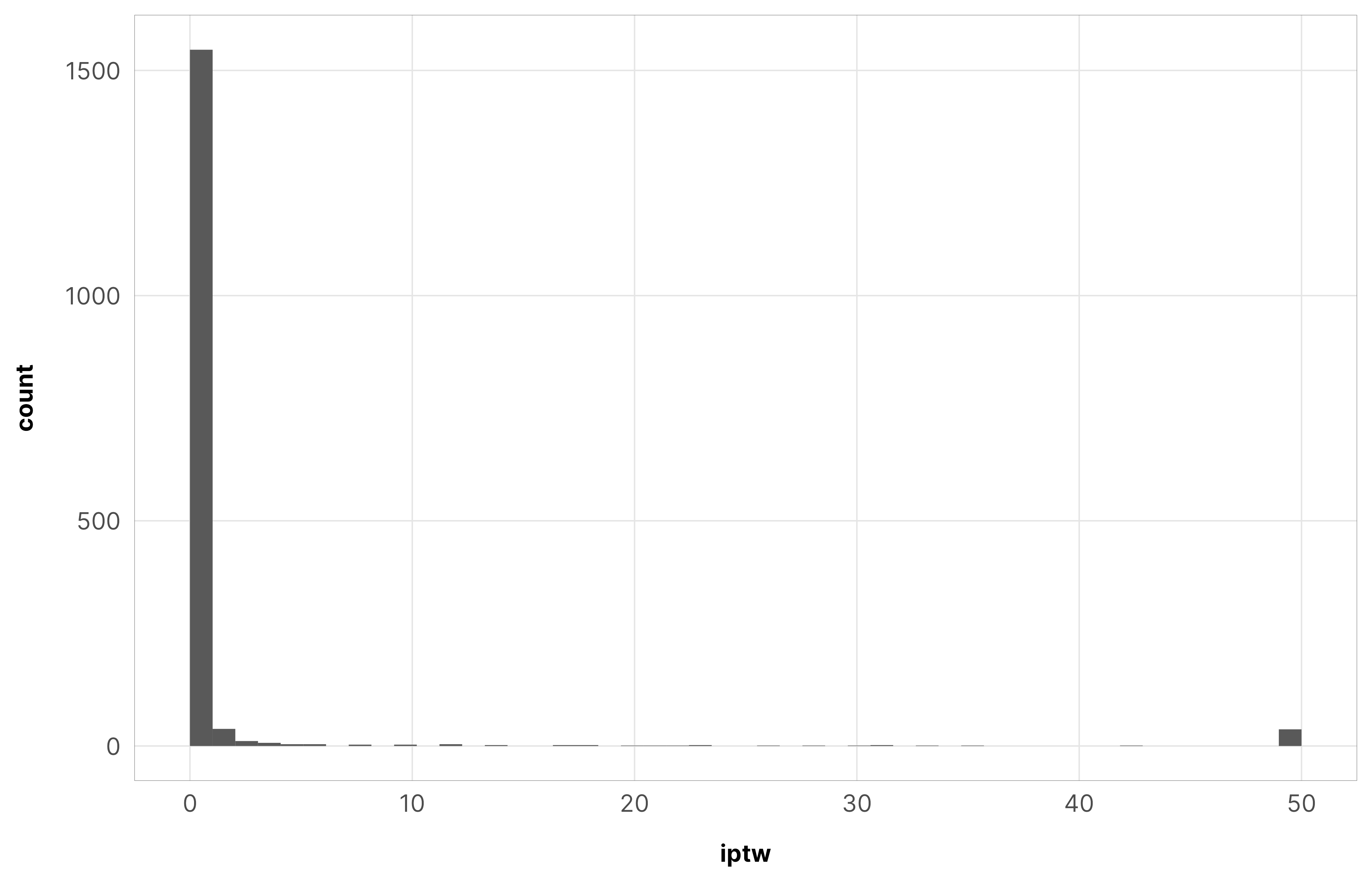
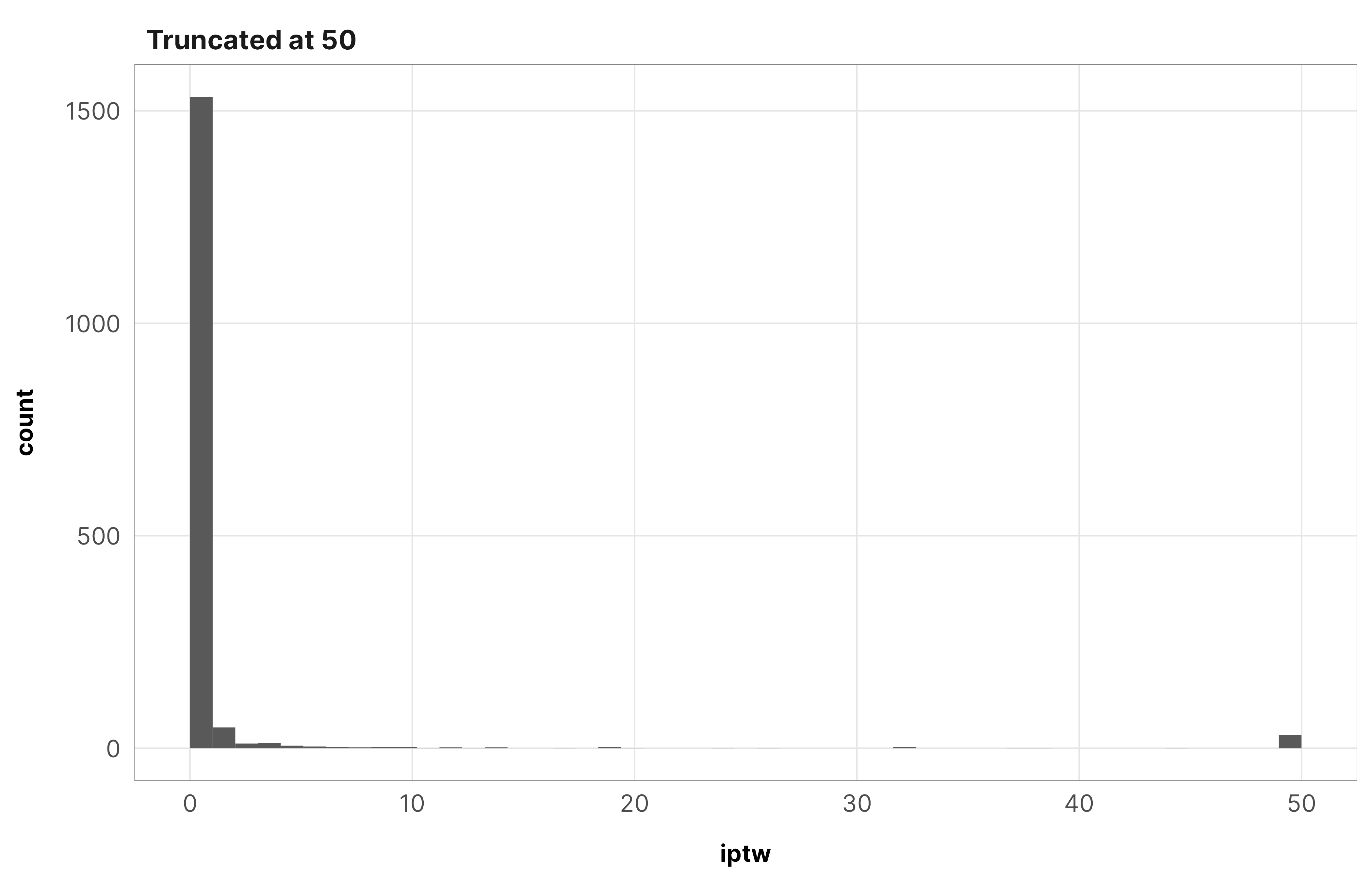
lol, as with the other hypotheses, these once again blow up. The max weight is 19,178,015,127,580.

Code

summary(df_recip_iptw_ccsi_dom$iptw)
##     Min.  1st Qu.   Median     Mean  3rd Qu.     Max. 
## 0.00e+00 0.00e+00 0.00e+00 1.20e+10 0.00e+00 1.92e+13

There aren’t a lot of observations with weights that high though. Check out the counts of rows with weights greater than 50 and greater than 500—only 100ish:

Code

df_recip_iptw_ccsi_dom %>% count(iptw >= 50)
## # A tibble: 2 × 2
##   `iptw >= 50`     n
##   <lgl>        <int>
## 1 FALSE         1639
## 2 TRUE            37
df_recip_iptw_ccsi_dom %>% count(iptw >= 500)
## # A tibble: 2 × 2
##   `iptw >= 500`     n
##   <lgl>         <int>
## 1 FALSE          1652
## 2 TRUE             24

We truncate these weights at 50.

Code

plot_iptw_ccsi_dom <- bind_rows(
  df_recip_iptw_ccsi_dom %>% mutate(threshold = 50, iptw = ifelse(iptw > threshold, threshold, iptw)),
  df_recip_iptw_ccsi_dom %>% mutate(threshold = 500, iptw = ifelse(iptw > threshold, threshold, iptw))
) %>% 
  mutate(threshold = paste0("Truncated at ", threshold),
         threshold = fct_inorder(threshold))

plot_iptw_ccsi_dom %>% 
  ggplot(aes(x = iptw)) +
  geom_histogram(bins = 50, boundary = 0) +
  facet_wrap(vars(threshold), scales = "free_x") +
  theme_donors()

Same here—these blow up in a comically huge way.

Code

summary(df_recip_iptw_ccsi_foreign$iptw)
##     Min.  1st Qu.   Median     Mean  3rd Qu.     Max. 
## 0.00e+00 0.00e+00 0.00e+00 1.57e+10 0.00e+00 2.52e+13

We also truncate these weights at 50.

Code

plot_iptw_ccsi_foreign <- df_recip_iptw_ccsi_foreign %>% 
  mutate(threshold = 50, iptw = ifelse(iptw > threshold, threshold, iptw)) %>% 
  mutate(threshold = paste0("Truncated at ", threshold),
         threshold = fct_inorder(threshold))

plot_iptw_ccsi_foreign %>% 
  ggplot(aes(x = iptw)) +
  geom_histogram(bins = 50, boundary = 0) +
  facet_wrap(vars(threshold), scales = "free_x") +
  theme_donors()

% of aid to domestic NGO recipients
% of aid to foreign NGO recipients

These weights are also horrendous, with a maximum weight of 5,256,086,475.

Code

summary(df_recip_iptw_repress_dom$iptw)
##     Min.  1st Qu.   Median     Mean  3rd Qu.     Max. 
## 0.00e+00 0.00e+00 0.00e+00 3.14e+06 0.00e+00 5.26e+09

As with the core civil society index, there aren’t a lot of observations with weights that high:

Code

df_recip_iptw_repress_dom %>% count(iptw >= 50)
## # A tibble: 2 × 2
##   `iptw >= 50`     n
##   <lgl>        <int>
## 1 FALSE         1645
## 2 TRUE            31
df_recip_iptw_repress_dom %>% count(iptw >= 500)
## # A tibble: 2 × 2
##   `iptw >= 500`     n
##   <lgl>         <int>
## 1 FALSE          1663
## 2 TRUE             13

So we truncate these weights at 50 again. Since the results from the core civil society models are basically the same when truncating at 500, we only use a truncation point of 50 here.

Code

df_recip_iptw_ccsi_dom %>% 
  mutate(threshold = 50, iptw = ifelse(iptw > threshold, threshold, iptw)) %>% 
  ggplot(aes(x = iptw)) +
  geom_histogram(bins = 50, boundary = 0) +
  theme_donors()

Once again, lolz.

Code

summary(df_recip_iptw_repress_foreign$iptw)
##     Min.  1st Qu.   Median     Mean  3rd Qu.     Max. 
## 0.00e+00 0.00e+00 0.00e+00 3.05e+06 0.00e+00 5.10e+09

We also truncate these weights at 50.

Code

plot_iptw_repress_foreign <- df_recip_iptw_repress_foreign %>% 
  mutate(threshold = 50, iptw = ifelse(iptw > threshold, threshold, iptw)) %>% 
  mutate(threshold = paste0("Truncated at ", threshold),
         threshold = fct_inorder(threshold))

plot_iptw_repress_foreign %>% 
  ggplot(aes(x = iptw)) +
  geom_histogram(bins = 50, boundary = 0) +
  facet_wrap(vars(threshold), scales = "free_x") +
  theme_donors()

Results

These are less important since we just use these treatment models to generate weights and because interpreting each coefficient when trying to isolate causal effects is unimportant (Westreich and Greenland 2013; Keele, Stevenson, and Elwert 2020).

% of aid to domestic NGO recipients
% of aid to foreign NGO recipients

Numerator
Denominator

Code

models_tbl_h3_treatment_num_dom <- models_tbl_h3_treatment_num_dom %>% 
  set_names(1:length(.))

notes <- c(
  "Posterior medians; 95% credible intervals in brackets", 
  "Total \\(R^2\\) considers the variance of both population and group effects", 
  "Marginal \\(R^2\\) only takes population effects into account"
)

modelsummary(models_tbl_h3_treatment_num_dom,
             estimate = "{estimate}",
             statistic = "[{conf.low}, {conf.high}]",
             add_rows = treatment_rows,
             coef_map = coefs_num,
             gof_map = gofs,
             output = "kableExtra",
             fmt =  list(estimate = 2, conf.low = 2, conf.high = 2)) %>% 
  row_spec(1, bold = TRUE) %>% 
  kable_styling(htmltable_class = "table-sm light-border")

?(caption)

Code

models_tbl_h3_treatment_denom_dom <- models_tbl_h3_treatment_denom_dom %>% 
  set_names(1:length(.))

notes <- c(
  "Posterior medians; 95% credible intervals in brackets", 
  "Total \\(R^2\\) considers the variance of both population and group effects", 
  "Marginal \\(R^2\\) only takes population effects into account"
)

modelsummary(models_tbl_h3_treatment_denom_dom,
             estimate = "{estimate}",
             statistic = "[{conf.low}, {conf.high}]",
             add_rows = treatment_rows,
             coef_map = coefs_denom,
             gof_map = gofs,
             fmt =  list(estimate = 2, conf.low = 2, conf.high = 2),
             notes = notes) %>% 
  row_spec(1, bold = TRUE) %>% 
  kable_styling(htmltable_class = "table-sm light-border")

?(caption)

Numerator
Denominator

Code

models_tbl_h3_treatment_num_foreign <- models_tbl_h3_treatment_num_foreign %>% 
  set_names(1:length(.))

notes <- c(
  "Posterior medians; 95% credible intervals in brackets", 
  "Total \\(R^2\\) considers the variance of both population and group effects", 
  "Marginal \\(R^2\\) only takes population effects into account"
)

modelsummary(models_tbl_h3_treatment_num_foreign,
             estimate = "{estimate}",
             statistic = "[{conf.low}, {conf.high}]",
             add_rows = treatment_rows,
             coef_map = coefs_num,
             gof_map = gofs,
             output = "kableExtra",
             fmt =  list(estimate = 2, conf.low = 2, conf.high = 2)) %>% 
  row_spec(1, bold = TRUE) %>% 
  kable_styling(htmltable_class = "table-sm light-border")

?(caption)

Code

models_tbl_h3_treatment_denom_foreign <- models_tbl_h3_treatment_denom_foreign %>% 
  set_names(1:length(.))

notes <- c(
  "Posterior medians; 95% credible intervals in brackets", 
  "Total \\(R^2\\) considers the variance of both population and group effects", 
  "Marginal \\(R^2\\) only takes population effects into account"
)

modelsummary(models_tbl_h3_treatment_denom_foreign,
             estimate = "{estimate}",
             statistic = "[{conf.low}, {conf.high}]",
             add_rows = treatment_rows,
             coef_map = coefs_denom,
             gof_map = gofs,
             fmt =  list(estimate = 2, conf.low = 2, conf.high = 2),
             notes = notes) %>% 
  row_spec(1, bold = TRUE) %>% 
  kable_styling(htmltable_class = "table-sm light-border")

?(caption)

Outcome models

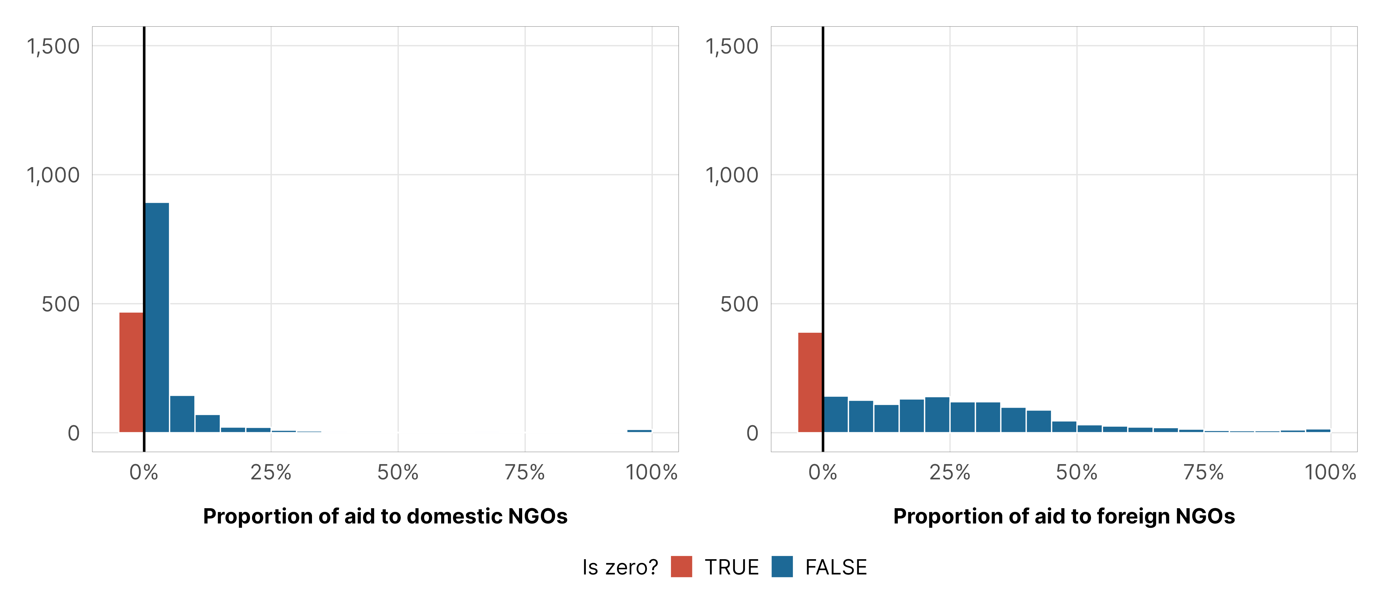
Our outcome variable for these hypotheses is the proportion of USAID aid allocated to (1) domestic and (2) foreign NGOs, which are (1) bounded between 0% and 100% and (2) have a lot of zeros.

Code

bind_rows(
  `Proportion of aid to domestic NGOs` = count(df_country_aid_laws, is_zero = prop_ngo_dom == 0),
  `Proportion of aid to foreign NGOs` = count(df_country_aid_laws, is_zero = prop_ngo_foreign == 0),
  .id = "Outcome"
) %>% 
  group_by(Outcome) %>% 
  mutate(`Number of 0s` = glue::glue("{n[2]} / {sum(n)}")) %>% 
  mutate(`Proportion of 0s` = label_percent(accuracy = 0.1)(n / sum(n))) %>% 
  ungroup() %>% 
  filter(is_zero) %>% select(-is_zero, -n) %>% 
  kbl(align = c("l", "c", "c")) %>% 
  kable_styling(htmltable_class = "table table-sm",
                full_width = FALSE)

Table 1: 0s in recipient outcomes
Outcome	Number of 0s	Proportion of 0s
Proportion of aid to domestic NGOs	468 / 1676	27.9%
Proportion of aid to foreign NGOs	390 / 1676	23.3%

Code

p1 <- df_country_aid_laws %>%
  mutate(is_zero = prop_ngo_dom == 0) %>% 
  mutate(prop_ngo_dom = ifelse(is_zero, -0.05, prop_ngo_dom))  %>%  
  ggplot(aes(x = prop_ngo_dom)) +
  geom_histogram(aes(fill = is_zero), binwidth = 0.05, 
                 linewidth = 0.25, boundary = 0, color = "white") +
  geom_vline(xintercept = 0) + 
  scale_x_continuous(labels = label_percent()) +
  scale_y_continuous(labels = label_comma()) +
  scale_fill_manual(values = c(clrs$Prism[2], clrs$Prism[8]), 
                    guide = guide_legend(reverse = TRUE)) +
  labs(x = "Proportion of aid to domestic NGOs", y = NULL, fill = "Is zero?") +
  coord_cartesian(ylim = c(0, 1500)) +
  theme_donors() +
  theme(legend.position = "bottom")

p2 <- df_country_aid_laws %>%
  mutate(is_zero = prop_ngo_foreign == 0) %>% 
  mutate(prop_ngo_foreign = ifelse(is_zero, -0.05, prop_ngo_foreign))  %>%  
  ggplot(aes(x = prop_ngo_foreign)) +
  geom_histogram(aes(fill = is_zero), binwidth = 0.05, 
                 linewidth = 0.25, boundary = 0, color = "white") +
  geom_vline(xintercept = 0) + 
  scale_x_continuous(labels = label_percent()) +
  scale_y_continuous(labels = label_comma()) +
  scale_fill_manual(values = c(clrs$Prism[2], clrs$Prism[8]), 
                    guide = guide_legend(reverse = TRUE)) +
  labs(x = "Proportion of aid to foreign NGOs", y = NULL, fill = "Is zero?") +
  coord_cartesian(ylim = c(0, 1500)) +
  theme_donors() +
  theme(legend.position = "bottom")

(p1 | p2) +
  plot_layout(guides = "collect") +
  plot_annotation(theme = theme(legend.position = "bottom"))

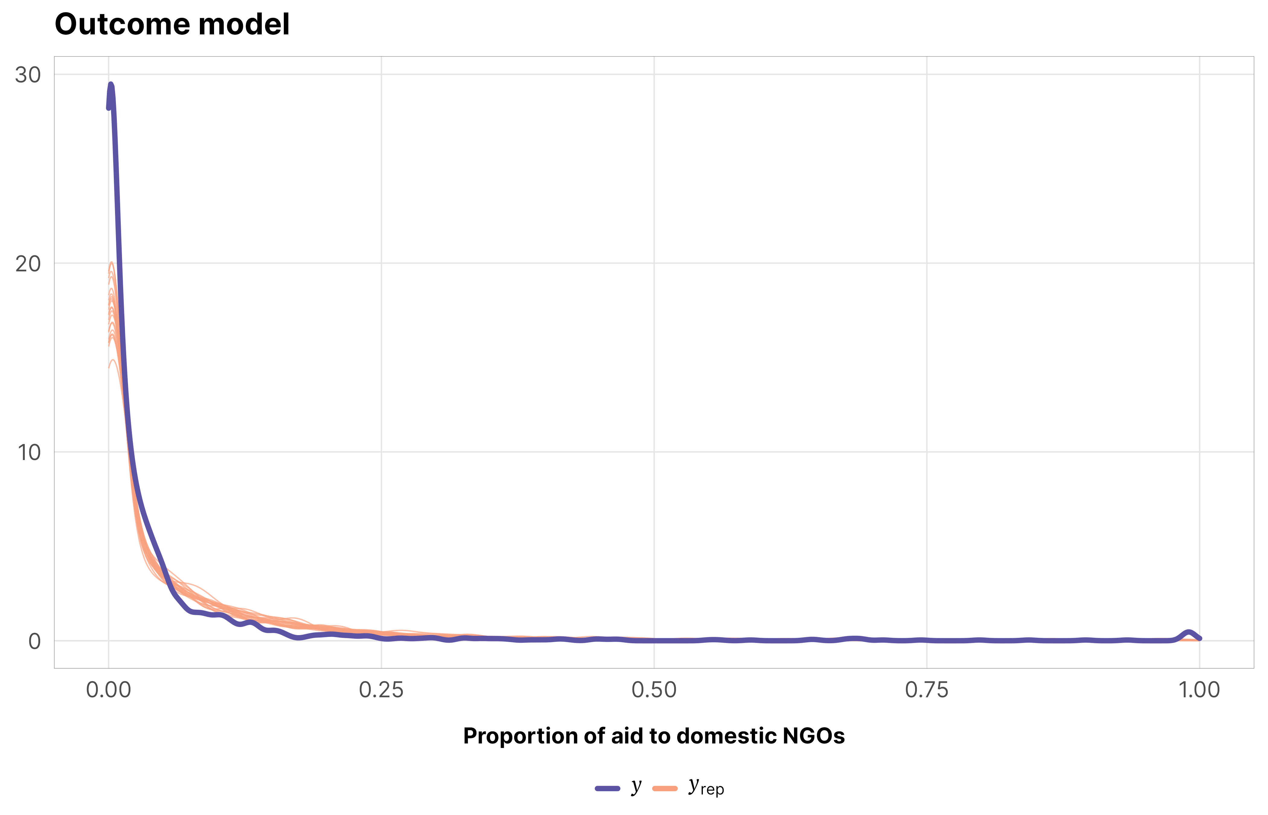
Because of this distribution, we use a zero-inflated beta family to model the outcome. This guide to working with tricky outcomes with lots of zeros explores all the intricacies of zero-inflated beta families, so we won’t go into tons of detail here.

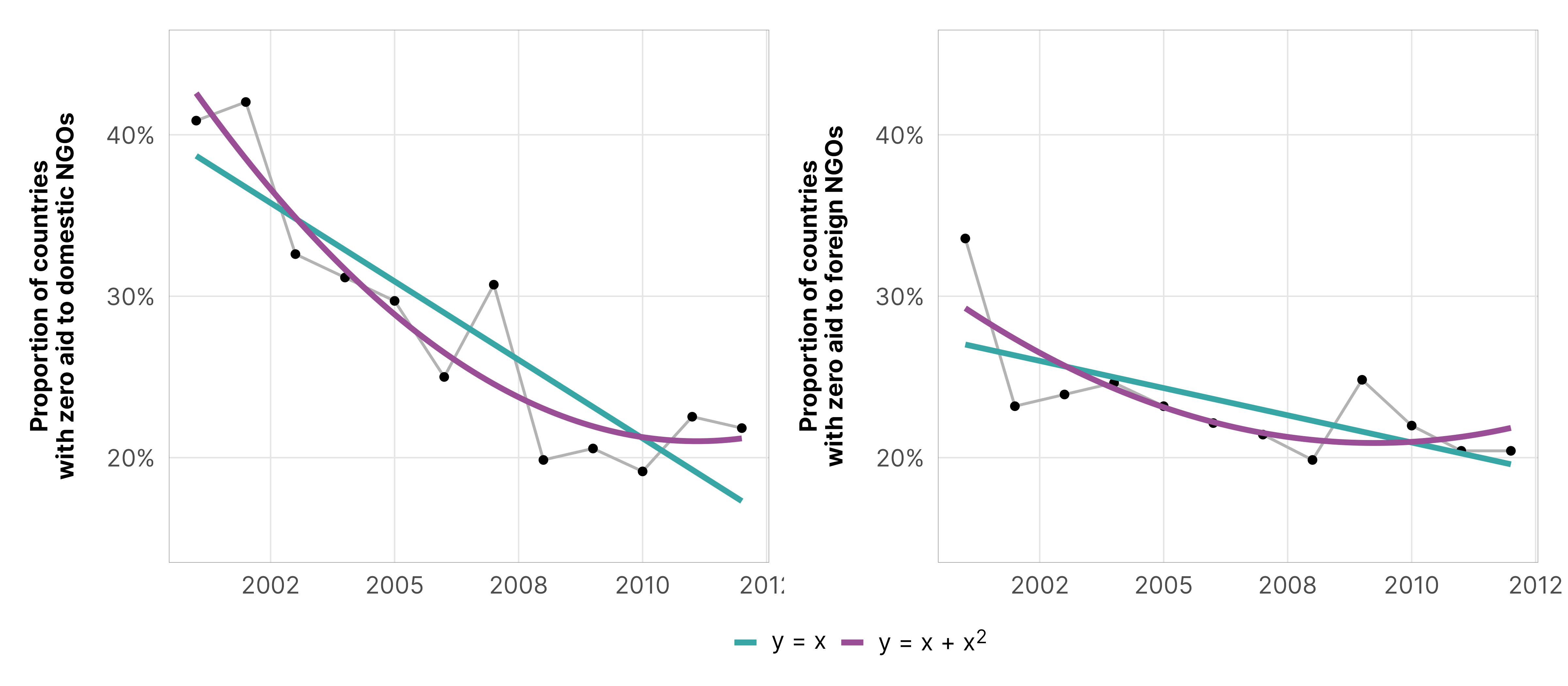
As with total foreign aid and aid contentiousness, we’re not entirely sure what the actual underlying zero process is for the proportion of aid to different recipients. There’s definitely a time-related aspect—aid to both kinds of NGOs decreases over time (replaced with corresponding increases to governments and multilateral organizations like regional development banks). The trend is fairly linear, but to stay consistent with our hurdle and zero-inflated modeling strategies from the previous hypotheses, we still include year squared in the model.

Code

p1 <- df_country_aid_laws %>% 
  group_by(year) %>% 
  summarize(prop_zero = mean(prop_ngo_dom == 0)) %>% 
  ggplot(aes(x = year, y = prop_zero)) +
  geom_line(linewidth = 0.5, color = "grey70") +
  geom_point(size = 1) + 
  geom_smooth(aes(color = "y = x"), method = "lm", 
              formula = y ~ x, se = FALSE) +
  geom_smooth(aes(color = "y = x + x<sup>2</sup>"), method = "lm", 
              formula = y ~ x + I(x^2), se = FALSE) +
  scale_y_continuous(labels = label_percent()) +
  scale_color_manual(values = clrs$Prism[c(3, 11)]) +
  labs(x = NULL, y = "Proportion of countries\nwith zero aid to domestic NGOs",
       color = NULL) +
  coord_cartesian(ylim = c(0.15, 0.45)) +
  theme_donors() +
  theme(legend.text = element_markdown())

p2 <- df_country_aid_laws %>% 
  group_by(year) %>% 
  summarize(prop_zero = mean(prop_ngo_foreign == 0)) %>% 
  ggplot(aes(x = year, y = prop_zero)) +
  geom_line(linewidth = 0.5, color = "grey70") +
  geom_point(size = 1) + 
  geom_smooth(aes(color = "y = x"), method = "lm", 
              formula = y ~ x, se = FALSE) +
  geom_smooth(aes(color = "y = x + x<sup>2</sup>"), method = "lm", 
              formula = y ~ x + I(x^2), se = FALSE) +
  scale_y_continuous(labels = label_percent()) +
  scale_color_manual(values = clrs$Prism[c(3, 11)]) +
  labs(x = NULL, y = "Proportion of countries\nwith zero aid to foreign NGOs",
       color = NULL) +
  coord_cartesian(ylim = c(0.15, 0.45)) +
  theme_donors() +
  theme(legend.text = element_markdown())

(p1 | p2) +
  plot_layout(guides = "collect") +
  plot_annotation(theme = theme(legend.position = "bottom"))

Formal model and priors

Our final models look like this (again with treatment replaced by the actual treatment column):

Domestic NGO recipients
Foreign NGO recipients

Code

bf(prop_ngo_dom | weights(iptw) ~ treatment_lag1 + treatment_lag2_cumsum +
     year_c + (1 + year_c | gwcode),
   zi ~ year_c + I(year_c^2))

Code

bf(prop_ngo_foreign | weights(iptw) ~ treatment_lag1 + treatment_lag2_cumsum +
     year_c + (1 + year_c | gwcode),
   zi ~ year_c + I(year_c^2))

Or more formally:

\[ \begin{aligned} &\ \mathrlap{\textbf{Zero-inflated model of proportion $i$ across time $t$ within each country $j$}} \\ \text{Proportion}_{it_j} \sim&\ \mathrlap{\begin{cases} 0 & \text{with probability } \pi_{it} + [(1 - \pi_{it}) \times \operatorname{Beta}(0 \mid \mu_{it_j}, \phi_y)] \\[4pt] \operatorname{Beta}(\mu_{it_j}, \phi_y) & \text{with probability } (1 - \pi_{it}) \times \operatorname{Beta}(\text{Proportion}_{it_j} \mid \mu_{it_j}, \phi_y) \end{cases}} \\ \\ &\ \textbf{Models for distribution parameters} \\ \operatorname{logit}(\pi_{it}) =&\ \gamma_0 + \gamma_1 \text{Year}_{it} + \gamma_2 \text{Year}^2_{it} & \text{Zero-inflation process} \\[4pt] \operatorname{logit}(\mu_{it_j}) =&\ \text{IPTW}_{i, t-1_j} \times \Bigl[ (\beta_0 + b_{0_j}) + \beta_1\, \text{Treatment}_{i, t-1_j} + \\ &\ \beta_2\, \textstyle{\sum_{\tau = (t-2)}^{t}} \text{Treatment}_{i\tau} + (\beta_3 + b_{3_j}) \text{Year}_{it_j} \Bigr] & \text{Within-country variation} \\[4pt] \left( \begin{array}{c} b_{0_j} \\ b_{3_j} \end{array} \right) \sim&\ \text{MV}\,\mathcal{N} \left[ \left( \begin{array}{c} 0 \\ 0 \\ \end{array} \right) , \, \left( \begin{array}{cc} \sigma^2_{0} & \rho_{0, 3}\, \sigma_{0} \sigma_{3} \\ \cdots & \sigma^2_{3} \end{array} \right) \right] & \text{Variability in average intercepts and slopes} \\ \\ &\ \textbf{Priors} \\ \gamma_0 \sim&\ \text{Student $t$}(\nu = 3, \mu = 0, \sigma = 1.5) & \text{Prior for intercept in zero-inflated model} \\ \gamma_1, \gamma_2 \sim&\ \text{Student $t$}(3, 0, 1.5) & \text{Prior for year effect in zero-inflated model} \\ \beta_0 \sim&\ \text{Student $t$}(3, 0, 1.5) & \text{Prior for global average proportion} \\ \beta_1, \beta_2, \beta_3 \sim&\ \text{Student $t$}(3, 0, 1.5) & \text{Prior for global effects} \\ \phi_y \sim&\ \operatorname{Exponential}(1) & \text{Prior for within-country dispersion} \\ \sigma_0, \sigma_3 \sim&\ \operatorname{Exponential}(1) & \text{Prior for within-country variability} \\ \rho \sim&\ \operatorname{LKJ}(2) & \text{Prior for between-country variability} \end{aligned} \]

MCMC diagnostics

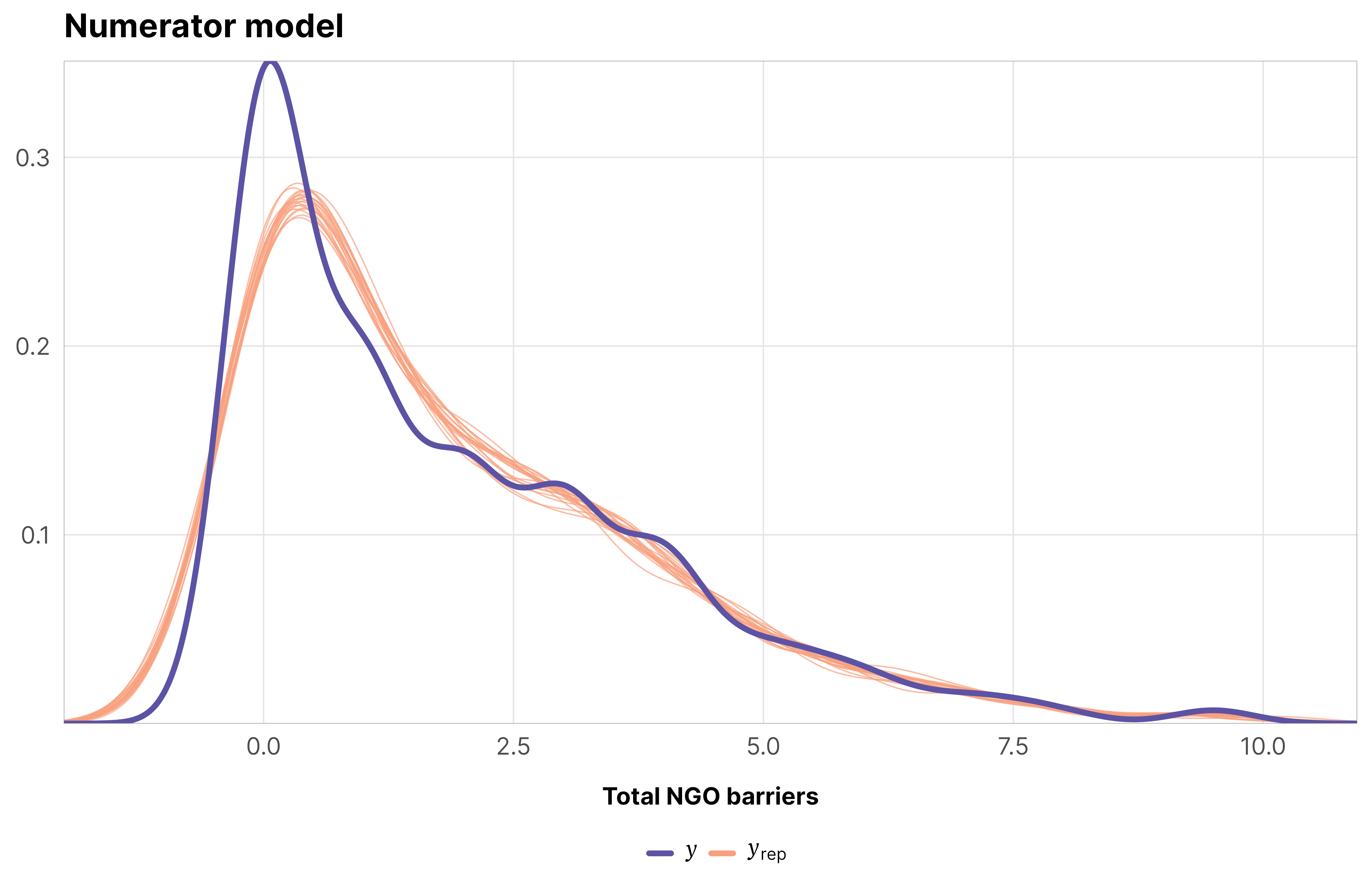
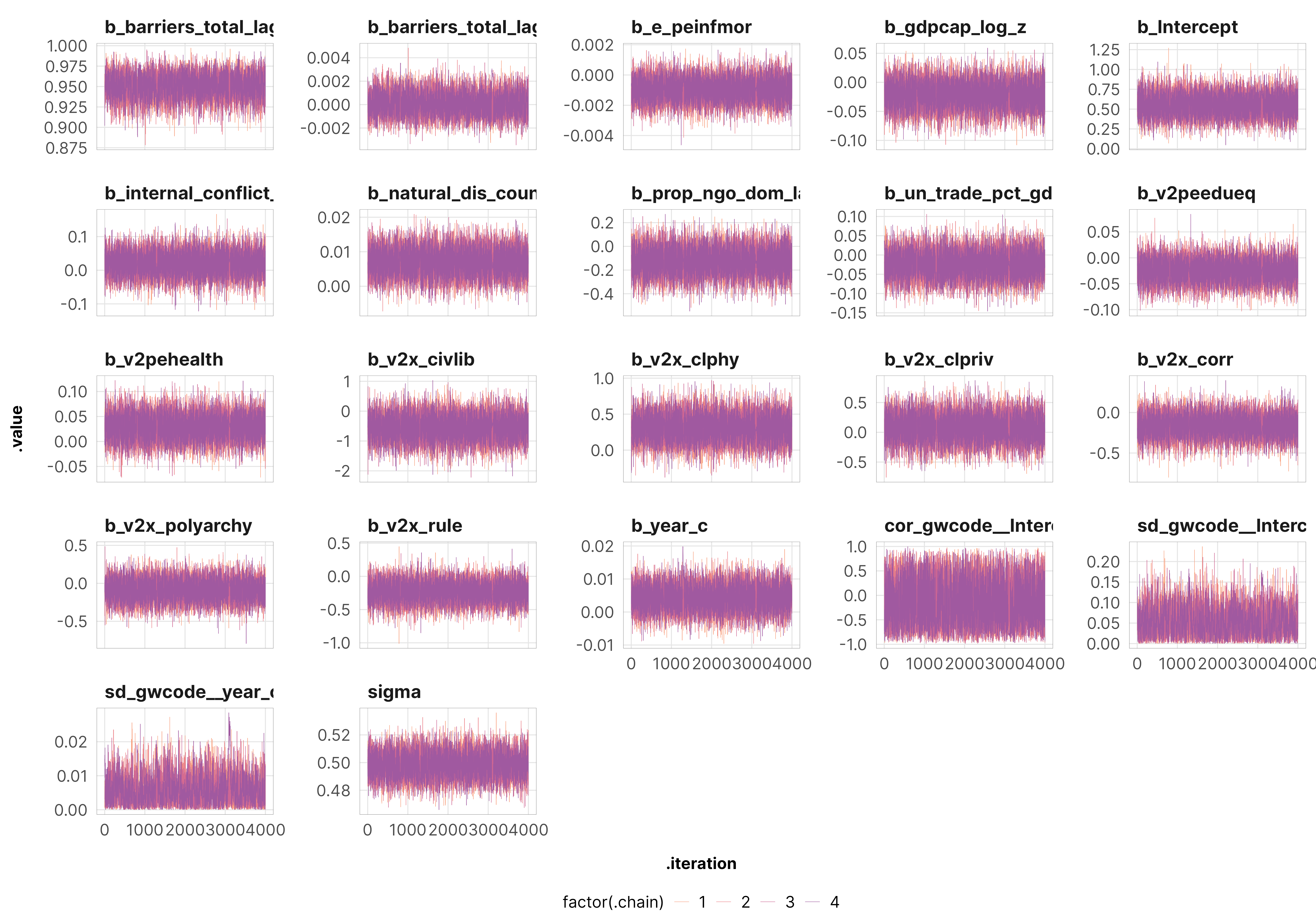
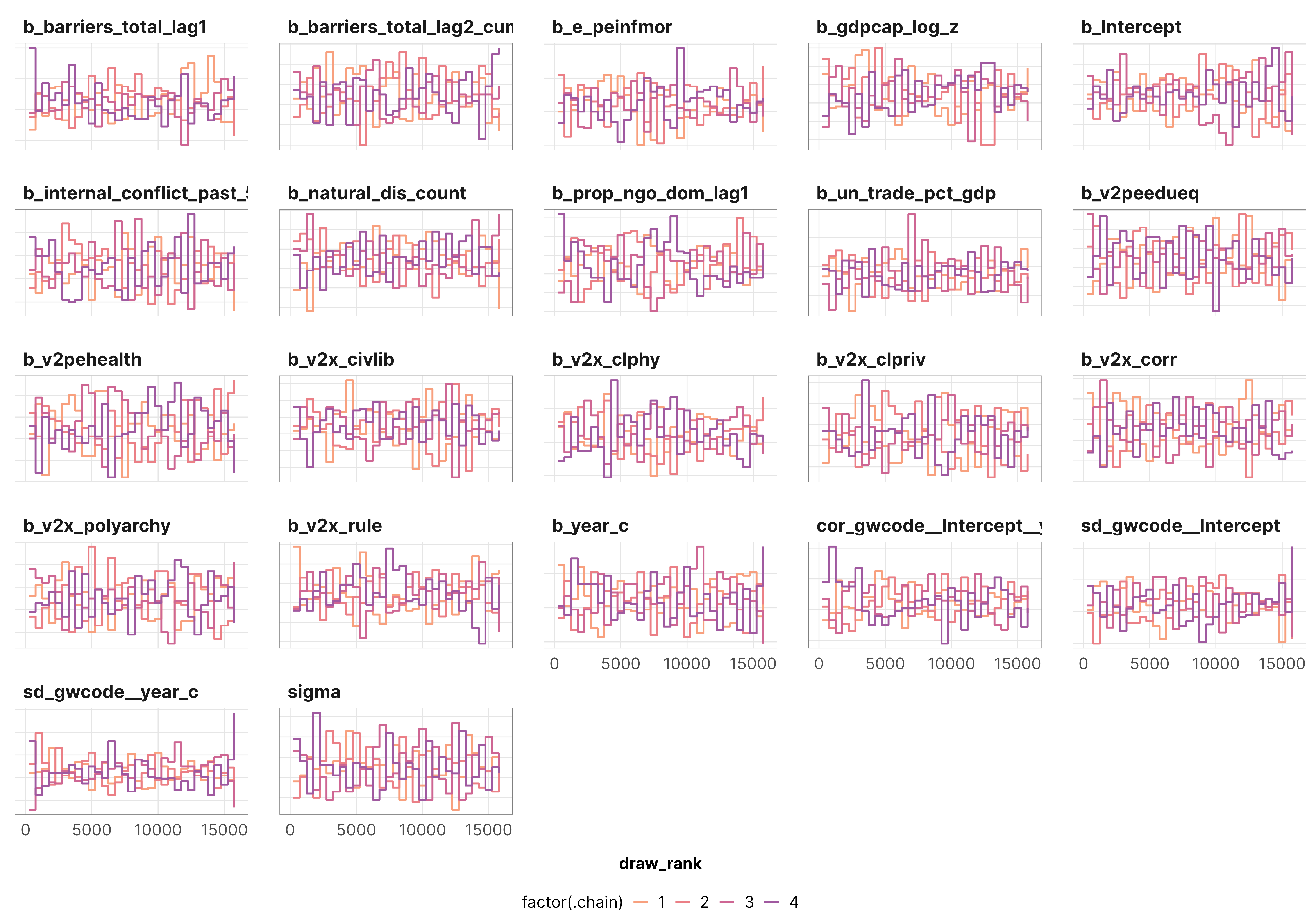
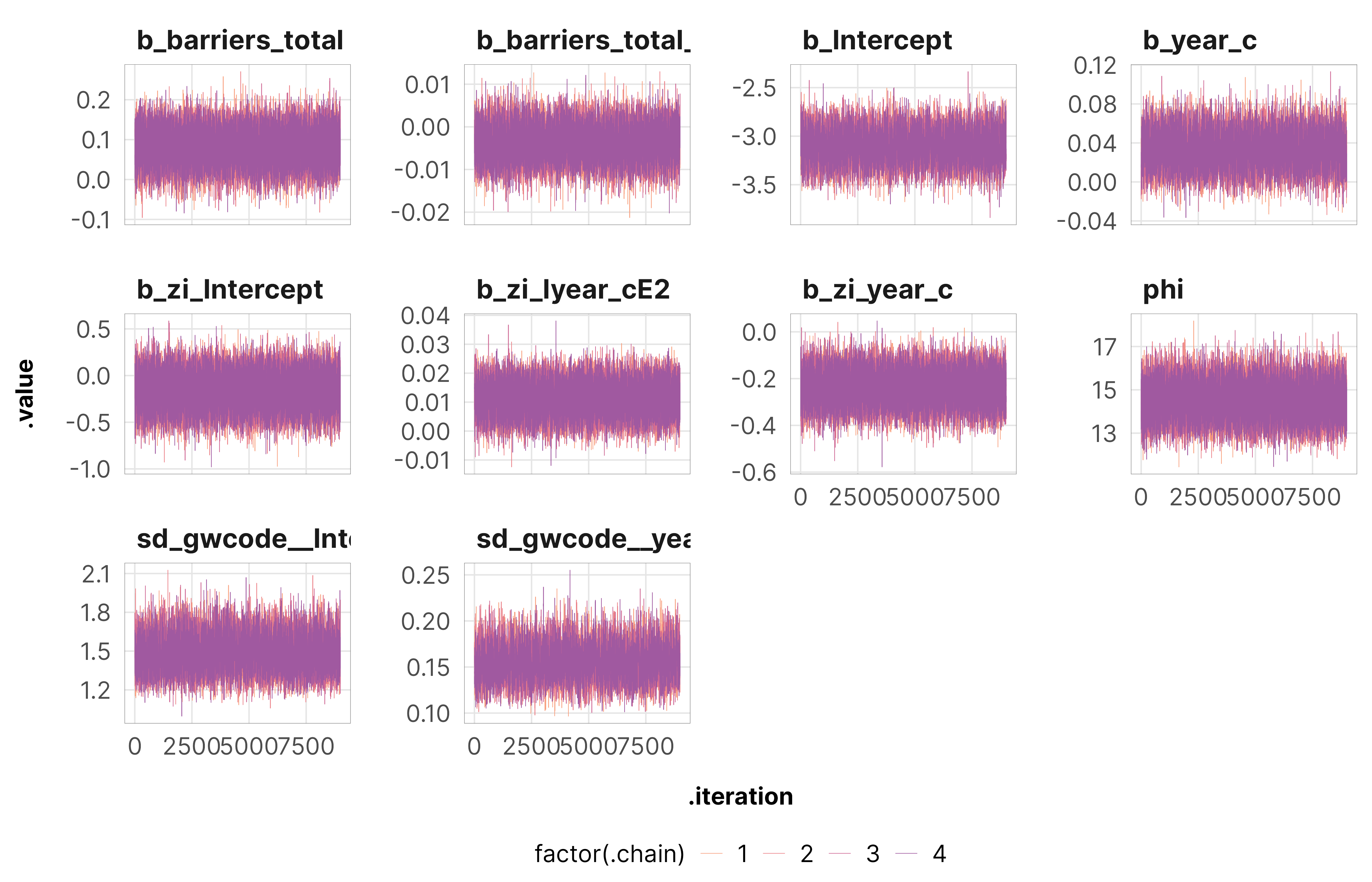
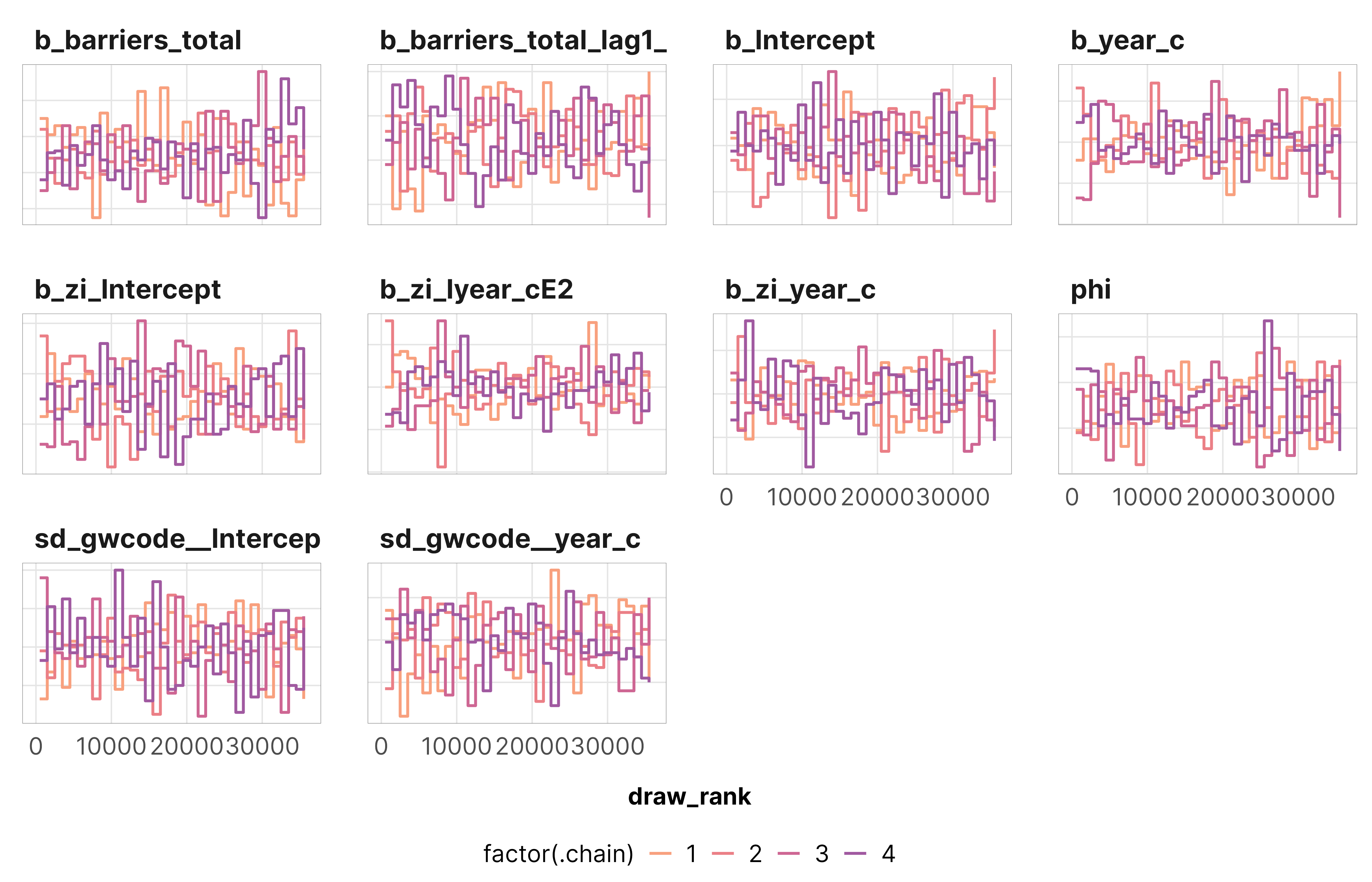
To check that everything converged nicely, we check some diagnostics for the outcome models for the total barriers treatment for domestic NGO recipients. All the other models look basically the same as this—everything’s fine.

Code

m_recip_outcome_total_dom$model %>% 
  gather_draws(`^b_.*|^sd_.*|^phi`, regex = TRUE) %>% 
  ggplot(aes(x = .iteration, y = .value, color = factor(.chain))) +
  geom_line(linewidth = 0.1) +
  scale_color_manual(values = clrs$Sunset[3:6]) +
  facet_wrap(vars(.variable), scales = "free_y") +
  theme_donors()

Code

m_recip_outcome_total_dom$model %>% 
  gather_draws(`^b_.*|^sd_.*|^phi`, regex = TRUE) %>% 
  group_by(.variable) %>% 
  mutate(draw_rank = rank(.value)) %>% 
  ggplot(aes(x = draw_rank, color = factor(.chain))) +
  stat_bin(geom = "step", binwidth = 1000, position = position_identity(), boundary = 0) +
  scale_color_manual(values = clrs$Sunset[3:6]) +
  facet_wrap(vars(.variable), scales = "free_y") +
  theme_donors() +
  theme(axis.text.y = element_blank(), axis.title.y = element_blank(), axis.ticks.y = element_blank())

Code

withr::with_seed(1234, {
  pp_check(m_recip_outcome_total_dom$model, ndraws = 20) +
    labs(x = "Proportion of aid to domestic NGOs",
         title = "Outcome model") +
    theme_donors() +
    coord_cartesian(xlim = c(0, 1))
})

Analyzing the posterior

Average treatment effects

Just like the other hypotheses, we look at conditional effects here, or the effect of these various kinds of civil society restrictions in a typical country (where the country-specific $b$ offsets are set to zero).

% of aid to domestic NGO recipients
% of aid to foreign NGO recipients

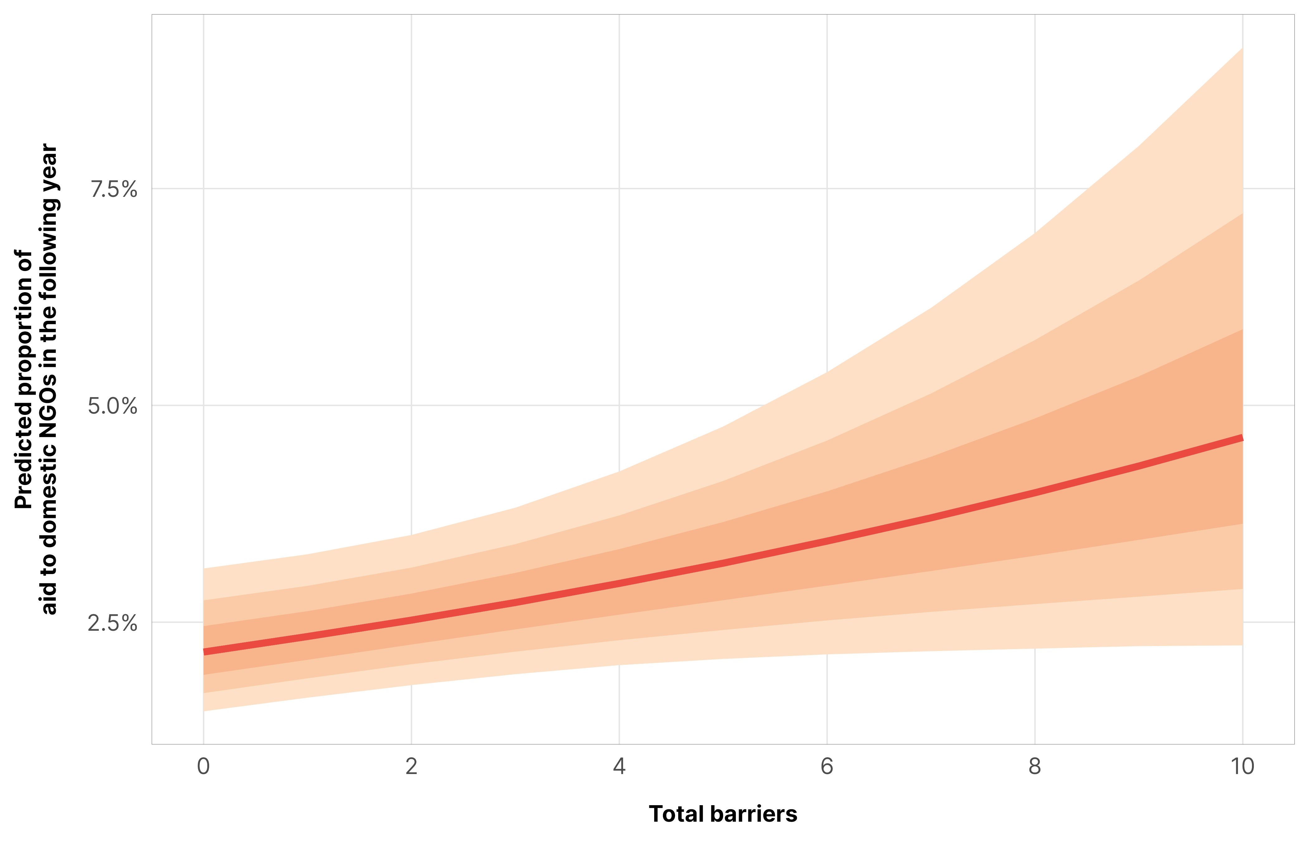
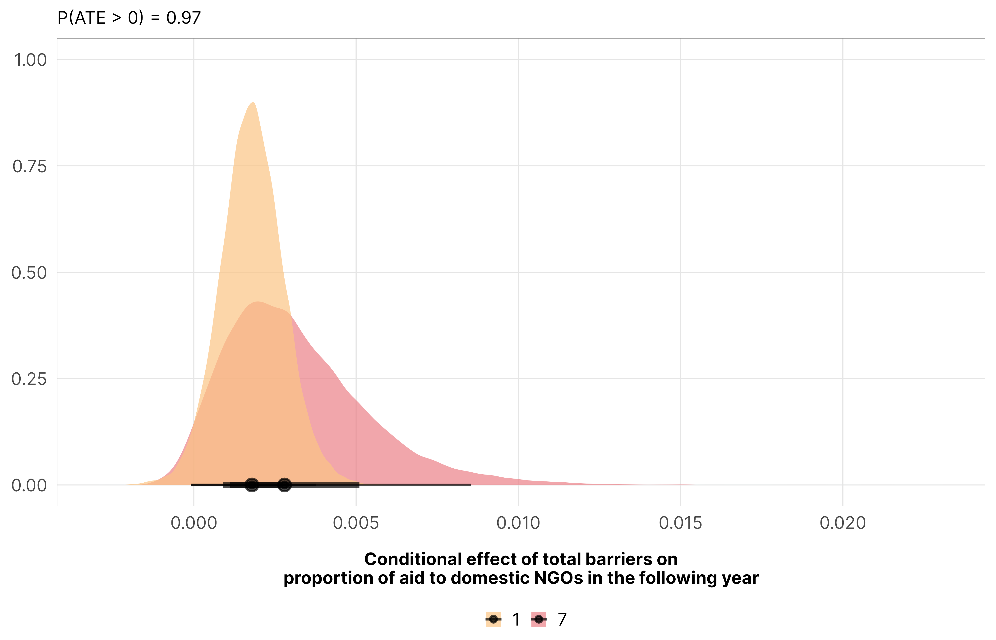
Additional barriers of any type lead to a tiny more aid to domestic NGOs, with an average increase of 0.18 percentage points (and the probability of being greater than zero is 0.97). This encompasses multiple countervailing trends though, since barriers to advocacy decrease the amount and other barriers increase it.

Code

m_recip_outcome_total_dom$model %>% 
  epred_draws(newdata = datagrid(model = m_recip_outcome_total_dom$model,
                                 year_c = 0,
                                 barriers_total = seq(0, 10, 1)),
              re_formula = NA) %>% 
  ggplot(aes(x = barriers_total, y = .epred)) +
  stat_lineribbon(color = clrs$Peach[7]) +
  scale_x_continuous(breaks = seq(0, 10, by = 2)) +
  scale_y_continuous(labels = label_percent()) +
  scale_fill_manual(values = clrs$Peach[1:3]) +
  guides(fill = "none") +
  labs(x = "Total barriers", y = "Predicted proportion of\naid to domestic NGOs in the following year") +
  theme_donors()

Code

mfx_recip_cfx_multiple_dom$total %>% 
  select(barriers_total, dydx, conf.low, conf.high)
##    barriers_total    dydx  conf.low conf.high
## 1               0 0.00166 -9.56e-05   0.00327
## 2               1 0.00179 -9.52e-05   0.00376
## 3               2 0.00193 -9.48e-05   0.00434
## 4               3 0.00208 -9.45e-05   0.00499
## 5               4 0.00225 -9.41e-05   0.00574
## 6               5 0.00242 -9.38e-05   0.00657
## 7               6 0.00260 -9.34e-05   0.00749
## 8               7 0.00279 -9.31e-05   0.00854
## 9               8 0.00300 -9.27e-05   0.00967
## 10              9 0.00321 -9.23e-05   0.01086
## 11             10 0.00344 -9.20e-05   0.01218

Code

mfx_total_p_direction_dom <- mfx_recip_cfx_multiple_dom$total %>% 
  posteriordraws() %>% 
  filter(barriers_total == 1) %>% 
  summarize(pd = sum(draw < 0) / n()) %>% 
  mutate(pd_short = round(pd, 2))

Code

mfx_recip_cfx_multiple_dom$total %>% 
  posteriordraws() %>% 
  filter(barriers_total %in% c(1, 7)) %>% 
  pivot_longer(draw) %>% 
  ggplot(aes(x = value, fill = factor(barriers_total))) +
  stat_halfeye(alpha = 0.7) +
  scale_x_continuous(labels = label_number(style_negative = "minus")) +
  scale_fill_manual(values = clrs$Sunset[c(2, 4, 6)]) +
  labs(x = "Conditional effect of total barriers on\nproportion of aid to domestic NGOs in the following year", y = NULL,
       subtitle = glue("P(ATE > 0) = {1 - pull(mfx_total_p_direction_dom, pd_short)}"), fill = NULL) +
  theme_donors()

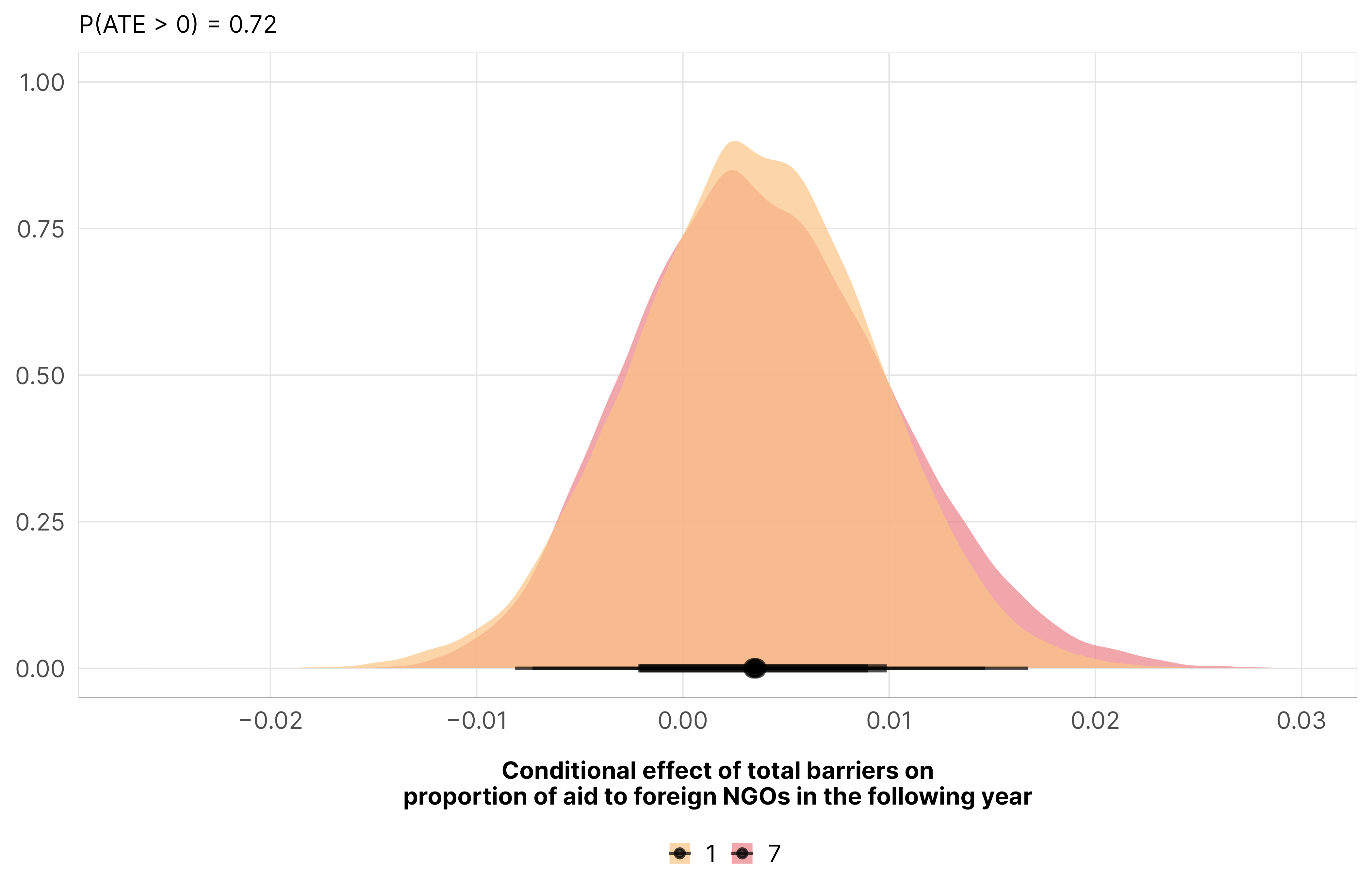
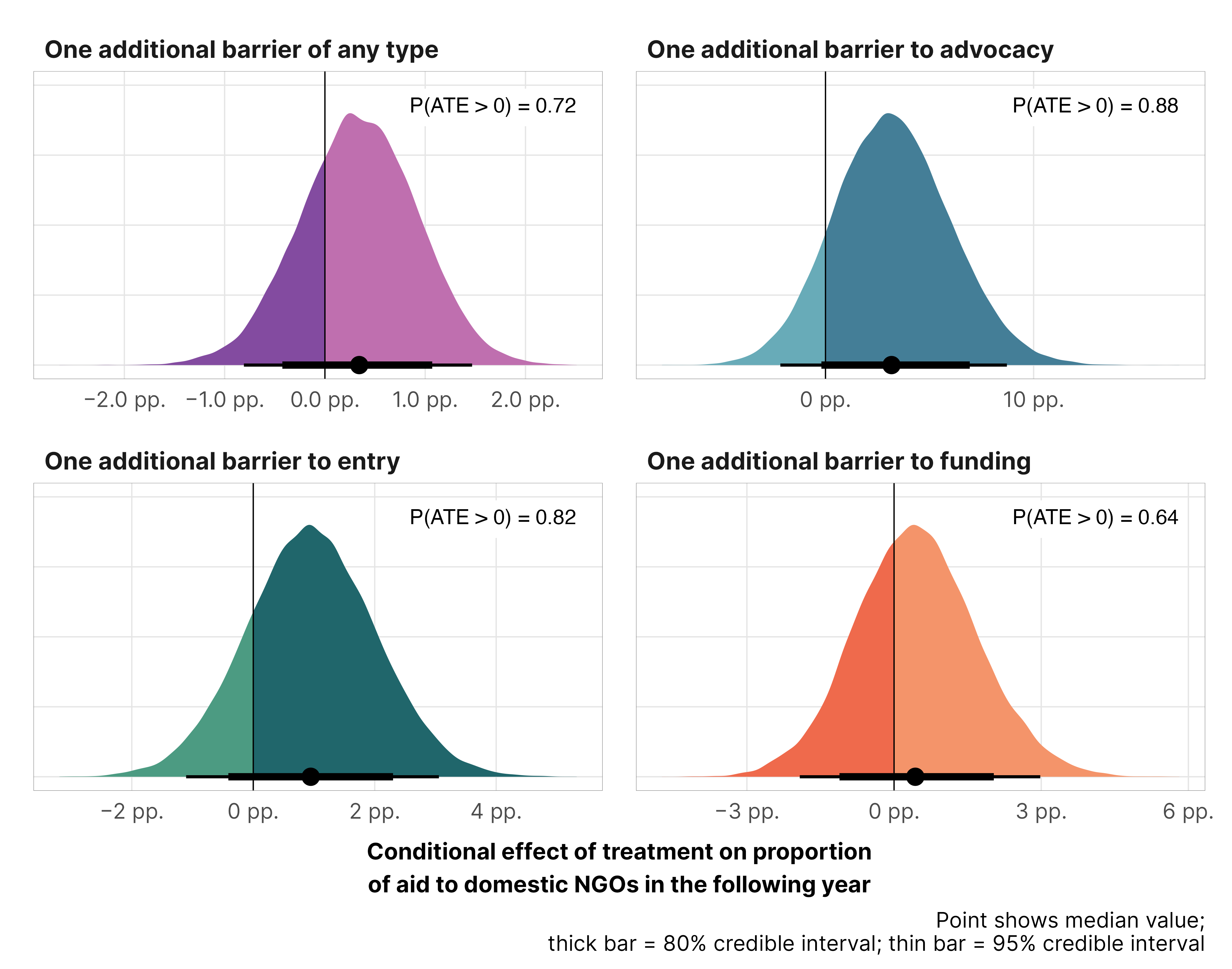
Additional legal barriers of any type slightly increase the proportion allocated to foreign NGOs by 0.34 percentage points, but the probability that that’s greater than zero is only 0.72.

Code

m_recip_outcome_total_foreign$model %>% 
  epred_draws(newdata = datagrid(model = m_recip_outcome_total_foreign$model,
                                 year_c = 0,
                                 barriers_total = seq(0, 10, 1)),
              re_formula = NA) %>% 
  ggplot(aes(x = barriers_total, y = .epred)) +
  stat_lineribbon(color = clrs$Peach[7]) +
  scale_x_continuous(breaks = seq(0, 10, by = 2)) +
  scale_y_continuous(labels = label_percent()) +
  scale_fill_manual(values = clrs$Peach[1:3]) +
  guides(fill = "none") +
  labs(x = "Total barriers", y = "Predicted proportion of\naid to foreign NGOs in the following year") +
  theme_donors()

Code

mfx_recip_cfx_multiple_foreign$total %>% 
  select(barriers_total, dydx, conf.low, conf.high)
##    barriers_total    dydx conf.low conf.high
## 1               0 0.00340 -0.00824    0.0142
## 2               1 0.00342 -0.00813    0.0146
## 3               2 0.00345 -0.00802    0.0151
## 4               3 0.00347 -0.00788    0.0155
## 5               4 0.00350 -0.00775    0.0159
## 6               5 0.00352 -0.00760    0.0162
## 7               6 0.00355 -0.00745    0.0165
## 8               7 0.00357 -0.00729    0.0167
## 9               8 0.00359 -0.00712    0.0169
## 10              9 0.00361 -0.00697    0.0170
## 11             10 0.00363 -0.00680    0.0170

Code

mfx_total_p_direction_foreign <- mfx_recip_cfx_multiple_foreign$total %>% 
  posteriordraws() %>% 
  filter(barriers_total == 1) %>% 
  summarize(pd = sum(draw < 0) / n()) %>% 
  mutate(pd_short = round(pd, 2))

Code

mfx_recip_cfx_multiple_foreign$total %>% 
  posteriordraws() %>% 
  filter(barriers_total %in% c(1, 7)) %>% 
  pivot_longer(draw) %>% 
  ggplot(aes(x = value, fill = factor(barriers_total))) +
  stat_halfeye(alpha = 0.7) +
  scale_x_continuous(labels = label_number(style_negative = "minus")) +
  scale_fill_manual(values = clrs$Sunset[c(2, 4, 6)]) +
  labs(x = "Conditional effect of total barriers on\nproportion of aid to foreign NGOs in the following year", y = NULL,
       subtitle = glue("P(ATE > 0) = {1 - pull(mfx_total_p_direction_foreign, pd_short)}"), fill = NULL) +
  theme_donors()

% of aid to domestic NGO recipients
% of aid to foreign NGO recipients

The story of advocacy laws is fascinating!. Additional barriers to advocacy decrease the amount of aid allocated to domestic NGOs, with a marginal effect of -0.6 percentage points (and a probability of being less than zero of 0.92).

Code

m_recip_outcome_advocacy_dom$model %>% 
  epred_draws(newdata = datagrid(model = m_recip_outcome_advocacy_dom$model,
                                 year_c = 0,
                                 advocacy = seq(0, 2, 1)),
              re_formula = NA) %>% 
  ggplot(aes(x = advocacy, y = .epred)) +
  stat_lineribbon(color = clrs$Peach[7]) +
  scale_x_continuous(breaks = 0:2) +
  scale_y_continuous(labels = label_percent()) +
  scale_fill_manual(values = clrs$Peach[1:3]) +
  guides(fill = "none") +
  labs(x = "Barriers to advocacy", y = "Predicted proportion of\naid to domestic NGOs in the following year") +
  theme_donors()

Code

mfx_recip_cfx_multiple_dom$advocacy %>% 
  select(advocacy, dydx, conf.low, conf.high)
##   advocacy     dydx conf.low conf.high
## 1        0 -0.00780 -0.02361   0.00269
## 2        1 -0.00612 -0.01430   0.00294
## 3        2 -0.00470 -0.00882   0.00322

Code

mfx_advocacy_p_direction_dom <- mfx_recip_cfx_multiple_dom$advocacy %>% 
  posteriordraws() %>% 
  filter(advocacy == 1) %>% 
  summarize(pd = sum(draw > 0) / n()) %>% 
  mutate(pd_short = round(pd, 2))

Code

mfx_recip_cfx_multiple_dom$advocacy %>% 
  posteriordraws() %>% 
  pivot_longer(draw) %>% 
  ggplot(aes(x = value, fill = factor(advocacy))) +
  stat_halfeye(alpha = 0.7) +
  scale_x_continuous(labels = label_number(style_negative = "minus")) +
  scale_fill_manual(values = clrs$Sunset[c(2, 4, 6)]) +
  labs(x = "Conditional effect of barriers to advocacy on\nproportion of aid to domestic NGOs in the following year", y = NULL,
       subtitle = glue("P(ATE < 0) = {1 - pull(mfx_advocacy_p_direction_dom, pd_short)}"), fill = NULL) +
  theme_donors()

In contrast, however, additional barriers to advocacy increase the amount of aid allocated to foreign NGOs, with a marginal effect of 3 percentage points (and a probability of being greater than zero of 0.88)

Code

m_recip_outcome_advocacy_foreign$model %>% 
  epred_draws(newdata = datagrid(model = m_recip_outcome_advocacy_foreign$model,
                                 year_c = 0,
                                 advocacy = seq(0, 2, 1)),
              re_formula = NA) %>% 
  ggplot(aes(x = advocacy, y = .epred)) +
  stat_lineribbon(color = clrs$Peach[7]) +
  scale_x_continuous(breaks = 0:2) +
  scale_y_continuous(labels = label_percent()) +
  scale_fill_manual(values = clrs$Peach[1:3]) +
  guides(fill = "none") +
  labs(x = "Barriers to advocacy", y = "Predicted proportion of\naid to foreign NGOs in the following year") +
  theme_donors()

Code

mfx_recip_cfx_multiple_foreign$advocacy %>% 
  select(advocacy, dydx, conf.low, conf.high)
##   advocacy   dydx conf.low conf.high
## 1        0 0.0299  -0.0217    0.0765
## 2        1 0.0317  -0.0208    0.0884
## 3        2 0.0332  -0.0197    0.0923

Code

mfx_advocacy_p_direction_foreign <- mfx_recip_cfx_multiple_foreign$advocacy %>% 
  posteriordraws() %>% 
  filter(advocacy == 1) %>% 
  summarize(pd = sum(draw > 0) / n()) %>% 
  mutate(pd_short = round(pd, 2))

Code

mfx_recip_cfx_multiple_foreign$advocacy %>% 
  posteriordraws() %>% 
  pivot_longer(draw) %>% 
  ggplot(aes(x = value, fill = factor(advocacy))) +
  stat_halfeye(alpha = 0.7) +
  scale_x_continuous(labels = label_number(style_negative = "minus")) +
  scale_fill_manual(values = clrs$Sunset[c(2, 4, 6)]) +
  labs(x = "Conditional effect of barriers to advocacy on\nproportion of aid to foreign NGOs in the following year", y = NULL,
       subtitle = glue("P(ATE > 0) = {pull(mfx_advocacy_p_direction_foreign, pd_short)}"), fill = NULL) +
  theme_donors()

% of aid to domestic NGO recipients
% of aid to foreign NGO recipients

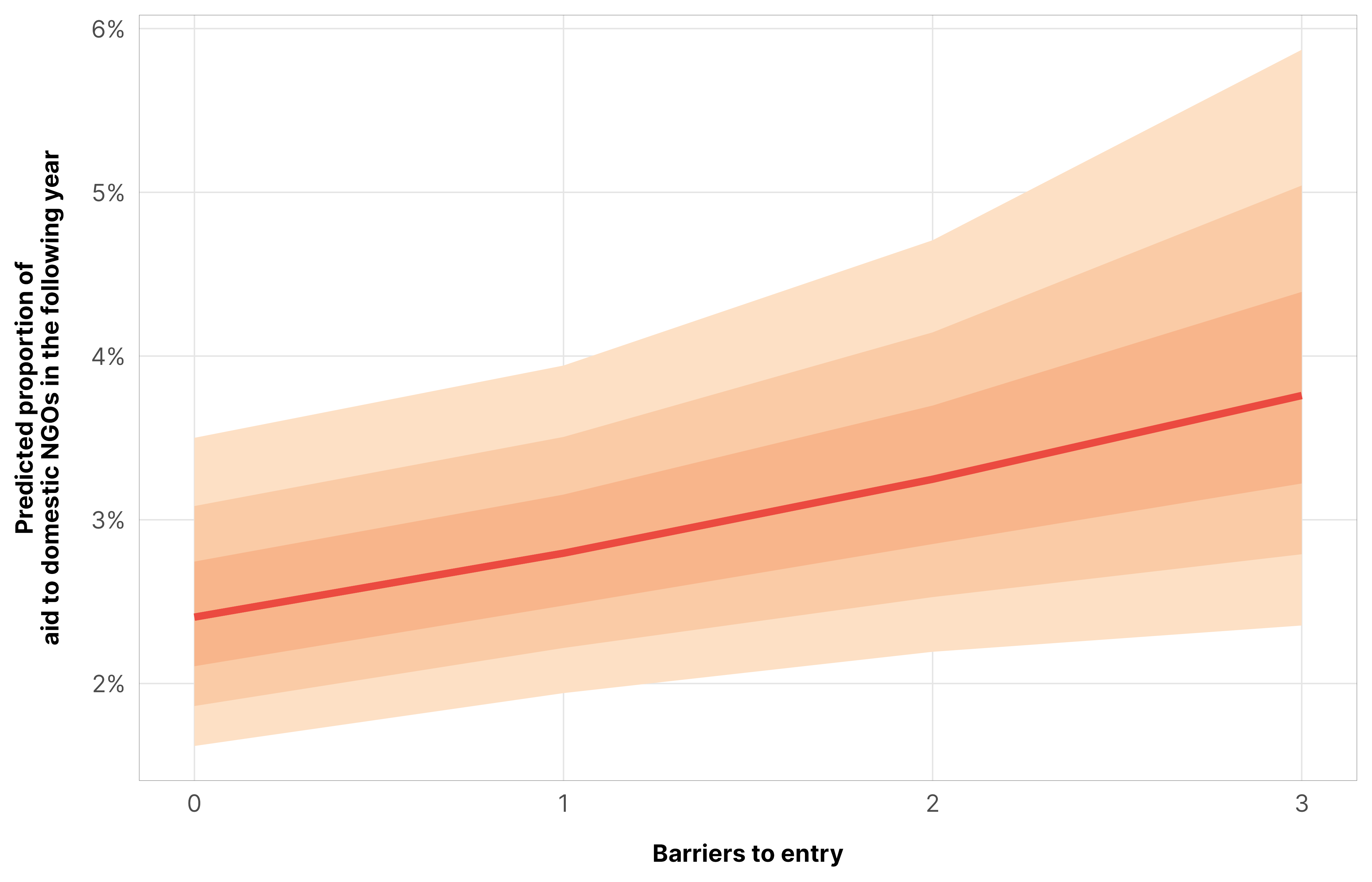
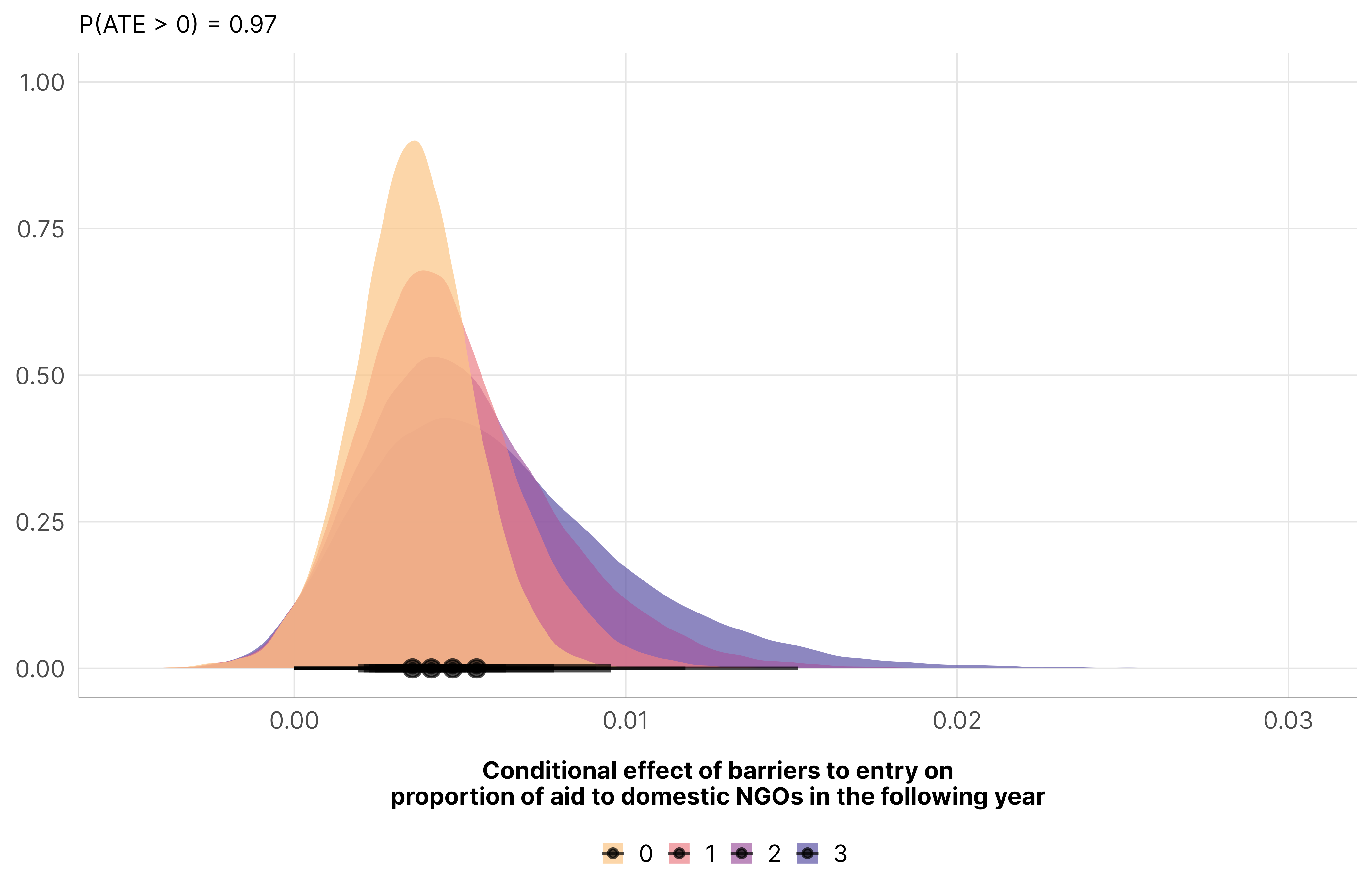
Additional barriers to entry increase the proportion of aid allocated to domestic NGOs, with a marginal effect of 0.4 percentage points (and a probability of being greater than zero of 0.97).

Code

m_recip_outcome_entry_dom$model %>% 
  epred_draws(newdata = datagrid(model = m_recip_outcome_entry_dom$model,
                                 year_c = 0,
                                 entry = seq(0, 3, 1)),
              re_formula = NA) %>% 
  ggplot(aes(x = entry, y = .epred)) +
  stat_lineribbon(color = clrs$Peach[7]) +
  scale_x_continuous(breaks = 0:3) +
  scale_y_continuous(labels = label_percent()) +
  scale_fill_manual(values = clrs$Peach[1:3]) +
  guides(fill = "none") +
  labs(x = "Barriers to entry", y = "Predicted proportion of\naid to domestic NGOs in the following year") +
  theme_donors()

Code

mfx_recip_cfx_multiple_dom$entry %>% 
  select(entry, dydx, conf.low, conf.high)
##   entry    dydx  conf.low conf.high
## 1     0 0.00357 -1.43e-05   0.00703
## 2     1 0.00414 -1.43e-05   0.00911
## 3     2 0.00478 -1.43e-05   0.01180
## 4     3 0.00550 -1.43e-05   0.01519

Code

mfx_entry_p_direction_dom <- mfx_recip_cfx_multiple_dom$entry %>% 
  posteriordraws() %>% 
  filter(entry == 1) %>% 
  summarize(pd = sum(draw > 0) / n()) %>% 
  mutate(pd_short = round(pd, 2))

Code

mfx_recip_cfx_multiple_dom$entry %>% 
  posteriordraws() %>% 
  pivot_longer(draw) %>% 
  ggplot(aes(x = value, fill = factor(entry))) +
  stat_halfeye(alpha = 0.7) +
  scale_x_continuous(labels = label_number(style_negative = "minus")) +
  scale_fill_manual(values = clrs$Sunset[c(2, 4, 6, 7)]) +
  labs(x = "Conditional effect of barriers to entry on\nproportion of aid to domestic NGOs in the following year", y = NULL,
       subtitle = glue("P(ATE > 0) = {pull(mfx_entry_p_direction_dom, pd_short)}"), fill = NULL) +
  theme_donors()

Barriers to entry kind of increase the amount of aid given to foreign NGOs too, but the signal is a little weaker and uncertain. The marginal effect is almost 1 percentage point (0.95), but the probability that that’s greater than zero is 0.82.

Code

m_recip_outcome_entry_foreign$model %>% 
  epred_draws(newdata = datagrid(model = m_recip_outcome_entry_foreign$model,
                                 year_c = 0,
                                 entry = seq(0, 3, 1)),
              re_formula = NA) %>% 
  ggplot(aes(x = entry, y = .epred)) +
  stat_lineribbon(color = clrs$Peach[7]) +
  scale_x_continuous(breaks = 0:3) +
  scale_y_continuous(labels = label_percent()) +
  scale_fill_manual(values = clrs$Peach[1:3]) +
  guides(fill = "none") +
  labs(x = "Barriers to entry", y = "Predicted proportion of\naid to foreign NGOs in the following year") +
  theme_donors()

Code

mfx_recip_cfx_multiple_foreign$entry %>% 
  select(entry, dydx, conf.low, conf.high)
##   entry    dydx conf.low conf.high
## 1     0 0.00927  -0.0114    0.0285
## 2     1 0.00947  -0.0112    0.0305
## 3     2 0.00965  -0.0109    0.0322
## 4     3 0.00982  -0.0106    0.0334

Code

mfx_entry_p_direction_foreign <- mfx_recip_cfx_multiple_foreign$entry %>% 
  posteriordraws() %>% 
  filter(entry == 1) %>% 
  summarize(pd = sum(draw > 0) / n()) %>% 
  mutate(pd_short = round(pd, 2))

Code

mfx_recip_cfx_multiple_foreign$entry %>% 
  posteriordraws() %>% 
  pivot_longer(draw) %>% 
  ggplot(aes(x = value, fill = factor(entry))) +
  stat_halfeye(alpha = 0.7) +
  scale_x_continuous(labels = label_number(style_negative = "minus")) +
  scale_fill_manual(values = clrs$Sunset[c(2, 4, 6, 7)]) +
  labs(x = "Conditional effect of barriers to entry on\nproportion of aid to foreign NGOs in the following year", y = NULL,
       subtitle = glue("P(ATE > 0) = {pull(mfx_entry_p_direction_foreign, pd_short)}"), fill = NULL) +
  theme_donors()

% of aid to domestic NGO recipients
% of aid to foreign NGO recipients

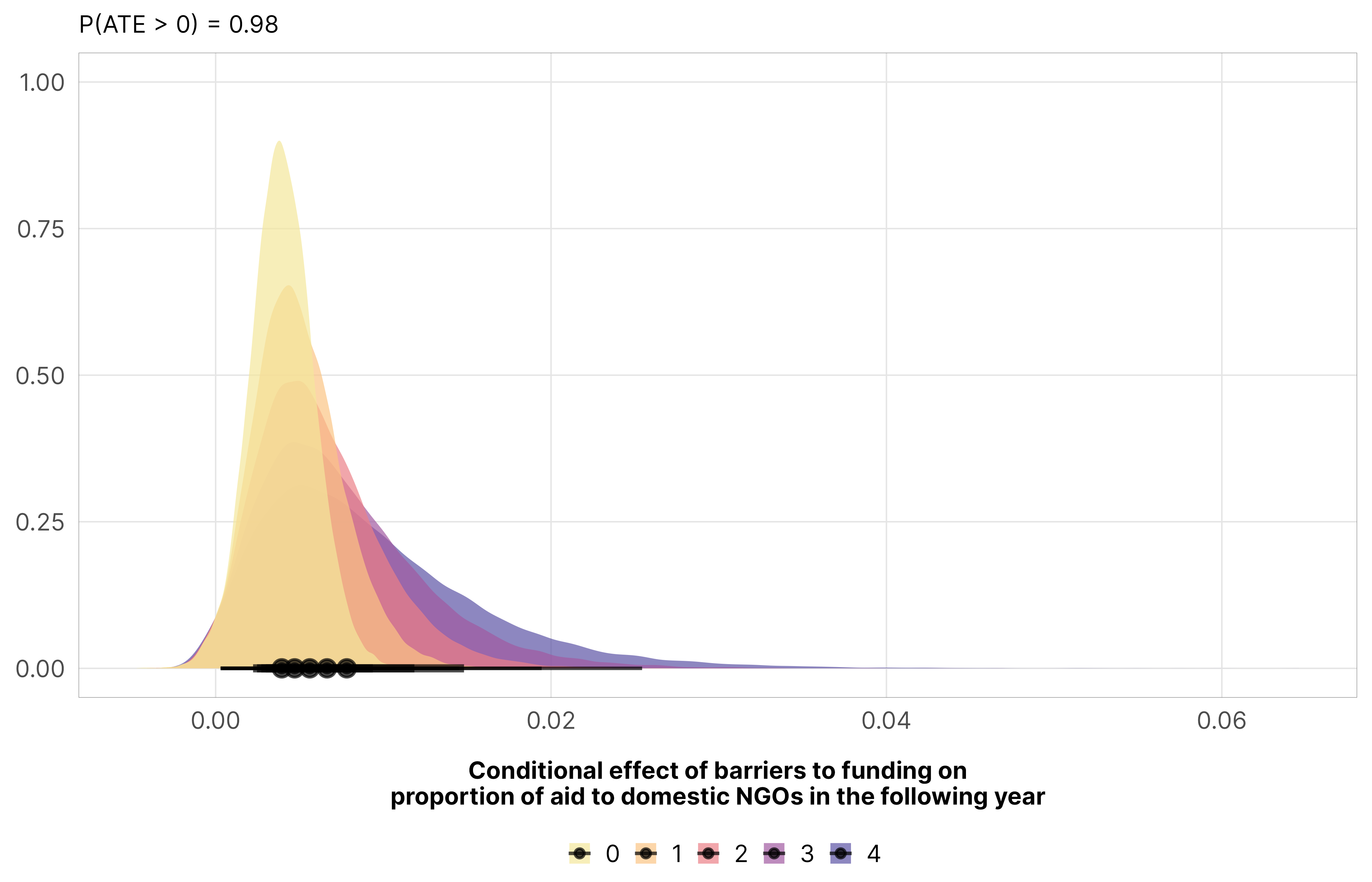
Additional barriers to funding increase the proportion of aid given to domestic NGOs, with a marginal effect of half a percentage point (0.47), which is definitely greater than zero (0.98).

Code

m_recip_outcome_funding_dom$model %>% 
  epred_draws(newdata = datagrid(model = m_recip_outcome_funding_dom$model,
                                 year_c = 0,
                                 funding = seq(0, 4, 1)),
              re_formula = NA) %>% 
  ggplot(aes(x = funding, y = .epred)) +
  stat_lineribbon(color = clrs$Peach[7]) +
  scale_x_continuous(breaks = 0:4) +
  scale_y_continuous(labels = label_percent()) +
  scale_fill_manual(values = clrs$Peach[1:3]) +
  guides(fill = "none") +
  labs(x = "Barriers to funding", y = "Predicted proportion of\naid to domestic NGOs in the following year") +
  theme_donors()

Code

mfx_recip_cfx_multiple_dom$funding %>% 
  select(funding, dydx, conf.low, conf.high)
##   funding    dydx conf.low conf.high
## 1       0 0.00394 0.000294    0.0078
## 2       1 0.00471 0.000297    0.0107
## 3       2 0.00561 0.000301    0.0145
## 4       3 0.00664 0.000304    0.0194
## 5       4 0.00782 0.000308    0.0254

Code

mfx_funding_p_direction_dom <- mfx_recip_cfx_multiple_dom$funding %>% 
  posteriordraws() %>% 
  filter(funding == 1) %>% 
  summarize(pd = sum(draw < 0) / n()) %>% 
  mutate(pd_short = round(pd, 2))

Code

mfx_recip_cfx_multiple_dom$funding %>% 
  posteriordraws() %>% 
  pivot_longer(draw) %>% 
  ggplot(aes(x = value, fill = factor(funding))) +
  stat_halfeye(alpha = 0.7) +
  scale_x_continuous(labels = label_number(style_negative = "minus")) +
  scale_fill_manual(values = clrs$Sunset[c(1, 2, 4, 6, 7)]) +
  labs(x = "Conditional effect of barriers to funding on\nproportion of aid to domestic NGOs in the following year", y = NULL,
       subtitle = glue("P(ATE > 0) = {1 - pull(mfx_funding_p_direction_dom, pd_short)}"), fill = NULL) +
  theme_donors()

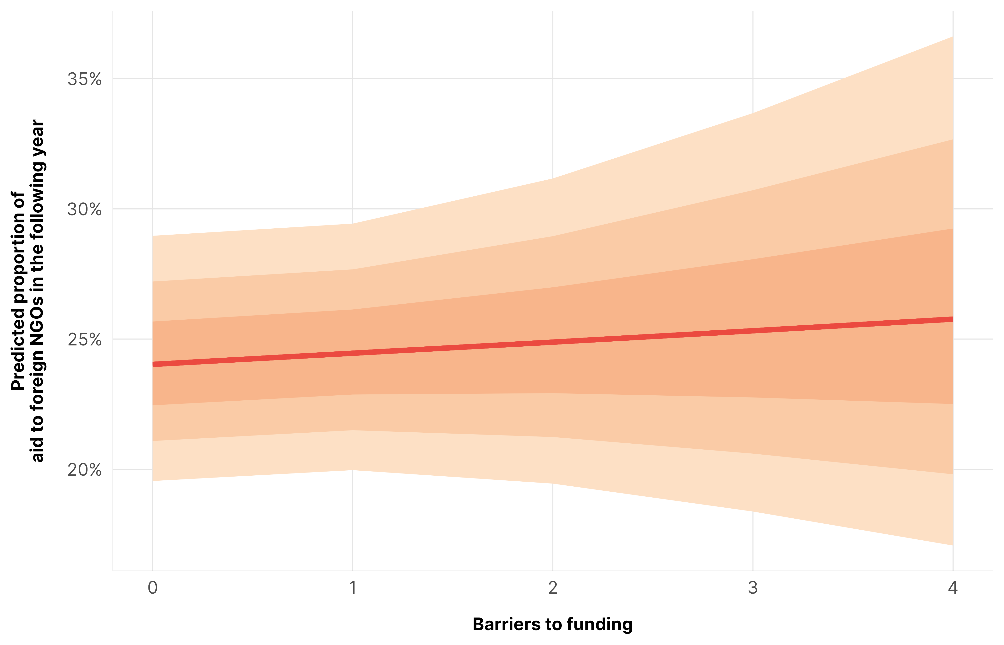
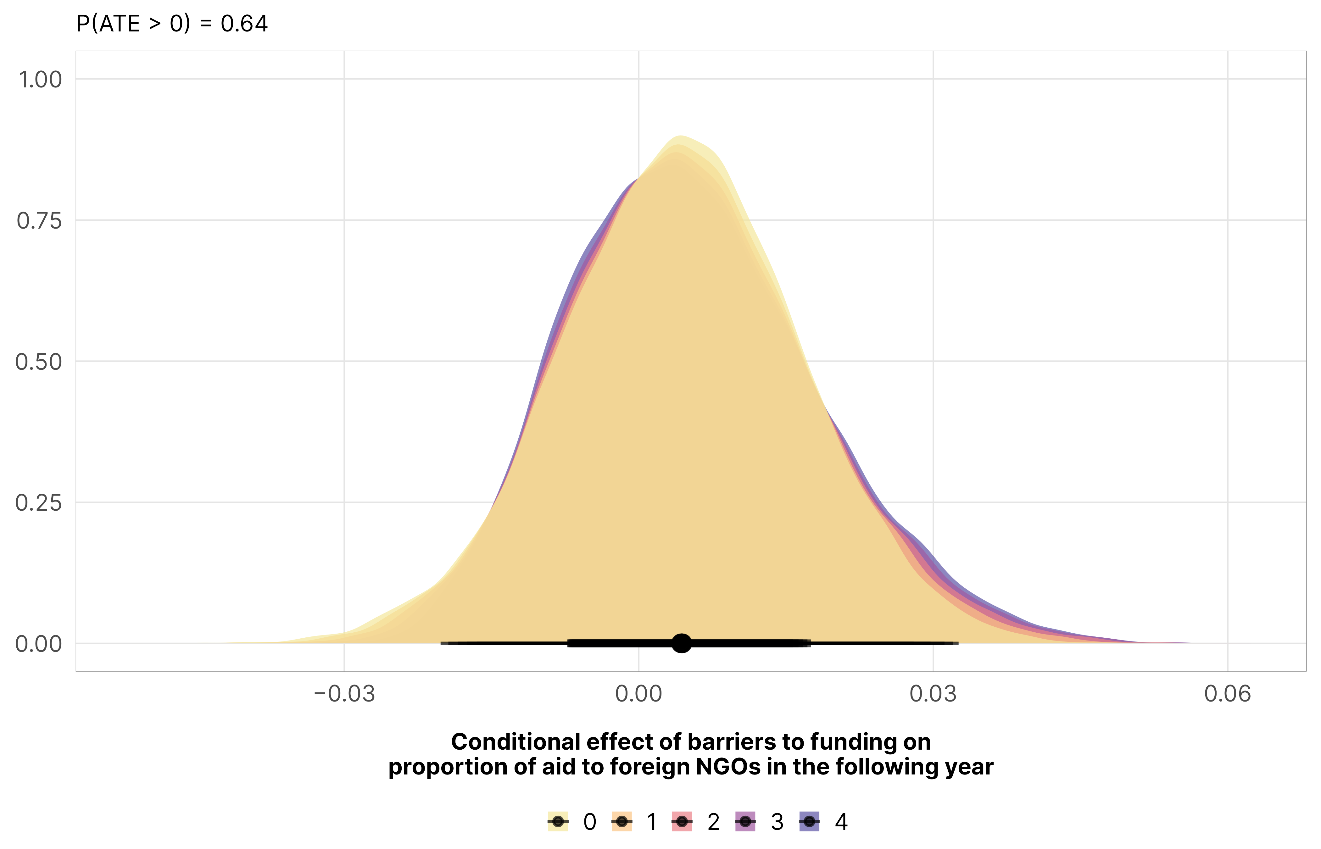
Additional barriers to funding also increase the amount of aid allocated to foreign NGOs, but the effect is far more uncertain here. The median is 0.43 percentage points, but the probability of being greater than zero is only 0.64—there’s a good chance it could be negative or nothing at all.

Code

m_recip_outcome_funding_foreign$model %>% 
  epred_draws(newdata = datagrid(model = m_recip_outcome_funding_foreign$model,
                                 year_c = 0,
                                 funding = seq(0, 4, 1)),
              re_formula = NA) %>% 
  ggplot(aes(x = funding, y = .epred)) +
  stat_lineribbon(color = clrs$Peach[7]) +
  scale_x_continuous(breaks = 0:4) +
  scale_y_continuous(labels = label_percent()) +
  scale_fill_manual(values = clrs$Peach[1:3]) +
  guides(fill = "none") +
  labs(x = "Barriers to funding", y = "Predicted proportion of\naid to foreign NGOs in the following year") +
  theme_donors()

Code

mfx_recip_cfx_multiple_foreign$funding %>% 
  select(funding, dydx, conf.low, conf.high)
##   funding    dydx conf.low conf.high
## 1       0 0.00429  -0.0202    0.0280
## 2       1 0.00433  -0.0194    0.0297
## 3       2 0.00437  -0.0184    0.0311
## 4       3 0.00442  -0.0175    0.0320
## 5       4 0.00445  -0.0165    0.0326

Code

mfx_funding_p_direction_foreign <- mfx_recip_cfx_multiple_foreign$funding %>% 
  posteriordraws() %>% 
  filter(funding == 1) %>% 
  summarize(pd = sum(draw < 0) / n()) %>% 
  mutate(pd_short = round(pd, 2))

Code

mfx_recip_cfx_multiple_foreign$funding %>% 
  posteriordraws() %>% 
  pivot_longer(draw) %>% 
  ggplot(aes(x = value, fill = factor(funding))) +
  stat_halfeye(alpha = 0.7) +
  scale_x_continuous(labels = label_number(style_negative = "minus")) +
  scale_fill_manual(values = clrs$Sunset[c(1, 2, 4, 6, 7)]) +
  labs(x = "Conditional effect of barriers to funding on\nproportion of aid to foreign NGOs in the following year", y = NULL,
       subtitle = glue("P(ATE > 0) = {1 - pull(mfx_funding_p_direction_foreign, pd_short)}"), fill = NULL) +
  theme_donors()

% of aid to domestic NGO recipients
% of aid to foreign NGO recipients

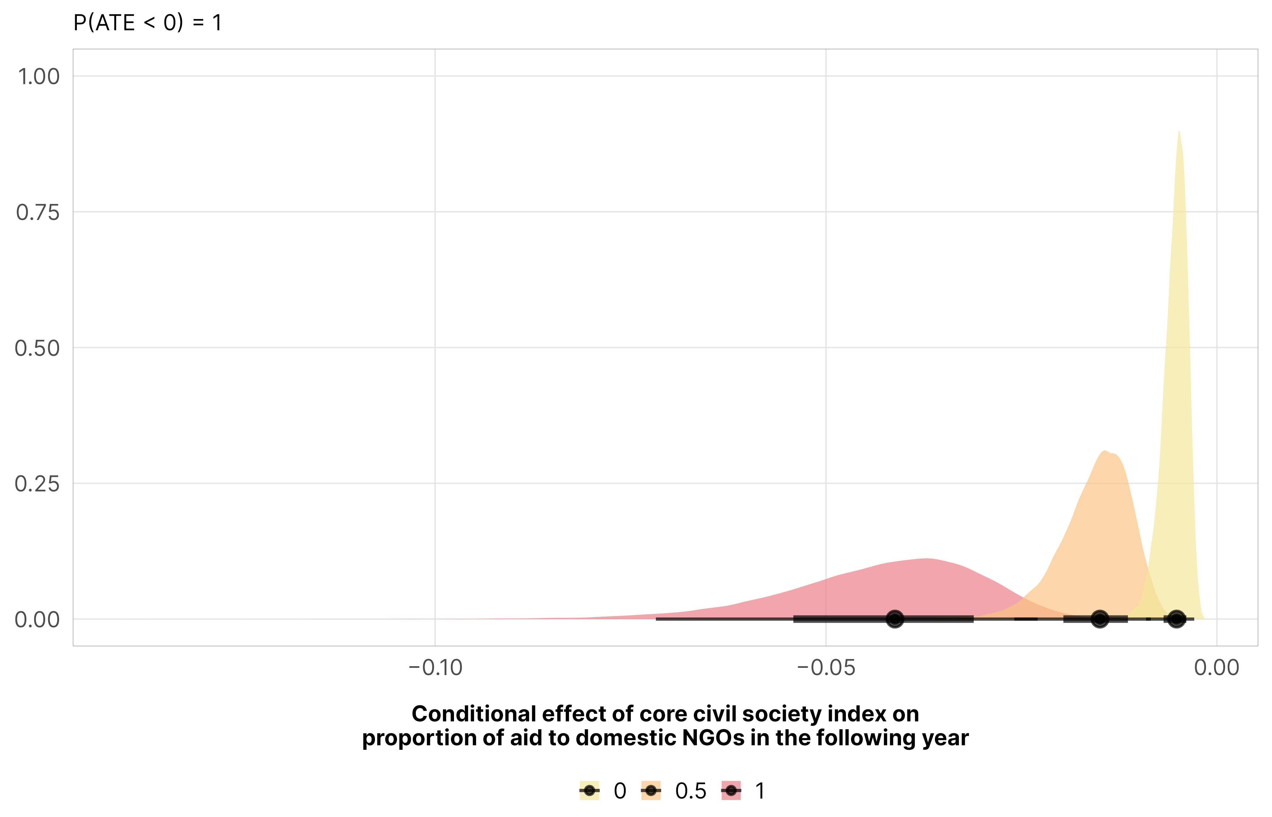
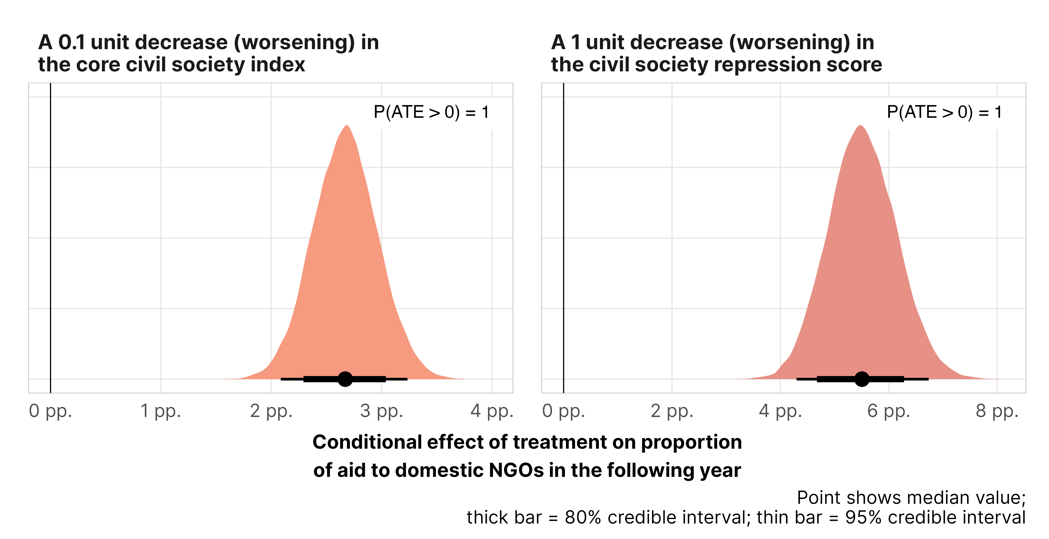
De facto civil society regulations tell a slightly different story. As the general legal environment gets worse, the proportion of aid allocated to dometic NGOs decreases, with a marginal effect of 0.15 percentage points (and a 100% probability of being positive).

Code

m_recip_outcome_ccsi_dom$model_50 %>% 
  epred_draws(newdata = datagrid(model = m_recip_outcome_ccsi_dom$model_50,
                                 year_c = 0,
                                 v2xcs_ccsi = seq(1, 0, -0.1)),
              re_formula = NA) %>% 
  ggplot(aes(x = v2xcs_ccsi, y = .epred)) +
  stat_lineribbon(color = clrs$Peach[7]) +
  scale_x_reverse() +
  scale_y_continuous(labels = label_percent()) +
  scale_fill_manual(values = clrs$Peach[1:3]) +
  guides(fill = "none") +
  labs(x = "Core civil society index", y = "Predicted proportion of\naid to domestic NGOs in the following year",
       caption = "**x-axis reversed**; lower values represent worse respect for civil society") +
  theme_donors() +
  theme(plot.caption = element_markdown())

Code

mfx_recip_cfx_multiple_dom$ccsi %>% 
  select(v2xcs_ccsi, dydx, conf.low, conf.high)
##   v2xcs_ccsi    dydx conf.low conf.high
## 1        0.0 0.00516  0.00291   0.00906
## 2        0.5 0.01496  0.00846   0.02591
## 3        1.0 0.04118  0.02294   0.07176

Code

mfx_ccsi_p_direction_dom <- mfx_recip_cfx_multiple_dom$ccsi %>% 
  posteriordraws() %>% 
  filter(v2xcs_ccsi == 0.5) %>% 
  summarize(pd = sum(draw < 0) / n()) %>% 
  mutate(pd_short = round(pd, 2))

Code

mfx_recip_cfx_multiple_dom$ccsi %>% 
  posteriordraws() %>% 
  mutate(draw = -draw) %>% 
  pivot_longer(draw) %>% 
  ggplot(aes(x = value, fill = factor(v2xcs_ccsi))) +
  stat_halfeye(alpha = 0.7) +
  scale_x_continuous(labels = label_number(style_negative = "minus")) +
  scale_fill_manual(values = clrs$Sunset[c(1, 2, 4, 6, 7)]) +
  labs(x = "Conditional effect of core civil society index on\nproportion of aid to domestic NGOs in the following year", y = NULL,
       subtitle = glue("P(ATE < 0) = {1 - pull(mfx_ccsi_p_direction_dom, pd_short)}"), fill = NULL) +
  theme_donors()

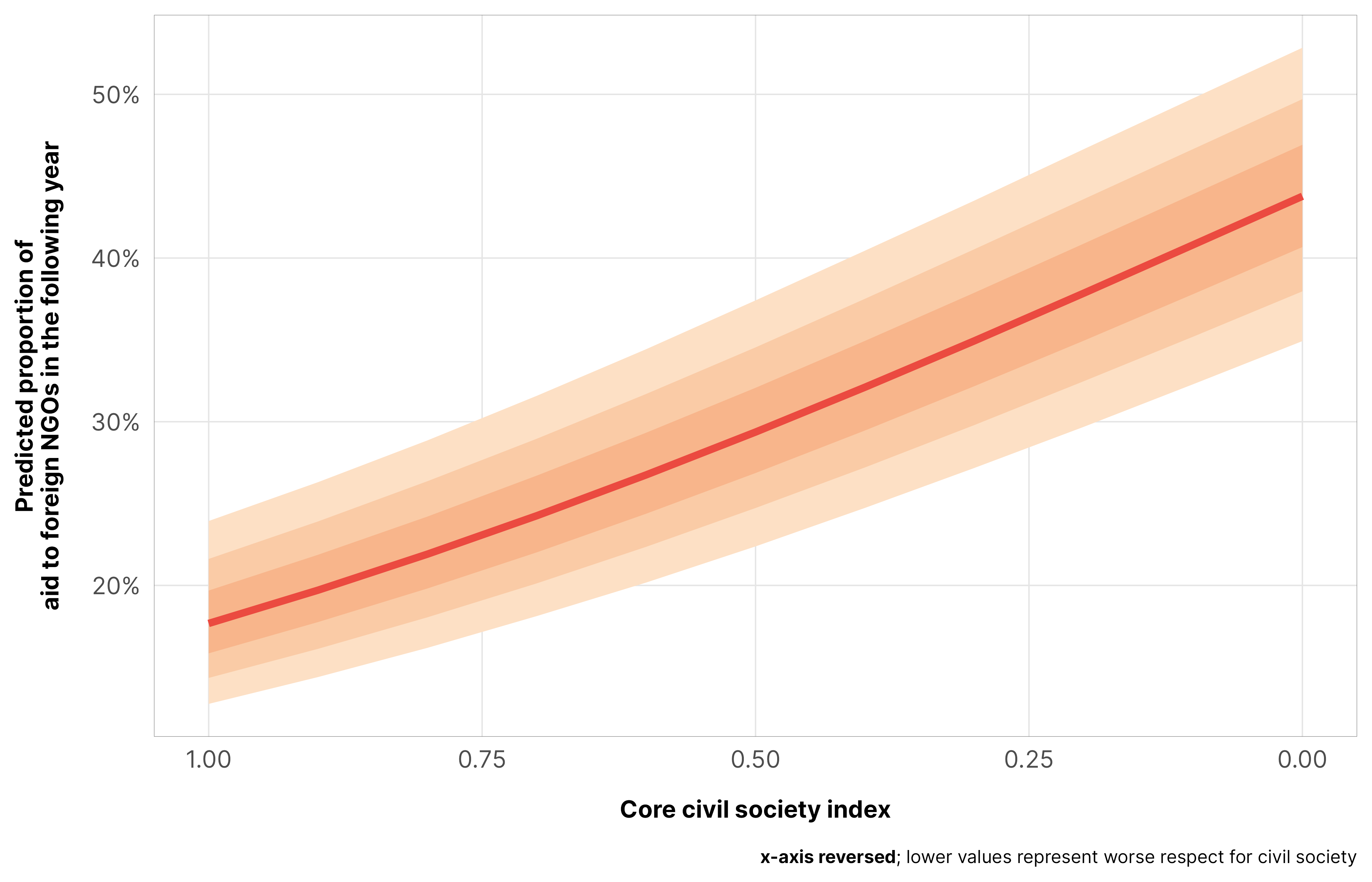
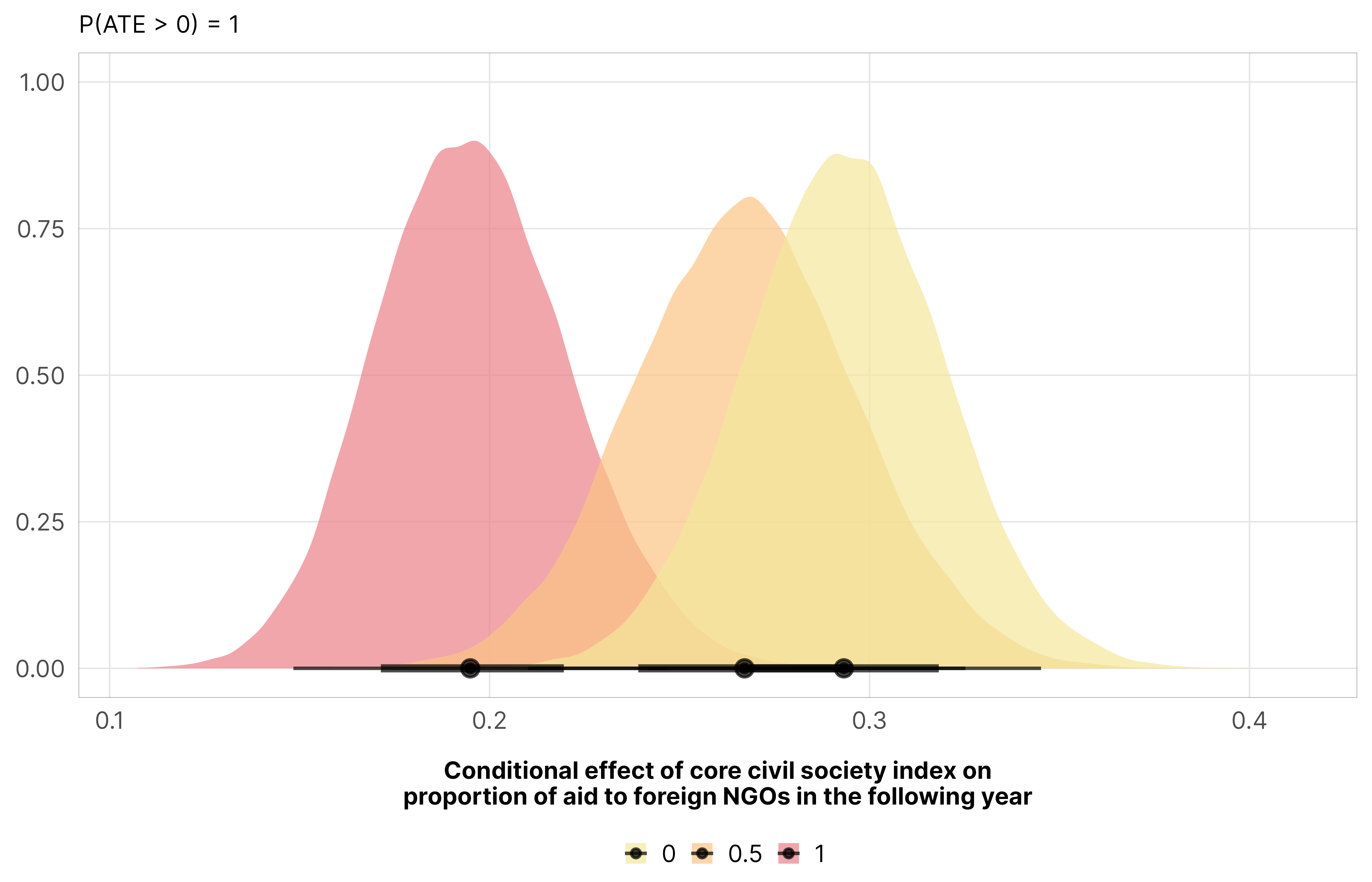
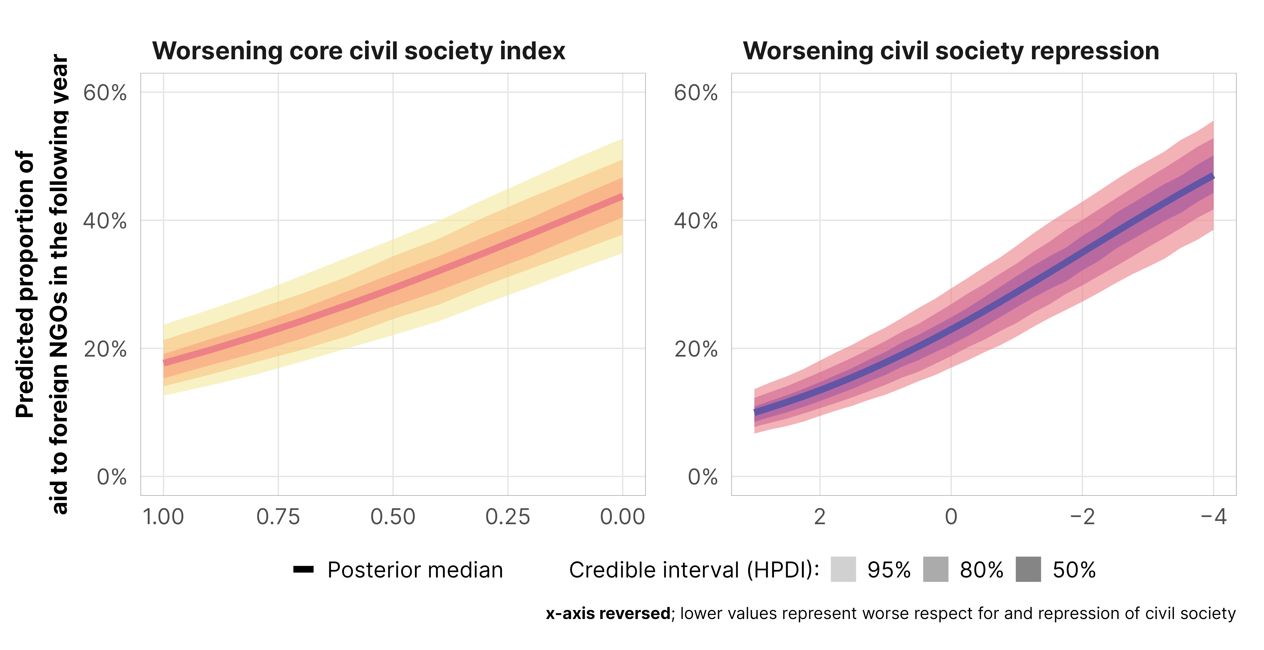
In contrast, a worsening environment for civil society causes a substantial increase in the proportion of aid allocated to foreign NGOs, with a huge marginal effect of 2.7 percentage points (and 100% chance of being positive). USAID seems to rely heavily on foreign NGOs in countries with restrictive civil society.

Code

m_recip_outcome_ccsi_foreign$model_50 %>% 
  epred_draws(newdata = datagrid(model = m_recip_outcome_ccsi_foreign$model_50,
                                 year_c = 0,
                                 v2xcs_ccsi = seq(0, 1, 0.1)),
              re_formula = NA) %>% 
  ggplot(aes(x = v2xcs_ccsi, y = .epred)) +
  stat_lineribbon(color = clrs$Peach[7]) +
  scale_x_reverse() +
  scale_y_continuous(labels = label_percent()) +
  scale_fill_manual(values = clrs$Peach[1:3]) +
  guides(fill = "none") +
  labs(x = "Core civil society index", y = "Predicted proportion of\naid to foreign NGOs in the following year",
       caption = "**x-axis reversed**; lower values represent worse respect for civil society") +
  theme_donors() +
  theme(plot.caption = element_markdown())

Code

mfx_recip_cfx_multiple_foreign$ccsi %>% 
  select(v2xcs_ccsi, dydx, conf.low, conf.high)
##   v2xcs_ccsi   dydx conf.low conf.high
## 1        0.0 -0.293   -0.345    -0.242
## 2        0.5 -0.267   -0.325    -0.210
## 3        1.0 -0.195   -0.247    -0.148

Code

mfx_ccsi_p_direction_foreign <- mfx_recip_cfx_multiple_foreign$ccsi %>% 
  posteriordraws() %>% 
  filter(v2xcs_ccsi == 0.5) %>% 
  summarize(pd = sum(draw < 0) / n()) %>% 
  mutate(pd_short = round(pd, 2))

Code

mfx_recip_cfx_multiple_foreign$ccsi %>% 
  posteriordraws() %>% 
  mutate(draw = -draw) %>% 
  pivot_longer(draw) %>% 
  ggplot(aes(x = value, fill = factor(v2xcs_ccsi))) +
  stat_halfeye(alpha = 0.7) +
  scale_fill_manual(values = clrs$Sunset[c(1, 2, 4, 6, 7)]) +
  labs(x = "Conditional effect of core civil society index on\nproportion of aid to foreign NGOs in the following year", y = NULL,
       subtitle = glue("P(ATE > 0) = {pull(mfx_ccsi_p_direction_foreign, pd_short)}"), fill = NULL) +
  theme_donors()

% of aid to domestic NGO recipients
% of aid to foreign NGO recipients

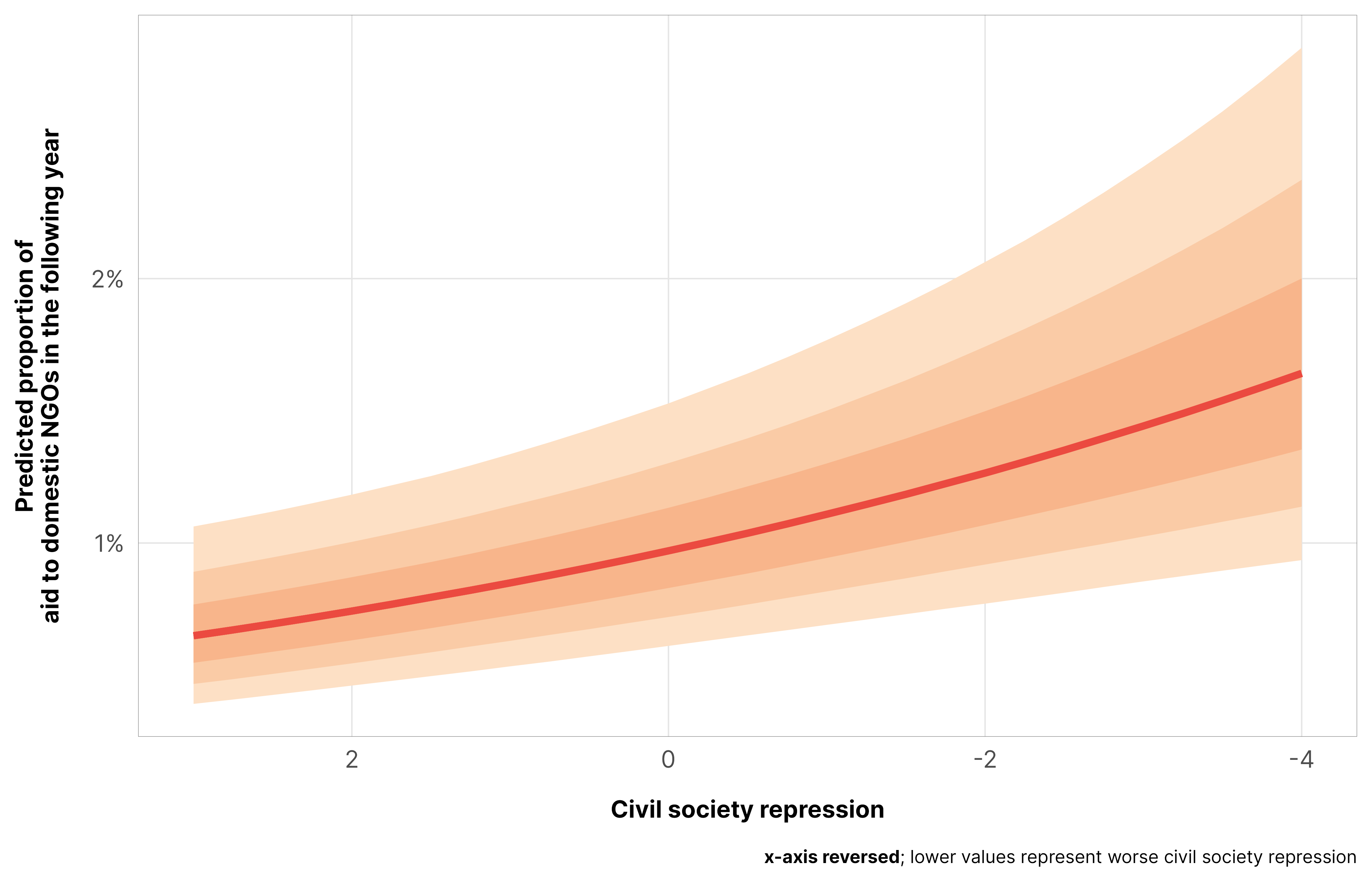
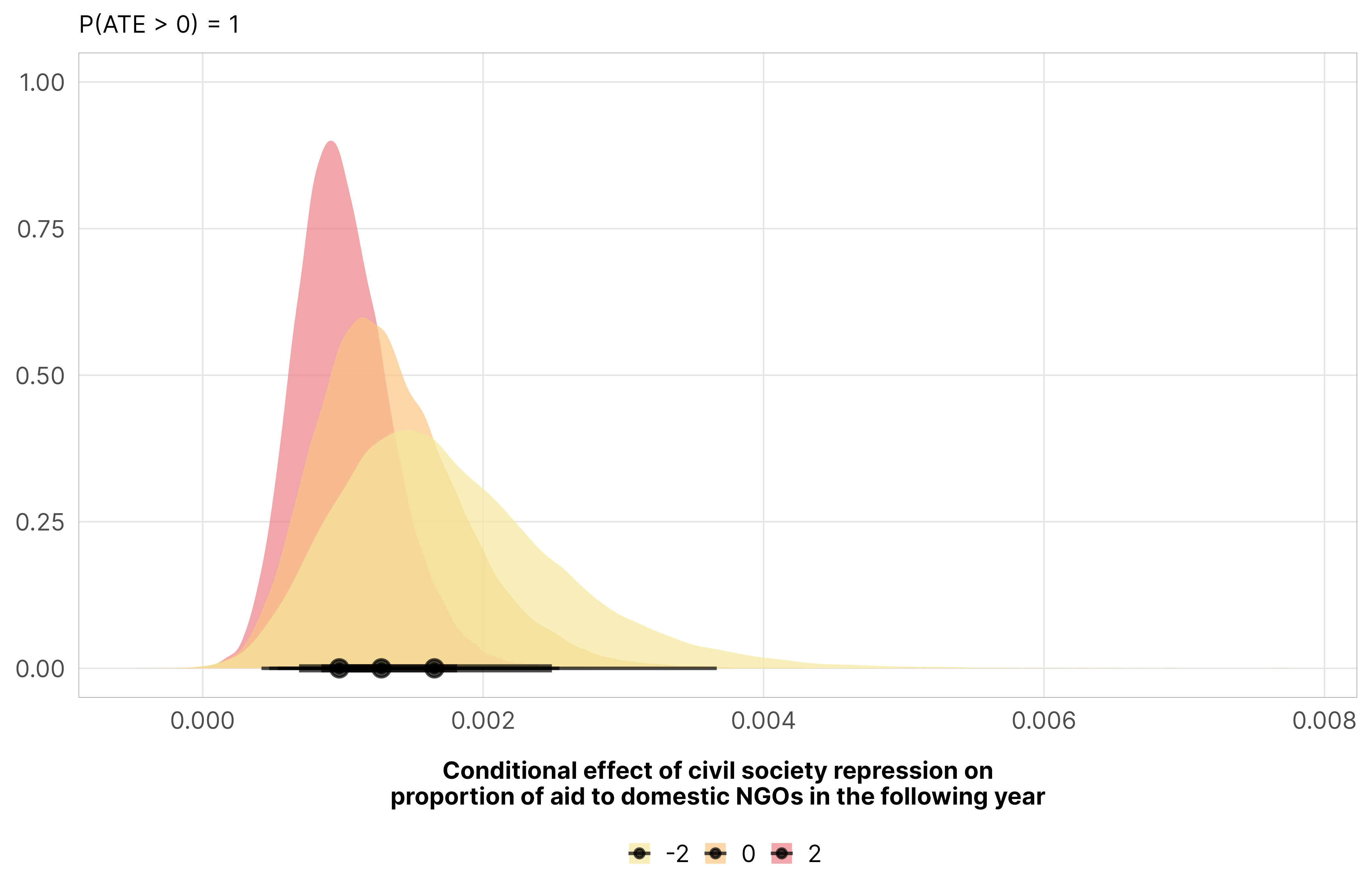
With civil society repression, there’s again a slightly different story. Worsening repression leads to a little more aid allocated to domestic NGOs, with a marginal effect of 0.13 percentage points (and a 100% probability that that’s positive).

Code

m_recip_outcome_repress_dom$model_50 %>% 
  epred_draws(newdata = datagrid(model = m_recip_outcome_repress_dom$model_50,
                                 year_c = 0,
                                 v2csreprss = seq(-4, 3, 0.25)),
              re_formula = NA)  %>% 
  ggplot(aes(x = v2csreprss, y = .epred)) +
  stat_lineribbon(color = clrs$Peach[7]) +
  scale_x_reverse() +
  scale_y_continuous(labels = label_percent()) +
  scale_fill_manual(values = clrs$Peach[1:3]) +
  guides(fill = "none") +
  labs(x = "Civil society repression", y = "Predicted proportion of\naid to domestic NGOs in the following year",
       caption = "**x-axis reversed**; lower values represent worse civil society repression") +
  theme_donors() +
  theme(plot.caption = element_markdown())

Code

mfx_recip_cfx_multiple_dom$repress %>% 
  select(v2csreprss, dydx, conf.low, conf.high)
##   v2csreprss      dydx conf.low conf.high
## 1         -2 -0.001653 -0.00367 -0.000535
## 2          0 -0.001275 -0.00254 -0.000474
## 3          2 -0.000974 -0.00177 -0.000419

Code

mfx_repress_p_direction_dom <- mfx_recip_cfx_multiple_dom$repress %>% 
  posteriordraws() %>% 
  filter(v2csreprss == 0) %>% 
  summarize(pd = sum(draw < 0) / n()) %>% 
  mutate(pd_short = round(pd, 2))

Code

mfx_recip_cfx_multiple_dom$repress %>% 
  posteriordraws() %>% 
  mutate(draw = -draw) %>% 
  pivot_longer(draw) %>% 
  ggplot(aes(x = value, fill = factor(v2csreprss))) +
  stat_halfeye(alpha = 0.7) +
  scale_x_continuous(labels = label_number(style_negative = "minus")) +
  scale_fill_manual(values = clrs$Sunset[c(1, 2, 4, 6, 7)]) +
  labs(x = "Conditional effect of civil society repression on\nproportion of aid to domestic NGOs in the following year", y = NULL,
       subtitle = glue("P(ATE > 0) = {pull(mfx_repress_p_direction_dom, pd_short)}"), fill = NULL) +
  theme_donors()

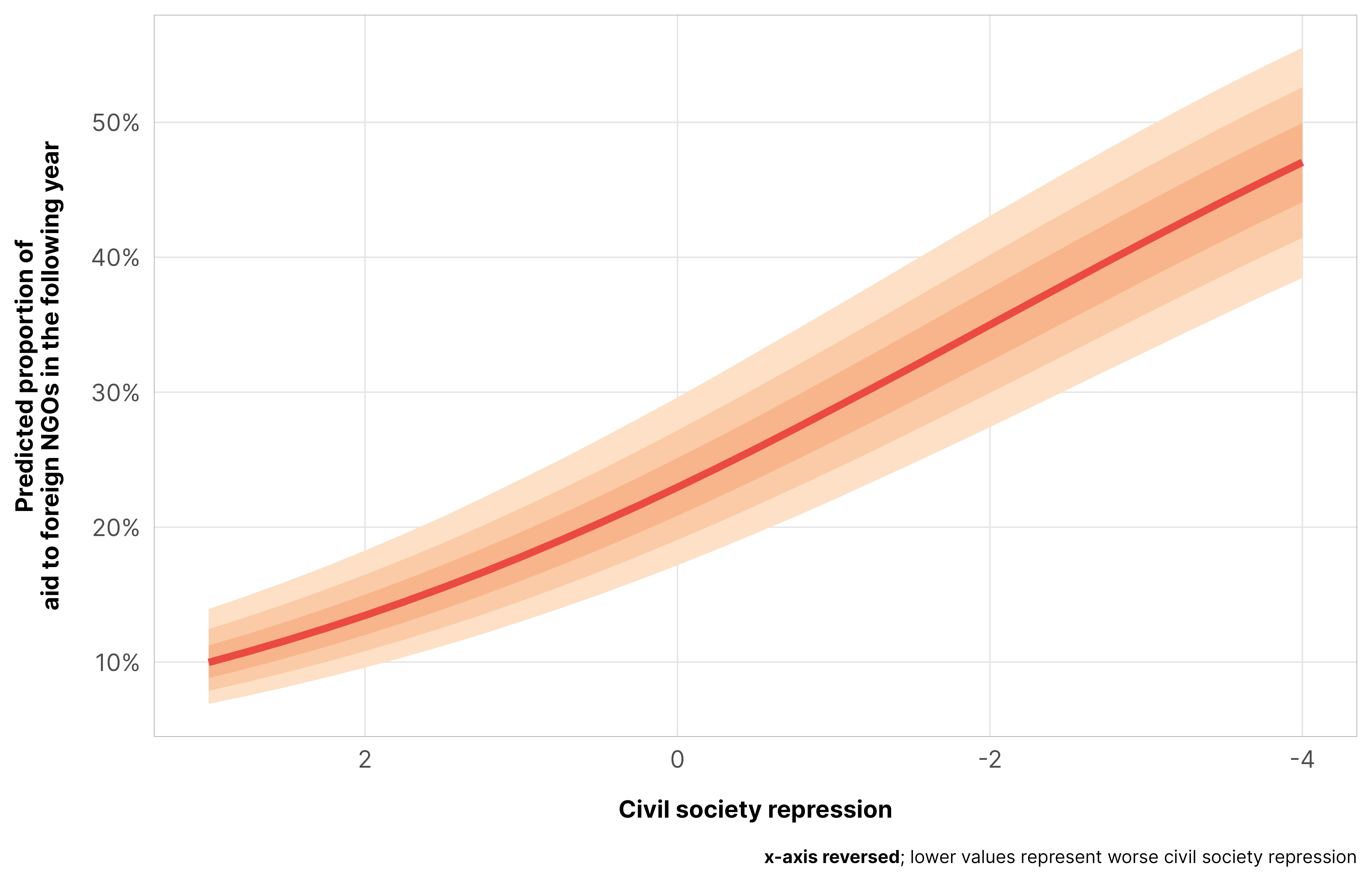
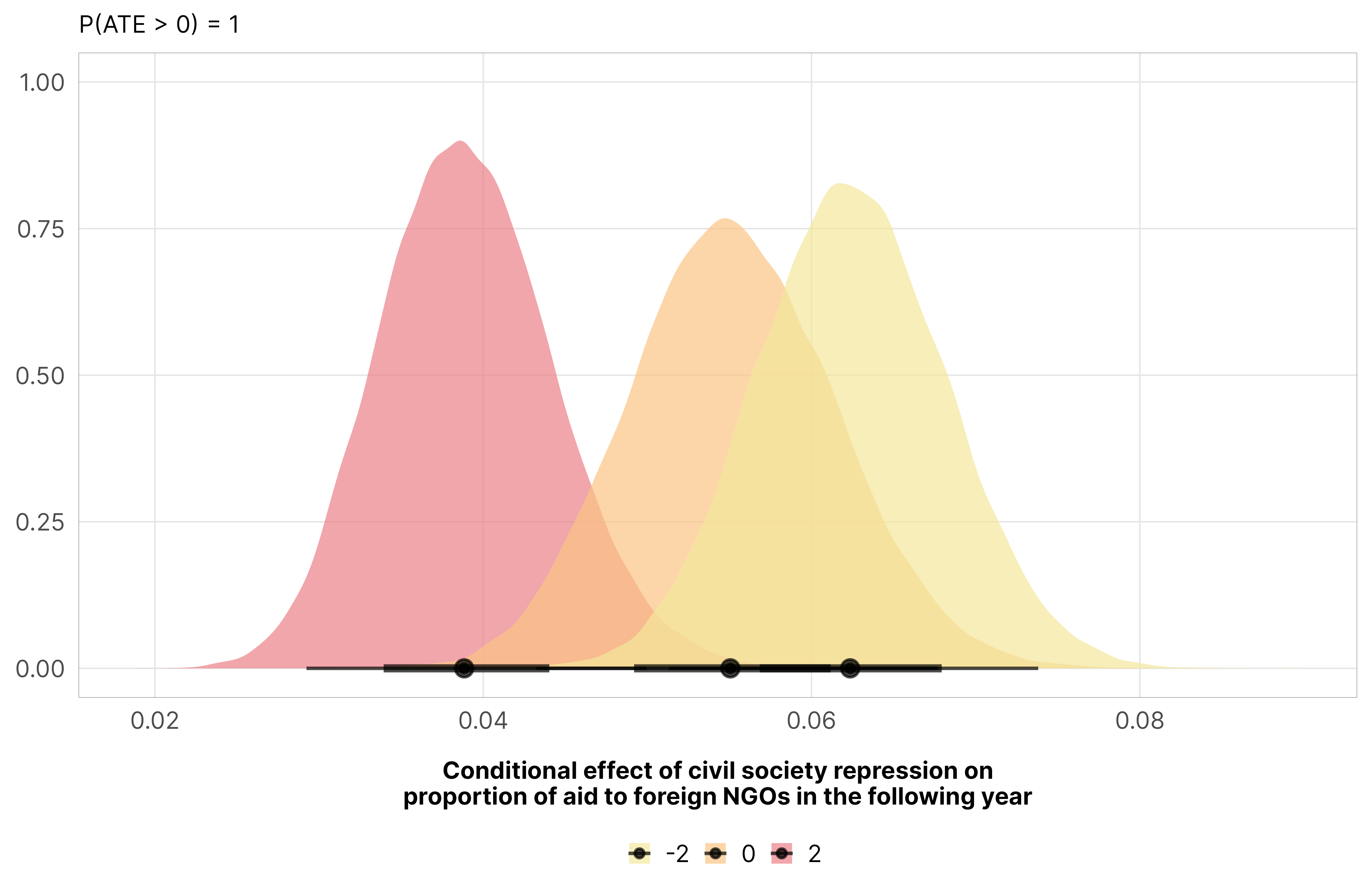
Even more striking, though, is USAID’s response with foreign NGO recipients. As civil society repression increases, WAY more aid is sent through foreign NGOs, with a marginal effect of 5.5 percentage points(!) (and a 100% probability of being positive).

Code

m_recip_outcome_repress_foreign$model_50 %>% 
  epred_draws(newdata = datagrid(model = m_recip_outcome_repress_foreign$model_50,
                                 year_c = 0,
                                 v2csreprss = seq(-4, 3, 0.25)),
              re_formula = NA)  %>% 
  ggplot(aes(x = v2csreprss, y = .epred)) +
  stat_lineribbon(color = clrs$Peach[7]) +
  scale_x_reverse() +
  scale_y_continuous(labels = label_percent()) +
  scale_fill_manual(values = clrs$Peach[1:3]) +
  guides(fill = "none") +
  labs(x = "Civil society repression", y = "Predicted proportion of\naid to foreign NGOs in the following year",
       caption = "**x-axis reversed**; lower values represent worse civil society repression") +
  theme_donors() +
  theme(plot.caption = element_markdown())

Code

mfx_recip_cfx_multiple_foreign$repress %>% 
  select(v2csreprss, dydx, conf.low, conf.high)
##   v2csreprss    dydx conf.low conf.high
## 1         -2 -0.0624  -0.0738   -0.0513
## 2          0 -0.0551  -0.0677   -0.0432
## 3          2 -0.0388  -0.0500   -0.0292

Code

mfx_repress_p_direction_foreign <- mfx_recip_cfx_multiple_foreign$repress %>% 
  posteriordraws() %>% 
  filter(v2csreprss == 0) %>% 
  summarize(pd = sum(draw < 0) / n()) %>% 
  mutate(pd_short = round(pd, 2))

Code

mfx_recip_cfx_multiple_foreign$repress %>% 
  posteriordraws() %>% 
  mutate(draw = -draw) %>% 
  pivot_longer(draw) %>% 
  ggplot(aes(x = value, fill = factor(v2csreprss))) +
  stat_halfeye(alpha = 0.7) +
  scale_x_continuous(labels = label_number(style_negative = "minus")) +
  scale_fill_manual(values = clrs$Sunset[c(1, 2, 4, 6, 7)]) +
  labs(x = "Conditional effect of civil society repression on\nproportion of aid to foreign NGOs in the following year", y = NULL,
       subtitle = glue("P(ATE > 0) = {pull(mfx_repress_p_direction_foreign, pd_short)}"), fill = NULL) +
  theme_donors()

Combined plots

Predictions: Proportion of aid to domestic NGOs

Code

ci_cols <- c("grey70", "grey45", "grey20")

p1 <- m_recip_outcome_total_dom$model %>% 
  epred_draws(newdata = datagrid(model = m_recip_outcome_total_dom$model,
                                 year_c = 0,
                                 barriers_total = seq(0, 10, 1)),
              re_formula = NA) %>% 
  ggplot(aes(x = barriers_total, y = .epred)) +
  stat_lineribbon(aes(color = "Posterior median"), 
                  alpha = 0.6, point_interval = median_hdci) +
  scale_x_continuous(breaks = seq(0, 10, by = 2)) +
  scale_y_continuous(labels = label_percent(accuracy = 1)) +
  scale_color_manual(
    values = clrs$PurpOr[7],
    guide = guide_legend(order = 1, 
                         override.aes = list(fill = NA, alpha = 1, color = "black"))
  ) +
  scale_fill_manual(
    values = clrs$PurpOr[c(1, 3, 5)], 
    labels = function(x) label_percent()(as.numeric(x)),
    guide = guide_legend(order = 2, 
                         override.aes = list(color = NA, fill = ci_cols))
  ) +
  labs(x = NULL, y = NULL, color = NULL, fill = "Credible interval (HPDI):") +
  coord_cartesian(ylim = c(0, 0.085)) +
  facet_wrap(vars("Total barriers")) +
  theme_donors() + 
  theme(legend.margin = margin(l = 7.5, r = 7.5))

p2 <- m_recip_outcome_advocacy_dom$model %>% 
  epred_draws(newdata = datagrid(model = m_recip_outcome_advocacy_dom$model,
                                 year_c = 0,
                                 advocacy = seq(0, 2, 1)),
              re_formula = NA) %>% 
  ggplot(aes(x = advocacy, y = .epred)) +
  stat_lineribbon(aes(color = "Posterior median"), 
                  alpha = 0.6, point_interval = median_hdci) +
  scale_x_continuous(breaks = 0:2) +
  scale_y_continuous(labels = label_percent(accuracy = 1)) +
  scale_color_manual(
    values = clrs$Teal[7],
    guide = guide_legend(order = 1, 
                         override.aes = list(fill = NA, alpha = 1, color = "black"))
  ) +
  scale_fill_manual(
    values = clrs$Teal[c(1, 3, 5)], 
    labels = function(x) label_percent()(as.numeric(x)),
    guide = guide_legend(order = 2, 
                         override.aes = list(color = NA, fill = ci_cols))
  ) +
  labs(x = NULL, y = NULL, color = NULL, fill = "Credible interval (HPDI):") +
  coord_cartesian(ylim = c(0, 0.085)) +
  facet_wrap(vars("Barriers to advocacy")) +
  theme_donors() + 
  theme(legend.margin = margin(l = 7.5, r = 7.5))

p3 <- m_recip_outcome_entry_dom$model %>% 
  epred_draws(newdata = datagrid(model = m_recip_outcome_entry_dom$model,
                                 year_c = 0,
                                 entry = seq(0, 3, 1)),
              re_formula = NA) %>% 
  ggplot(aes(x = entry, y = .epred)) +
  stat_lineribbon(aes(color = "Posterior median"), 
                  alpha = 0.6, point_interval = median_hdci) +
  scale_x_continuous(breaks = 0:3) +
  scale_y_continuous(labels = label_percent(accuracy = 1)) +
  scale_color_manual(
    values = clrs$Emrld[7],
    guide = guide_legend(order = 1, 
                         override.aes = list(fill = NA, alpha = 1, color = "black"))
  ) +
  scale_fill_manual(
    values = clrs$Emrld[c(1, 3, 5)], 
    labels = function(x) label_percent()(as.numeric(x)),
    guide = guide_legend(order = 2, 
                         override.aes = list(color = NA, fill = ci_cols))
  ) +
  labs(x = NULL, y = NULL, color = NULL, fill = "Credible interval (HPDI):") +
  coord_cartesian(ylim = c(0, 0.085)) +
  facet_wrap(vars("Barriers to entry")) +
  theme_donors() + 
  theme(legend.margin = margin(l = 7.5, r = 7.5))

p4 <- m_recip_outcome_funding_dom$model %>% 
  epred_draws(newdata = datagrid(model = m_recip_outcome_funding_dom$model,
                                 year_c = 0,
                                 funding = seq(0, 4, 1)),
              re_formula = NA) %>% 
  ggplot(aes(x = funding, y = .epred)) +
  stat_lineribbon(aes(color = "Posterior median"), 
                  alpha = 0.6, point_interval = median_hdci) +
  scale_x_continuous(breaks = 0:4) +
  scale_y_continuous(labels = label_percent(accuracy = 1)) +
  scale_color_manual(
    values = clrs$Peach[7],
    guide = guide_legend(order = 1, 
                         override.aes = list(fill = NA, alpha = 1, color = "black"))
  ) +
  scale_fill_manual(
    values = clrs$Peach[c(1, 3, 5)], 
    labels = function(x) label_percent()(as.numeric(x)),
    guide = guide_legend(order = 2, 
                         override.aes = list(color = NA, fill = ci_cols))
  ) +
  labs(x = NULL, y = NULL, color = NULL, fill = "Credible interval (HPDI):") +
  coord_cartesian(ylim = c(0, 0.085)) +
  facet_wrap(vars("Barriers to funding")) +
  theme_donors() + 
  theme(legend.margin = margin(l = 7.5, r = 7.5))

Code

# Put the shared y-axis label in a separate plot and add it to the combined plot
# https://stackoverflow.com/a/66778622/120898
p_lab <- ggplot() + 
  annotate(geom = "text", x = 1, y = 1, angle = 90, size = 3.3, fontface = "bold",
           label = "Predicted proportion of\naid to domestic NGOs in the following year") +
  coord_cartesian(clip = "off") +
  theme_void()

(p_lab | 
    ((p1 | p2) / (p3 | p4) + 
       plot_layout(guides = "collect") + 
       plot_annotation(theme = theme(legend.position = "bottom")))) + 
  plot_layout(widths = c(0.05, 1))

The effect of de jure anti-NGO legal barriers on the predicted proportion of USAID aid allocated to domestic NGOs in a typical country

Code

p1 <- m_recip_outcome_ccsi_dom$model_50 %>% 
  epred_draws(newdata = datagrid(model = m_recip_outcome_ccsi_dom$model_50,
                                 year_c = 0,
                                 v2xcs_ccsi = seq(0, 1, 0.1)),
              re_formula = NA) %>% 
  ggplot(aes(x = v2xcs_ccsi, y = .epred)) +
  stat_lineribbon(aes(color = "Posterior median"), 
                  alpha = 0.6, point_interval = median_hdci) +
  scale_x_reverse(breaks = seq(0, 1, by = 0.25)) +
  scale_y_continuous(labels = label_percent(accuracy = 1)) +
  scale_color_manual(
    values = clrs$Sunset[4],
    guide = guide_legend(order = 1, 
                         override.aes = list(fill = NA, alpha = 1, color = "black"))
  ) +
  scale_fill_manual(
    values = clrs$Sunset[c(1, 2, 3)], 
    labels = function(x) label_percent()(as.numeric(x)),
    guide = guide_legend(order = 2, 
                         override.aes = list(color = NA, fill = ci_cols))
  ) +
  labs(x = NULL, y = NULL, color = NULL, fill = "Credible interval (HPDI):") +
  coord_cartesian(ylim = c(0, 0.04)) +
  facet_wrap(vars("Worsening core civil society index")) +
  theme_donors() +
  theme(legend.margin = margin(l = 7.5, r = 7.5))

p2 <- m_recip_outcome_repress_dom$model_50 %>% 
  epred_draws(newdata = datagrid(model = m_recip_outcome_repress_dom$model_50,
                                 year_c = 0,
                                 v2csreprss = seq(-4, 3, 0.25)),
              re_formula = NA) %>% 
  ggplot(aes(x = v2csreprss, y = .epred)) +
  stat_lineribbon(aes(color = "Posterior median"), 
                  alpha = 0.6, point_interval = median_hdci) +
  scale_x_reverse(labels = label_number(style_negative = "minus")) +
  scale_y_continuous(labels = label_percent(accuracy = 1)) +
  scale_color_manual(
    values = clrs$Sunset[7],
    guide = guide_legend(order = 1, 
                         override.aes = list(fill = NA, alpha = 1, color = "black"))
  ) +
  scale_fill_manual(
    values = clrs$Sunset[c(4, 5, 6)], 
    labels = function(x) label_percent()(as.numeric(x)),
    guide = guide_legend(order = 2, 
                         override.aes = list(color = NA, fill = ci_cols))
  ) +
  labs(x = NULL, y = NULL, color = NULL, fill = "Credible interval (HPDI):",
       caption = "**x-axis reversed**; lower values represent worse respect for and repression of civil society") +
  coord_cartesian(ylim = c(0, 0.04)) +
  facet_wrap(vars("Worsening civil society repression")) +
  theme_donors() +
  theme(legend.margin = margin(l = 7.5, r = 7.5),
        plot.caption = element_markdown())

p_lab <- ggplot() + 
  annotate(geom = "text", x = 1, y = 1, angle = 90, size = 3.3, fontface = "bold",
           label = "Predicted proportion of\naid to domestic NGOs in the following year") +
  coord_cartesian(clip = "off") +
  theme_void()

(p_lab | 
    ((p1 | p2) + 
       plot_layout(guides = "collect") + 
       plot_annotation(theme = theme(legend.position = "bottom")))) + 
  plot_layout(widths = c(0.05, 1))

The effect of the de facto civil society legal environment on the predicted proportion of USAID aid channeled to domestic NGOs aid in a typical country

Conditional marginal effects: Proportion of aid to domestic NGOs

Code

mfx_total_stats_dom <- mfx_recip_cfx_single_dom$total %>% 
  posteriordraws() %>% 
  summarize(pd = sum(draw < 0) / n(),
            mad = mad(draw),
            med_hdci = median_hdci(draw)) %>% 
  unnest(med_hdci) %>% 
  mutate(pd_short = round(pd, 2))

mfx_advocacy_stats_dom <- mfx_recip_cfx_single_dom$advocacy %>% 
  posteriordraws() %>% 
  summarize(pd = sum(draw < 0) / n(),
            mad = mad(draw),
            med_hdci = median_hdci(draw)) %>% 
  unnest(med_hdci) %>% 
  mutate(pd_short = round(pd, 2))

mfx_entry_stats_dom <- mfx_recip_cfx_single_dom$entry %>% 
  posteriordraws() %>% 
  summarize(pd = sum(draw < 0) / n(),
            mad = mad(draw),
            med_hdci = median_hdci(draw)) %>% 
  unnest(med_hdci) %>% 
  mutate(pd_short = round(pd, 2))

mfx_funding_stats_dom <- mfx_recip_cfx_single_dom$funding %>% 
  posteriordraws() %>% 
  summarize(pd = sum(draw < 0) / n(),
            mad = mad(draw),
            med_hdci = median_hdci(draw)) %>% 
  unnest(med_hdci) %>% 
  mutate(pd_short = round(pd, 2))

mfx_ccsi_stats_dom <- mfx_recip_cfx_single_dom$ccsi %>% 
  posteriordraws() %>% 
  summarize(pd = sum(draw < 0) / n(),
            mad = mad(draw),
            med_hdci = median_hdci(draw)) %>% 
  unnest(med_hdci) %>% 
  mutate(pd_short = round(pd, 2))

mfx_repress_stats_dom <- mfx_recip_cfx_single_dom$repress %>% 
  posteriordraws() %>% 
  summarize(pd = sum(draw < 0) / n(),
            mad = mad(draw),
            med_hdci = median_hdci(draw)) %>% 
  unnest(med_hdci) %>% 
  mutate(pd_short = round(pd, 2))

Code

p1 <- mfx_recip_cfx_single_dom$total %>% 
  posteriordraws() %>% 
  ggplot(aes(x = draw)) +
  stat_halfeye(aes(fill_ramp = after_stat(x < 0)),
               fill = clrs$PurpOr[6], .width = c(0.8, 0.95),
               point_interval = median_hdci) +
  geom_vline(xintercept = 0, linewidth = 0.25) +
  annotate(geom = "richtext", label = glue("P(ATE > 0) = {1 - pull(mfx_total_stats_dom, pd_short)}"),
           x = Inf, y = Inf, hjust = 1, vjust = 1, size = 3,
           label.color = NA, label.margin = unit(rep(0.5, 4), "lines")) +
  scale_x_continuous(labels = label_number(scale = 100, suffix = " pp.",
                                           style_negative = "minus")) +
  scale_fill_ramp_discrete(from = clrs$PurpOr[4], guide = "none") +
  labs(x = NULL, y = NULL, fill = NULL) +
  facet_wrap(vars("One additional barrier of any type")) +
  theme_donors() +
  theme(axis.text.y = element_blank())

p2 <- mfx_recip_cfx_single_dom$advocacy %>% 
  posteriordraws() %>% 
  ggplot(aes(x = draw)) +
  stat_halfeye(aes(fill_ramp = after_stat(x < 0)),
               fill = clrs$Teal[4], .width = c(0.8, 0.95),
               point_interval = median_hdci) +
  geom_vline(xintercept = 0, linewidth = 0.25) +
  annotate(geom = "richtext", label = glue("P(ATE < 0) = {pull(mfx_advocacy_stats_dom, pd_short)}"),
           x = Inf, y = Inf, hjust = 1, vjust = 1, size = 3,
           label.color = NA, label.margin = unit(rep(0.5, 4), "lines")) +
  scale_x_continuous(labels = label_number(scale = 100, suffix = " pp.",
                                           style_negative = "minus")) +
  scale_fill_ramp_discrete(from = clrs$Teal[6], guide = "none") +
  labs(x = NULL, y = NULL, fill = NULL) +
  facet_wrap(vars("One additional barrier to advocacy")) +
  theme_donors() +
  theme(axis.text.y = element_blank())

p3 <- mfx_recip_cfx_single_dom$entry %>% 
  posteriordraws() %>% 
  ggplot(aes(x = draw)) +
  stat_halfeye(aes(fill_ramp = after_stat(x < 0)),
               fill = clrs$Emrld[4], .width = c(0.8, 0.95),
               point_interval = median_hdci) +
  geom_vline(xintercept = 0, linewidth = 0.25) +
  annotate(geom = "richtext", label = glue("P(ATE > 0) = {1 - pull(mfx_entry_stats_dom, pd_short)}"),
           x = Inf, y = Inf, hjust = 1, vjust = 1, size = 3,
           label.color = NA, label.margin = unit(rep(0.5, 4), "lines")) +
  scale_x_continuous(labels = label_number(scale = 100, suffix = " pp.",
                                           style_negative = "minus")) +
  scale_fill_ramp_discrete(from = clrs$Emrld[6], guide = "none") +
  labs(x = NULL, y = NULL, fill = NULL) +
  facet_wrap(vars("One additional barrier to entry")) +
  theme_donors() +
  theme(axis.text.y = element_blank())

p4 <- mfx_recip_cfx_single_dom$funding %>% 
  posteriordraws() %>% 
  ggplot(aes(x = draw)) +
  stat_halfeye(aes(fill_ramp = after_stat(x < 0)),
               fill = clrs$Peach[6], .width = c(0.8, 0.95),
               point_interval = median_hdci) +
  geom_vline(xintercept = 0, linewidth = 0.25) +
  annotate(geom = "richtext", label = glue("P(ATE > 0) = {1 - pull(mfx_funding_stats_dom, pd_short)}"),
           x = Inf, y = Inf, hjust = 1, vjust = 1, size = 3,
           label.color = NA, label.margin = unit(rep(0.5, 4), "lines")) +
  scale_x_continuous(labels = label_number(scale = 100, suffix = " pp.",
                                           style_negative = "minus")) +
  scale_fill_ramp_discrete(from = clrs$Peach[4], guide = "none") +
  labs(x = NULL, y = NULL, fill = NULL) +
  facet_wrap(vars("One additional barrier to funding")) +
  theme_donors() +
  theme(axis.text.y = element_blank())

Code

p_lab <- ggplot() + 
  annotate(geom = "text", x = 1, y = 1, size = 3.3, fontface = "bold",
           label = "Conditional effect of treatment on proportion\nof aid to domestic NGOs in the following year") +
  coord_cartesian(clip = "off") +
  theme_void()

(((p1 | p2) / (p3 | p4)) / p_lab) + 
  plot_layout(heights = c(1, 1, 0.2)) +
  plot_annotation(caption = "Point shows median value;\nthick bar = 80% credible interval; thin bar = 95% credible interval",
                  theme = theme(plot.caption = element_text(family = "Inter")))

The effect of one additional de jure anti-NGO legal barrier on the proportion of USAID aid allocated to domestic NGOs in a typical country

Code

p1 <- mfx_recip_cfx_single_dom$ccsi %>% 
  posteriordraws() %>% 
  mutate(draw = -draw / 10) %>% 
  ggplot(aes(x = draw)) +
  stat_halfeye(aes(fill_ramp = after_stat(x < 0)),
               fill = clrs$Sunset[4], .width = c(0.8, 0.95),
               point_interval = median_hdci) +
  geom_vline(xintercept = 0, linewidth = 0.25) +
  annotate(geom = "richtext", label = glue("P(ATE < 0) = {1 - pull(mfx_ccsi_stats_dom, pd_short)}"),
           x = Inf, y = Inf, hjust = 1, vjust = 1, size = 3,
           label.color = NA, label.margin = unit(rep(0.5, 4), "lines")) +
  scale_x_continuous(labels = label_number(scale = 100, suffix = " pp.",
                                           style_negative = "minus")) +
  scale_fill_ramp_discrete(from = clrs$Sunset[3], guide = "none") +
  labs(x = NULL, y = NULL, fill = NULL) +
  facet_wrap(vars("A 0.1 unit decrease (worsening) in\nthe core civil society index")) +
  theme_donors() +
  theme(axis.text.y = element_blank())

p2 <- mfx_recip_cfx_single_dom$repress %>% 
  posteriordraws() %>% 
  mutate(draw = -draw) %>% 
  ggplot(aes(x = draw)) +
  stat_halfeye(aes(fill_ramp = after_stat(x > 0)),
               fill = clrs$Sunset[6], .width = c(0.8, 0.95),
               point_interval = median_hdci) +
  geom_vline(xintercept = 0, linewidth = 0.25) +
  annotate(geom = "richtext", label = glue("P(ATE > 0) = {pull(mfx_repress_stats_dom, pd_short)}"),
           x = Inf, y = Inf, hjust = 1, vjust = 1, size = 3,
           label.color = NA, label.margin = unit(rep(0.5, 4), "lines")) +
  scale_x_continuous(labels = label_number(scale = 100, suffix = " pp.",
                                           style_negative = "minus")) +
  scale_fill_ramp_discrete(from = clrs$Sunset[3], guide = "none") +
  labs(x = NULL, y = NULL, fill = NULL) +
  facet_wrap(vars("A 1 unit increase (improvement) in\nthe civil society repression score")) +
  theme_donors() +
  theme(axis.text.y = element_blank())

p_lab <- ggplot() + 
  annotate(geom = "text", x = 1, y = 1, size = 3.3, fontface = "bold",
           label = "Conditional effect of treatment on proportion\nof aid to domestic NGOs in the following year") +
  coord_cartesian(clip = "off") +
  theme_void()

((p1 | p2) / p_lab) + 
  plot_layout(heights = c(1, 0.18)) +
  plot_annotation(caption = "Point shows median value;\nthick bar = 80% credible interval; thin bar = 95% credible interval",
                  theme = theme(plot.caption = element_text(family = "Inter")))

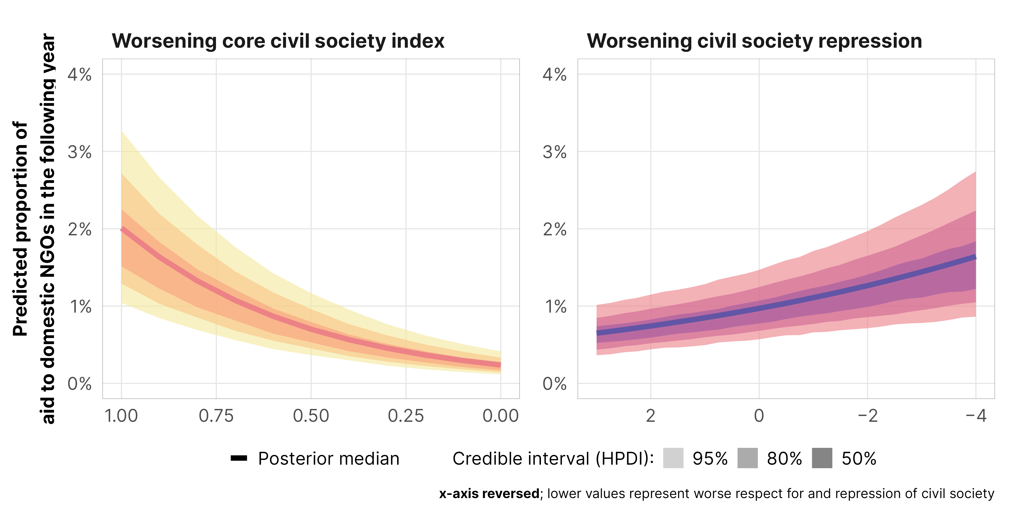
The effect of changes in the de facto civil society legal environment on the predicted proportion of USAID aid allocated to domestic NGOs in a typical country

Predictions: Proportion of aid to foreign NGOs

Code

ci_cols <- c("grey70", "grey45", "grey20")

p1 <- m_recip_outcome_total_foreign$model %>% 
  epred_draws(newdata = datagrid(model = m_recip_outcome_total_foreign$model,
                                 year_c = 0,
                                 barriers_total = seq(0, 10, 1)),
              re_formula = NA) %>% 
  ggplot(aes(x = barriers_total, y = .epred)) +
  stat_lineribbon(aes(color = "Posterior median"), 
                  alpha = 0.6, point_interval = median_hdci) +
  scale_x_continuous(breaks = seq(0, 10, by = 2)) +
  scale_y_continuous(labels = label_percent(accuracy = 1)) +
  scale_color_manual(
    values = clrs$PurpOr[7],
    guide = guide_legend(order = 1, 
                         override.aes = list(fill = NA, alpha = 1, color = "black"))
  ) +
  scale_fill_manual(
    values = clrs$PurpOr[c(1, 3, 5)], 
    labels = function(x) label_percent()(as.numeric(x)),
    guide = guide_legend(order = 2, 
                         override.aes = list(color = NA, fill = ci_cols))
  ) +
  labs(x = NULL, y = NULL, color = NULL, fill = "Credible interval (HPDI):") +
  coord_cartesian(ylim = c(0.15, 0.42)) +
  facet_wrap(vars("Total barriers")) +
  theme_donors() + 
  theme(legend.margin = margin(l = 7.5, r = 7.5))

p2 <- m_recip_outcome_advocacy_foreign$model %>% 
  epred_draws(newdata = datagrid(model = m_recip_outcome_advocacy_foreign$model,
                                 year_c = 0,
                                 advocacy = seq(0, 2, 1)),
              re_formula = NA) %>% 
  ggplot(aes(x = advocacy, y = .epred)) +
  stat_lineribbon(aes(color = "Posterior median"), 
                  alpha = 0.6, point_interval = median_hdci) +
  scale_x_continuous(breaks = 0:2) +
  scale_y_continuous(labels = label_percent(accuracy = 1)) +
  scale_color_manual(
    values = clrs$Teal[7],
    guide = guide_legend(order = 1, 
                         override.aes = list(fill = NA, alpha = 1, color = "black"))
  ) +
  scale_fill_manual(
    values = clrs$Teal[c(1, 3, 5)], 
    labels = function(x) label_percent()(as.numeric(x)),
    guide = guide_legend(order = 2, 
                         override.aes = list(color = NA, fill = ci_cols))
  ) +
  labs(x = NULL, y = NULL, color = NULL, fill = "Credible interval (HPDI):") +
  coord_cartesian(ylim = c(0.15, 0.42)) +
  facet_wrap(vars("Barriers to advocacy")) +
  theme_donors() + 
  theme(legend.margin = margin(l = 7.5, r = 7.5))

p3 <- m_recip_outcome_entry_foreign$model %>% 
  epred_draws(newdata = datagrid(model = m_recip_outcome_entry_foreign$model,
                                 year_c = 0,
                                 entry = seq(0, 3, 1)),
              re_formula = NA) %>% 
  ggplot(aes(x = entry, y = .epred)) +
  stat_lineribbon(aes(color = "Posterior median"), 
                  alpha = 0.6, point_interval = median_hdci) +
  scale_x_continuous(breaks = 0:3) +
  scale_y_continuous(labels = label_percent(accuracy = 1)) +
  scale_color_manual(
    values = clrs$Emrld[7],
    guide = guide_legend(order = 1, 
                         override.aes = list(fill = NA, alpha = 1, color = "black"))
  ) +
  scale_fill_manual(
    values = clrs$Emrld[c(1, 3, 5)], 
    labels = function(x) label_percent()(as.numeric(x)),
    guide = guide_legend(order = 2, 
                         override.aes = list(color = NA, fill = ci_cols))
  ) +
  labs(x = NULL, y = NULL, color = NULL, fill = "Credible interval (HPDI):") +
  coord_cartesian(ylim = c(0.15, 0.42)) +
  facet_wrap(vars("Barriers to entry")) +
  theme_donors() + 
  theme(legend.margin = margin(l = 7.5, r = 7.5))

p4 <- m_recip_outcome_funding_foreign$model %>% 
  epred_draws(newdata = datagrid(model = m_recip_outcome_funding_foreign$model,
                                 year_c = 0,
                                 funding = seq(0, 4, 1)),
              re_formula = NA) %>% 
  ggplot(aes(x = funding, y = .epred)) +
  stat_lineribbon(aes(color = "Posterior median"), 
                  alpha = 0.6, point_interval = median_hdci) +
  scale_x_continuous(breaks = 0:4) +
  scale_y_continuous(labels = label_percent(accuracy = 1)) +
  scale_color_manual(
    values = clrs$Peach[7],
    guide = guide_legend(order = 1, 
                         override.aes = list(fill = NA, alpha = 1, color = "black"))
  ) +
  scale_fill_manual(
    values = clrs$Peach[c(1, 3, 5)], 
    labels = function(x) label_percent()(as.numeric(x)),
    guide = guide_legend(order = 2, 
                         override.aes = list(color = NA, fill = ci_cols))
  ) +
  labs(x = NULL, y = NULL, color = NULL, fill = "Credible interval (HPDI):") +
  coord_cartesian(ylim = c(0.15, 0.42)) +
  facet_wrap(vars("Barriers to funding")) +
  theme_donors() + 
  theme(legend.margin = margin(l = 7.5, r = 7.5))

Code

# Put the shared y-axis label in a separate plot and add it to the combined plot
# https://stackoverflow.com/a/66778622/120898
p_lab <- ggplot() + 
  annotate(geom = "text", x = 1, y = 1, angle = 90, size = 3.3, fontface = "bold",
           label = "Predicted proportion of\naid to foreign NGOs in the following year") +
  coord_cartesian(clip = "off") +
  theme_void()

(p_lab | 
    ((p1 | p2) / (p3 | p4) + 
       plot_layout(guides = "collect") + 
       plot_annotation(theme = theme(legend.position = "bottom")))) + 
  plot_layout(widths = c(0.05, 1))

The effect of de jure anti-NGO legal barriers on the predicted proportion of USAID aid allocated to foreign NGOs in a typical country

Code

p1 <- m_recip_outcome_ccsi_foreign$model_50 %>% 
  epred_draws(newdata = datagrid(model = m_recip_outcome_ccsi_foreign$model_50,
                                 year_c = 0,
                                 v2xcs_ccsi = seq(0, 1, 0.1)),
              re_formula = NA) %>% 
  ggplot(aes(x = v2xcs_ccsi, y = .epred)) +
  stat_lineribbon(aes(color = "Posterior median"), 
                  alpha = 0.6, point_interval = median_hdci) +
  scale_x_reverse(breaks = seq(0, 1, by = 0.25)) +
  scale_y_continuous(labels = label_percent(accuracy = 1)) +
  scale_color_manual(
    values = clrs$Sunset[4],
    guide = guide_legend(order = 1, 
                         override.aes = list(fill = NA, alpha = 1, color = "black"))
  ) +
  scale_fill_manual(
    values = clrs$Sunset[c(1, 2, 3)], 
    labels = function(x) label_percent()(as.numeric(x)),
    guide = guide_legend(order = 2, 
                         override.aes = list(color = NA, fill = ci_cols))
  ) +
  labs(x = NULL, y = NULL, color = NULL, fill = "Credible interval (HPDI):") +
  coord_cartesian(ylim = c(0, 0.6)) +
  facet_wrap(vars("Worsening core civil society index")) +
  theme_donors() +
  theme(legend.margin = margin(l = 7.5, r = 7.5))

p2 <- m_recip_outcome_repress_foreign$model_50 %>% 
  epred_draws(newdata = datagrid(model = m_recip_outcome_repress_foreign$model_50,
                                 year_c = 0,
                                 v2csreprss = seq(-4, 3, 0.25)),
              re_formula = NA) %>% 
  ggplot(aes(x = v2csreprss, y = .epred)) +
  stat_lineribbon(aes(color = "Posterior median"), 
                  alpha = 0.6, point_interval = median_hdci) +
  scale_x_reverse(labels = label_number(style_negative = "minus")) +
  scale_y_continuous(labels = label_percent(accuracy = 1)) +
  scale_color_manual(
    values = clrs$Sunset[7],
    guide = guide_legend(order = 1, 
                         override.aes = list(fill = NA, alpha = 1, color = "black"))
  ) +
  scale_fill_manual(
    values = clrs$Sunset[c(4, 5, 6)], 
    labels = function(x) label_percent()(as.numeric(x)),
    guide = guide_legend(order = 2, 
                         override.aes = list(color = NA, fill = ci_cols))
  ) +
  labs(x = NULL, y = NULL, color = NULL, fill = "Credible interval (HPDI):",
       caption = "**x-axis reversed**; lower values represent worse respect for and repression of civil society") +
  coord_cartesian(ylim = c(0, 0.6)) +
  facet_wrap(vars("Worsening civil society repression")) +
  theme_donors() +
  theme(legend.margin = margin(l = 7.5, r = 7.5),
        plot.caption = element_markdown())

p_lab <- ggplot() + 
  annotate(geom = "text", x = 1, y = 1, angle = 90, size = 3.3, fontface = "bold",
           label = "Predicted proportion of\naid to foreign NGOs in the following year") +
  coord_cartesian(clip = "off") +
  theme_void()

(p_lab | 
    ((p1 | p2) + 
       plot_layout(guides = "collect") + 
       plot_annotation(theme = theme(legend.position = "bottom")))) + 
  plot_layout(widths = c(0.05, 1))

The effect of the de facto civil society legal environment on the predicted proportion of USAID aid channeled to foreign NGOs aid in a typical country

Conditional marginal effects: Proportion of aid to foreign NGOs

Code

mfx_total_stats_foreign <- mfx_recip_cfx_single_foreign$total %>% 
  posteriordraws() %>% 
  summarize(pd = sum(draw < 0) / n(),
            mad = mad(draw),
            med_hdci = median_hdci(draw)) %>% 
  unnest(med_hdci) %>% 
  mutate(pd_short = round(pd, 2))

mfx_advocacy_stats_foreign <- mfx_recip_cfx_single_foreign$advocacy %>% 
  posteriordraws() %>% 
  summarize(pd = sum(draw < 0) / n(),
            mad = mad(draw),
            med_hdci = median_hdci(draw)) %>% 
  unnest(med_hdci) %>% 
  mutate(pd_short = round(pd, 2))

mfx_entry_stats_foreign <- mfx_recip_cfx_single_foreign$entry %>% 
  posteriordraws() %>% 
  summarize(pd = sum(draw < 0) / n(),
            mad = mad(draw),
            med_hdci = median_hdci(draw)) %>% 
  unnest(med_hdci) %>% 
  mutate(pd_short = round(pd, 2))

mfx_funding_stats_foreign <- mfx_recip_cfx_single_foreign$funding %>% 
  posteriordraws() %>% 
  summarize(pd = sum(draw < 0) / n(),
            mad = mad(draw),
            med_hdci = median_hdci(draw)) %>% 
  unnest(med_hdci) %>% 
  mutate(pd_short = round(pd, 2))

mfx_ccsi_stats_foreign <- mfx_recip_cfx_single_foreign$ccsi %>% 
  posteriordraws() %>% 
  summarize(pd = sum(draw < 0) / n(),
            mad = mad(draw),
            med_hdci = median_hdci(draw)) %>% 
  unnest(med_hdci) %>% 
  mutate(pd_short = round(pd, 2))

mfx_repress_stats_foreign <- mfx_recip_cfx_single_foreign$repress %>% 
  posteriordraws() %>% 
  summarize(pd = sum(draw < 0) / n(),
            mad = mad(draw),
            med_hdci = median_hdci(draw)) %>% 
  unnest(med_hdci) %>% 
  mutate(pd_short = round(pd, 2))

Code

p1 <- mfx_recip_cfx_single_foreign$total %>% 
  posteriordraws() %>% 
  ggplot(aes(x = draw)) +
  stat_halfeye(aes(fill_ramp = after_stat(x < 0)),
               fill = clrs$PurpOr[6], .width = c(0.8, 0.95),
               point_interval = median_hdci) +
  geom_vline(xintercept = 0, linewidth = 0.25) +
  annotate(geom = "richtext", label = glue("P(ATE > 0) = {1 - pull(mfx_total_stats_foreign, pd_short)}"),
           x = Inf, y = Inf, hjust = 1, vjust = 1, size = 3,
           label.color = NA, label.margin = unit(rep(0.5, 4), "lines")) +
  scale_x_continuous(labels = label_number(scale = 100, suffix = " pp.",
                                           style_negative = "minus")) +
  scale_fill_ramp_discrete(from = clrs$PurpOr[4], guide = "none") +
  labs(x = NULL, y = NULL, fill = NULL) +
  facet_wrap(vars("One additional barrier of any type")) +
  theme_donors() +
  theme(axis.text.y = element_blank())

p2 <- mfx_recip_cfx_single_foreign$advocacy %>% 
  posteriordraws() %>% 
  ggplot(aes(x = draw)) +
  stat_halfeye(aes(fill_ramp = after_stat(x < 0)),
               fill = clrs$Teal[4], .width = c(0.8, 0.95),
               point_interval = median_hdci) +
  geom_vline(xintercept = 0, linewidth = 0.25) +
  annotate(geom = "richtext", label = glue("P(ATE > 0) = {1 - pull(mfx_advocacy_stats_foreign, pd_short)}"),
           x = Inf, y = Inf, hjust = 1, vjust = 1, size = 3,
           label.color = NA, label.margin = unit(rep(0.5, 4), "lines")) +
  scale_x_continuous(labels = label_number(scale = 100, suffix = " pp.",
                                           style_negative = "minus")) +
  scale_fill_ramp_discrete(from = clrs$Teal[6], guide = "none") +
  labs(x = NULL, y = NULL, fill = NULL) +
  facet_wrap(vars("One additional barrier to advocacy")) +
  theme_donors() +
  theme(axis.text.y = element_blank())

p3 <- mfx_recip_cfx_single_foreign$entry %>% 
  posteriordraws() %>% 
  ggplot(aes(x = draw)) +
  stat_halfeye(aes(fill_ramp = after_stat(x < 0)),
               fill = clrs$Emrld[4], .width = c(0.8, 0.95),
               point_interval = median_hdci) +
  geom_vline(xintercept = 0, linewidth = 0.25) +
  annotate(geom = "richtext", label = glue("P(ATE > 0) = {1 - pull(mfx_entry_stats_foreign, pd_short)}"),
           x = Inf, y = Inf, hjust = 1, vjust = 1, size = 3,
           label.color = NA, label.margin = unit(rep(0.5, 4), "lines")) +
  scale_x_continuous(labels = label_number(scale = 100, suffix = " pp.",
                                           style_negative = "minus")) +
  scale_fill_ramp_discrete(from = clrs$Emrld[6], guide = "none") +
  labs(x = NULL, y = NULL, fill = NULL) +
  facet_wrap(vars("One additional barrier to entry")) +
  theme_donors() +
  theme(axis.text.y = element_blank())

p4 <- mfx_recip_cfx_single_foreign$funding %>% 
  posteriordraws() %>% 
  ggplot(aes(x = draw)) +
  stat_halfeye(aes(fill_ramp = after_stat(x < 0)),
               fill = clrs$Peach[6], .width = c(0.8, 0.95),
               point_interval = median_hdci) +
  geom_vline(xintercept = 0, linewidth = 0.25) +
  annotate(geom = "richtext", label = glue("P(ATE > 0) = {1 - pull(mfx_funding_stats_foreign, pd_short)}"),
           x = Inf, y = Inf, hjust = 1, vjust = 1, size = 3,
           label.color = NA, label.margin = unit(rep(0.5, 4), "lines")) +
  scale_x_continuous(labels = label_number(scale = 100, suffix = " pp.",
                                           style_negative = "minus")) +
  scale_fill_ramp_discrete(from = clrs$Peach[4], guide = "none") +
  labs(x = NULL, y = NULL, fill = NULL) +
  facet_wrap(vars("One additional barrier to funding")) +
  theme_donors() +
  theme(axis.text.y = element_blank())

Code

p_lab <- ggplot() + 
  annotate(geom = "text", x = 1, y = 1, size = 3.3, fontface = "bold",
           label = "Conditional effect of treatment on proportion\nof aid to domestic NGOs in the following year") +
  coord_cartesian(clip = "off") +
  theme_void()

(((p1 | p2) / (p3 | p4)) / p_lab) + 
  plot_layout(heights = c(1, 1, 0.2)) +
  plot_annotation(caption = "Point shows median value;\nthick bar = 80% credible interval; thin bar = 95% credible interval",
                  theme = theme(plot.caption = element_text(family = "Inter")))

The effect of one additional de jure anti-NGO legal barrier on the proportion of USAID aid allocated to foreign NGOs in a typical country

Code

p1 <- mfx_recip_cfx_single_foreign$ccsi %>% 
  posteriordraws() %>% 
  mutate(draw = -draw / 10) %>% 
  ggplot(aes(x = draw)) +
  stat_halfeye(aes(fill_ramp = after_stat(x < 0)),
               fill = clrs$Sunset[4], .width = c(0.8, 0.95),
               point_interval = median_hdci) +
  geom_vline(xintercept = 0, linewidth = 0.25) +
  annotate(geom = "richtext", label = glue("P(ATE > 0) = {pull(mfx_ccsi_stats_foreign, pd_short)}"),
           x = Inf, y = Inf, hjust = 1, vjust = 1, size = 3,
           label.color = NA, label.margin = unit(rep(0.5, 4), "lines")) +
  scale_x_continuous(labels = label_number(scale = 100, suffix = " pp.",
                                           style_negative = "minus")) +
  scale_fill_ramp_discrete(from = clrs$Sunset[3], guide = "none") +
  labs(x = NULL, y = NULL, fill = NULL) +
  facet_wrap(vars("A 0.1 unit decrease (worsening) in\nthe core civil society index")) +
  theme_donors() +
  theme(axis.text.y = element_blank())

p2 <- mfx_recip_cfx_single_foreign$repress %>% 
  posteriordraws() %>% 
  mutate(draw = -draw) %>% 
  ggplot(aes(x = draw)) +
  stat_halfeye(aes(fill_ramp = after_stat(x > 0)),
               fill = clrs$Sunset[6], .width = c(0.8, 0.95),
               point_interval = median_hdci) +
  geom_vline(xintercept = 0, linewidth = 0.25) +
  annotate(geom = "richtext", label = glue("P(ATE > 0) = {pull(mfx_repress_stats_foreign, pd_short)}"),
           x = Inf, y = Inf, hjust = 1, vjust = 1, size = 3,
           label.color = NA, label.margin = unit(rep(0.5, 4), "lines")) +
  scale_x_continuous(labels = label_number(scale = 100, suffix = " pp.",
                                           style_negative = "minus")) +
  scale_fill_ramp_discrete(from = clrs$Sunset[3], guide = "none") +
  labs(x = NULL, y = NULL, fill = NULL) +
  facet_wrap(vars("A 1 unit decrease (worsening) in\nthe civil society repression score")) +
  theme_donors() +
  theme(axis.text.y = element_blank())

p_lab <- ggplot() + 
  annotate(geom = "text", x = 1, y = 1, size = 3.3, fontface = "bold",
           label = "Conditional effect of treatment on proportion\nof aid to domestic NGOs in the following year") +
  coord_cartesian(clip = "off") +
  theme_void()

((p1 | p2) / p_lab) + 
  plot_layout(heights = c(1, 0.15)) +
  plot_annotation(caption = "Point shows median value;\nthick bar = 80% credible interval; thin bar = 95% credible interval",
                  theme = theme(plot.caption = element_text(family = "Inter")))

The effect of changes in the de facto civil society legal environment on the predicted proportion of USAID aid allocated to foreign NGOs in a typical country

Table

With H₁ we had to convert the dollar-scale treatment effects into percent changes to make them more interpretable, since we were working with millions of dollars. With this outcome, though, we’re just working with a 0–100% range, so we can stick with percentage point-scale effects.

Code

signif_pp <- label_number(accuracy = 0.01, scale = 100, suffix = " pp.",
                          style_negative = "minus")
signif_no_pp <- label_number(accuracy = 0.01, scale = 100,
                             style_negative = "minus")

mfx_lookup <- tribble(
  ~term, ~Treatment,
  "barriers_total", "One additional barrier of any type",
  "advocacy", "One additional barrier to advocacy",
  "entry", "One additional barrier to entry",
  "funding", "One additional barrier to funding",
  "v2xcs_ccsi", "A 0.1 unit decrease in the core civil society index (i.e. worse environment)",
  "v2csreprss", "A 1 unit decrease in the civil society repression score (i.e. more repression)"
) %>% 
  mutate(Treatment = fct_inorder(Treatment))

mfx_all_posteriors_dom <- bind_rows(
  posteriordraws(mfx_recip_cfx_single_dom$total), 
  posteriordraws(mfx_recip_cfx_single_dom$advocacy), 
  posteriordraws(mfx_recip_cfx_single_dom$entry), 
  posteriordraws(mfx_recip_cfx_single_dom$funding),
  (posteriordraws(mfx_recip_cfx_single_dom$ccsi) %>% mutate(draw = draw / 10)),
  posteriordraws(mfx_recip_cfx_single_dom$repress)) %>% 
  mutate(id = "domestic")

mfx_all_posteriors_foreign <- bind_rows(
  posteriordraws(mfx_recip_cfx_single_foreign$total), 
  posteriordraws(mfx_recip_cfx_single_foreign$advocacy), 
  posteriordraws(mfx_recip_cfx_single_foreign$entry), 
  posteriordraws(mfx_recip_cfx_single_foreign$funding),
  (posteriordraws(mfx_recip_cfx_single_foreign$ccsi) %>% mutate(draw = draw / 10)),
  posteriordraws(mfx_recip_cfx_single_foreign$repress)) %>% 
  mutate(id = "foreign")

mfx_all_posteriors <- bind_rows(mfx_all_posteriors_dom,
                                mfx_all_posteriors_foreign) %>% 
  mutate(draw = ifelse(term %in% c("v2xcs_ccsi", "v2csreprss"), -draw, draw),
         dydx = ifelse(term %in% c("v2xcs_ccsi", "v2csreprss"), -dydx, dydx),
         conf.low_real = ifelse(term %in% c("v2xcs_ccsi", "v2csreprss"), -conf.high, conf.low),
         conf.high_real = ifelse(term %in% c("v2xcs_ccsi", "v2csreprss"), -conf.low, conf.high),
         conf.low = conf.low_real, conf.high = conf.high_real)

mfx_p_direction <- mfx_all_posteriors %>% 
  group_by(id, term) %>% 
  summarize(pd_lt = round(sum(draw < 0) / n(), 2),
            pd_gt = round(sum(draw > 0) / n(), 2))

mfx_medians <- mfx_all_posteriors %>% 
  group_by(id, term) %>% 
  median_hdci(draw) %>%
  left_join(mfx_p_direction, by = c("id", "term")) %>% 
  mutate(direction = case_when(
    draw > 0 & id == "domestic" ~ "more USAID aid through domestic NGOs in the next year",
    draw > 0 & id == "foreign" ~ "more USAID aid through foreign NGOs in the next year",
    draw < 0 & id == "domestic" ~ "less USAID aid through domestic NGOs in the next year",
    draw < 0 & id == "foreign" ~ "less USAID aid through foreign NGOs in the next year"
  )) %>% 
  mutate(pd = case_when(
    draw > 0 ~ pd_gt,
    draw < 0 ~ pd_lt
  )) %>% 
  mutate(pd_nice = label_percent(accuracy = 1)(pd)) %>% 
  mutate(across(c(draw, .upper), ~signif_pp(.))) %>% 
  mutate(.lower = signif_no_pp(.lower)) %>% 
  mutate(interval = glue("[{.lower}, {.upper}]")) %>% 
  mutate(draw_nice = glue("{draw}\n{interval}")) %>% 
  left_join(mfx_lookup, by = "term")

mfx_medians_with_plots <- mfx_medians %>% 
  group_by(id, term) %>% 
  nest() %>% 
  mutate(sparkplot = map(data, ~spark_bar(.x))) %>% 
  mutate(sparkname = glue("sparkplots/recipient_bar_{id}_{term}")) %>% 
  mutate(saved_plot = map2(sparkplot, sparkname, ~save_sparks(.x, .y)))

mfx_median_clean <- mfx_medians_with_plots %>% 
  ungroup() %>% 
  select(-sparkplot) %>% 
  unnest_wider(saved_plot) %>% 
  unnest(data) %>% 
  arrange(Treatment) %>% 
  mutate(Probability = "")

Code

tbl_notes <- c("The probability denotes the percentage of the posterior distribution that falls above or below 0.",
               "Reported values are the median posterior marginal effect of each treatment variable on the outcome, multiplied by 100 to show percentage point changes; 95% highest posterior density intervals (HPDI) shown in brackets.")

mfx_median_clean_dom <- mfx_median_clean %>% 
  filter(id == "domestic") %>% 
  select(Treatment, direction, Probability, draw_nice, png)

mfx_median_clean_foreign <- mfx_median_clean %>% 
  filter(id == "foreign") %>% 
  select(Treatment, `direction ` = direction, 
         `Probability ` = Probability, `draw_nice ` = draw_nice, png)

select(mfx_median_clean_dom, -png) %>%
  left_join(select(mfx_median_clean_foreign, -png), by = "Treatment") %>% 
  mutate(across(c(draw_nice, `draw_nice `), ~str_replace(., "\\n", "<br>"))) %>% 
  set_names(c("Countries that add…",
              "…receive…", 
              paste0("Probability", footnote_marker_symbol(1)),
              paste0("Median", footnote_marker_symbol(2)),
              "…receive… ", 
              paste0("Probability ", footnote_marker_symbol(1)),
              paste0("Median ", footnote_marker_symbol(2)))) %>% 
  kbl(align = c("l", "l", "c", "c", "l", "c", "c"), escape = FALSE) %>% 
  kable_styling(htmltable_class = "table table-sm table-borderless") %>% 
  add_header_above(c(" " = 1, "% of USAID aid to domestic NGOs" = 3, "% of USAID aid to foreign NGOs" = 3)) %>% 
  pack_rows("De jure legislation", 1, 4, indent = FALSE) %>% 
  pack_rows("De facto enforcement", 5, 6, indent = FALSE) %>% 
  column_spec(1, width = "16%") %>% 
  column_spec(2, width = "15%") %>% 
  column_spec(3, image = mfx_median_clean_dom$png, width = "14%") %>% 
  column_spec(4, width = "13%") %>% 
  column_spec(5, width = "15%") %>% 
  column_spec(6, image = mfx_median_clean_foreign$png, width = "14%") %>% 
  column_spec(7, width = "13%") %>% 
  footnote(symbol = tbl_notes, footnote_as_chunk = FALSE)

	% of USAID aid to domestic NGOs			% of USAID aid to foreign NGOs
Countries that add…	…receive…	Probability^*	Median^†	…receive…	Probability ^*	Median ^†
De jure legislation
One additional barrier of any type	more USAID aid through domestic NGOs in the next year		0.18 pp. [−0.01, 0.37 pp.]	more USAID aid through foreign NGOs in the next year		0.34 pp. [−0.81, 1.47 pp.]
One additional barrier to advocacy	less USAID aid through domestic NGOs in the next year		−0.61 pp. [−1.44, 0.28 pp.]	more USAID aid through foreign NGOs in the next year		3.17 pp. [−2.17, 8.72 pp.]
One additional barrier to entry	more USAID aid through domestic NGOs in the next year		0.41 pp. [−0.02, 0.89 pp.]	more USAID aid through foreign NGOs in the next year		0.95 pp. [−1.11, 3.06 pp.]
One additional barrier to funding	more USAID aid through domestic NGOs in the next year		0.47 pp. [−0.01, 1.02 pp.]	more USAID aid through foreign NGOs in the next year		0.43 pp. [−1.92, 2.98 pp.]
De facto enforcement
A 0.1 unit decrease in the core civil society index (i.e. worse environment)	less USAID aid through domestic NGOs in the next year		−0.15 pp. [−0.25, −0.08 pp.]	more USAID aid through foreign NGOs in the next year		2.67 pp. [2.09, 3.24 pp.]
A 1 unit decrease in the civil society repression score (i.e. more repression)	more USAID aid through domestic NGOs in the next year		0.13 pp. [0.04, 0.24 pp.]	more USAID aid through foreign NGOs in the next year		5.51 pp. [4.30, 6.74 pp.]
^* The probability denotes the percentage of the posterior distribution that falls above or below 0.
^† Reported values are the median posterior marginal effect of each treatment variable on the outcome, multiplied by 100 to show percentage point changes; 95% highest posterior density intervals (HPDI) shown in brackets.

Within- and between-country variability (φ and σs)

The $\phi$ and $\sigma$ terms are roughly the same across all these different models, so we’ll just show the results from the total barriers + domestic NGOs model here. We have three uncertainty-related terms to work with:

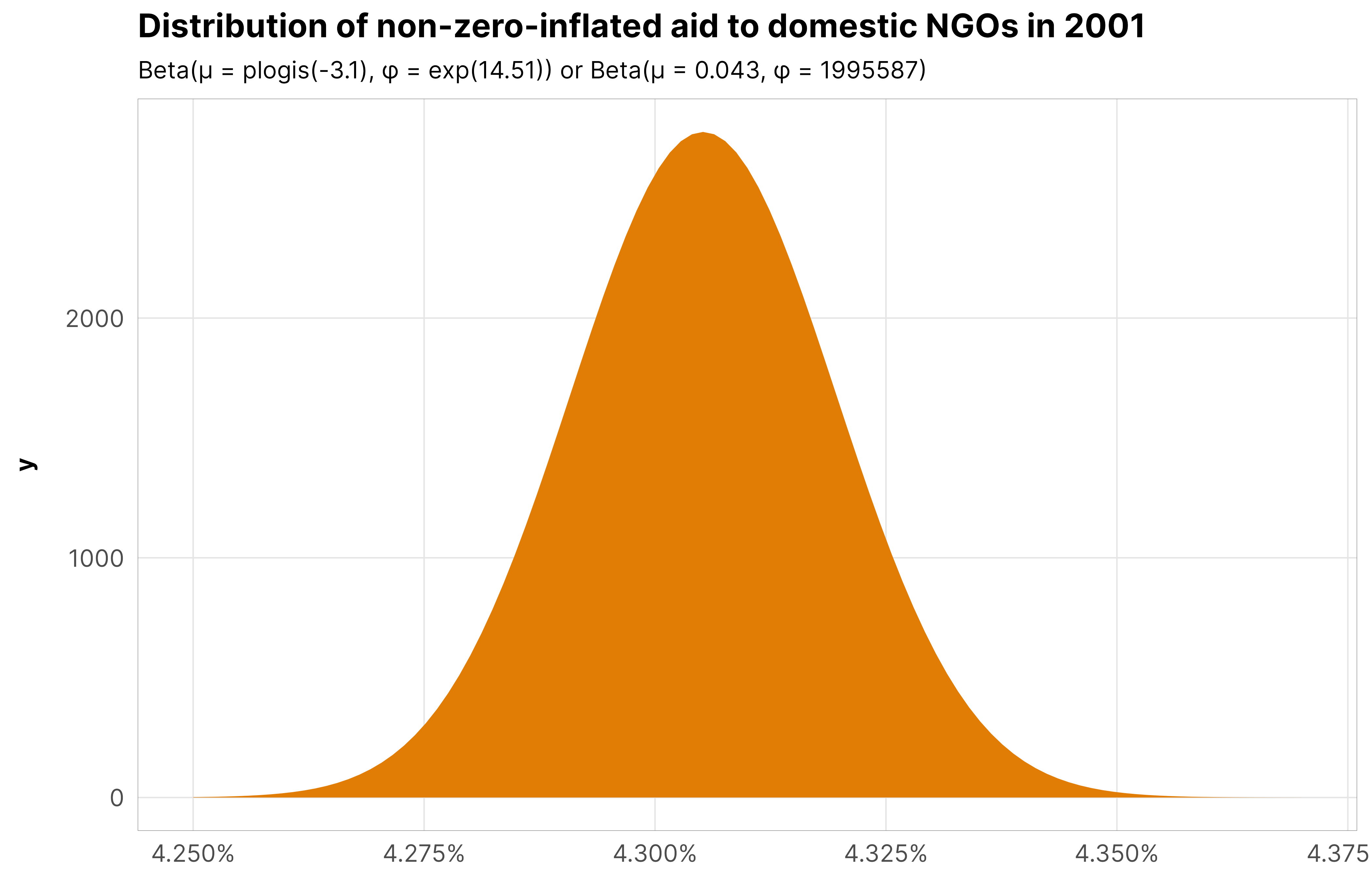
$\phi_y$ (phi): the precision or variance of aid to domestic NGOs within countries. On the log scale, it’s 14.51, which is 1,995,587 when unlogged or exponentiated, which is incredibly precise. That gives us a posterior distribution of the non-zero-inflated part of the model of $\operatorname{Beta}(0.043, 1.996\times 10^{6})$ which looks like this, very narrowly focused around the baseline average 2001 proportion:

Code

beta_params <- m_recip_outcome_total_dom$model %>% 
  tidy(parameters = c("b_(Intercept)", "phi"))

beta_mu <- beta_params %>% 
  filter(term == "b_(Intercept)") %>% 
  pull(estimate)

beta_phi <- beta_params %>% 
  filter(term == "phi") %>% 
  pull(estimate)

ggplot() +
  stat_function(geom = "area", fill = clrs$Prism[7],
                fun = ~dprop(., mean = plogis(beta_mu), size = exp(beta_phi))) +
  scale_x_continuous(labels = label_percent(), limits = c(0.0425, 0.0437)) +
  labs(title = "Distribution of non-zero-inflated aid to domestic NGOs in 2001",
       subtitle = glue::glue("Beta(µ = plogis({round(beta_mu, 2)}), φ = exp({round(beta_phi, 2)})) or Beta(µ = {round(plogis(beta_mu), 3)}, φ = {round(exp(beta_phi), 0)})")) +
  theme_donors()

$\sigma_0$ (sd__(Intercept) for the gwcode group): the variability between countries’ baseline averages, or the variability around the $b_{0_j}$ offsets. Here it’s 1.48, which means that across or between countries, the proportion of aid to domestic NGOs varies by 1.5ish logit units.
$\sigma_3$ (sd__year_c for the gwcode group): the variability between countries’ year effects, or the variability around the $b_{3_j}$ offsets. Here it’s 0.16, which means that average year effects vary by 0.15ish logit units across or between countries.

Code

m_recip_outcome_total_dom$model %>% 
  tidy(parameters = c("sd_*", "phi")) %>% 
  select(-component)
## # A tibble: 3 × 5
##   term                   estimate std.error conf.low conf.high
##   <chr>                     <dbl>     <dbl>    <dbl>     <dbl>
## 1 sd_gwcode__(Intercept)    1.48     0.131     1.25      1.76 
## 2 sd_gwcode__year_c         0.155    0.0182    0.122     0.193
## 3 phi                      14.5      0.804    13.0      16.1

Full results table

Again, this is less important since we don’t care about individual coefficients and instead care about conditional effects, but for the sake of full transparency (and to placate future reviewers), here’s a table of all the results:

% of aid to domestic NGO recipients
% of aid to foreign NGO recipients

Code

models_tbl_h3_outcome_dejure_dom <- models_tbl_h3_outcome_dejure_dom %>% 
  set_names(1:length(.))

notes <- c(
  "Posterior medians; 95% credible intervals (HDPI) in brackets.", 
  "Total \\(R^2\\) considers the variance of both population and group effects;", 
  "marginal \\(R^2\\) only takes population effects into account"
)

modelsummary(models_tbl_h3_outcome_dejure_dom,
             estimate = "{estimate}",
             statistic = "[{conf.low}, {conf.high}]",
             add_rows = outcome_rows,
             coef_map = coefs_outcome,
             gof_map = gofs,
             output = "kableExtra",
             fmt =  list(estimate = 2, conf.low = 2, conf.high = 2)) %>% 
  row_spec(1, bold = TRUE) %>% 
  kable_styling(htmltable_class = "table-sm light-border") %>% 
  footnote(general = notes, footnote_as_chunk = TRUE)

Table 2: Results from all outcome models
	1	2	3	4
Treatment	Total barriers (t)	Barriers to advocacy (t)	Barriers to entry (t)	Barriers to funding (t)
Treatment (t − 1)	0.08	−0.26	0.16	0.19
	[−0.004, 0.17]	[−0.62, 0.10]	[−0.0005, 0.32]	[0.01, 0.37]
Treatment history	−0.004	0.01	−0.01	−0.008
	[−0.01, 0.004]	[−0.02, 0.05]	[−0.03, 0.005]	[−0.02, 0.008]
Intercept	−3.10	−2.87	−2.98	−3.09
	[−3.42, −2.78]	[−3.28, −2.46]	[−3.31, −2.65]	[−3.40, −2.79]
Year	0.03	0.02	0.04	0.03
	[−0.0004, 0.07]	[−0.02, 0.06]	[−0.0008, 0.07]	[0.001, 0.07]
Zero-inflated part: Year	−0.24	−0.24	−0.18	−0.27
	[−0.38, −0.10]	[−0.38, −0.11]	[−0.32, −0.05]	[−0.41, −0.14]
Zero-inflated part: Year²	0.01	0.01	0.008	0.01
	[0.0005, 0.02]	[0.004, 0.02]	[−0.003, 0.02]	[0.004, 0.02]
Zero-inflated part: Intercept	−0.16	−0.31	−0.24	−0.11
	[−0.53, 0.20]	[−0.67, 0.05]	[−0.61, 0.13]	[−0.47, 0.25]
Between-country intercept variability ($\sigma_0$ for $b_0$ offsets)	1.48	2.13	1.55	1.45
	[1.25, 1.76]	[1.79, 2.55]	[1.29, 1.87]	[1.22, 1.72]
Between-country year variability ($\sigma_3$ for $b_3$ offsets)	0.15	0.22	0.16	0.15
	[0.12, 0.19]	[0.18, 0.26]	[0.13, 0.20]	[0.12, 0.18]
Correlation between random intercepts and slopes ($\rho$)	−0.75	−0.84	−0.76	−0.74
	[−0.84, −0.62]	[−0.90, −0.77]	[−0.84, −0.63]	[−0.83, −0.61]
Model dispersion ($\phi_y$)	14.49	14.88	12.57	14.49
	[12.97, 16.14]	[13.30, 16.55]	[11.15, 14.12]	[13.04, 16.08]
N	1676	1676	1676	1676
$R^2$ (total)	0.43	0.46	0.44	0.42
$R^2$ (marginal)	0.008	0.004	0.008	0.009
Note: Posterior medians; 95% credible intervals (HDPI) in brackets. Total $R^2$ considers the variance of both population and group effects; marginal $R^2$ only takes population effects into account

Code

models_tbl_h3_outcome_dejure_foreign <- models_tbl_h3_outcome_dejure_foreign %>% 
  set_names(1:length(.))

notes <- c(
  "Posterior medians; 95% credible intervals (HDPI) in brackets.", 
  "Total \\(R^2\\) considers the variance of both population and group effects;", 
  "marginal \\(R^2\\) only takes population effects into account"
)

modelsummary(models_tbl_h3_outcome_dejure_foreign,
             estimate = "{estimate}",
             statistic = "[{conf.low}, {conf.high}]",
             add_rows = outcome_rows,
             coef_map = coefs_outcome,
             gof_map = gofs,
             output = "kableExtra",
             fmt =  list(estimate = 2, conf.low = 2, conf.high = 2)) %>% 
  row_spec(1, bold = TRUE) %>% 
  kable_styling(htmltable_class = "table-sm light-border") %>% 
  footnote(general = notes, footnote_as_chunk = TRUE)

Table 3: Results from all outcome models
	1	2	3	4
Treatment	Total barriers (t)	Barriers to advocacy (t)	Barriers to entry (t)	Barriers to funding (t)
Treatment (t − 1)	0.02	0.18	0.06	0.03
	[−0.05, 0.09]	[−0.12, 0.47]	[−0.07, 0.18]	[−0.12, 0.18]
Treatment history	0.002	−0.002	−0.002	0.007
	[−0.004, 0.009]	[−0.02, 0.02]	[−0.01, 0.01]	[−0.007, 0.02]
Intercept	−0.80	−0.78	−0.77	−0.77
	[−1.04, −0.56]	[−1.03, −0.53]	[−1.02, −0.54]	[−1.00, −0.54]
Year	−0.05	−0.05	−0.04	−0.05
	[−0.08, −0.02]	[−0.07, −0.02]	[−0.07, −0.02]	[−0.07, −0.02]
Zero-inflated part: Year	−0.04	−0.06	0.02	−0.09
	[−0.19, 0.11]	[−0.21, 0.09]	[−0.13, 0.17]	[−0.23, 0.06]
Zero-inflated part: Year²	0.0004	0.006	−0.002	0.004
	[−0.01, 0.01]	[−0.006, 0.02]	[−0.01, 0.009]	[−0.007, 0.02]
Zero-inflated part: Intercept	−1.13	−1.31	−1.18	−1.05
	[−1.55, −0.73]	[−1.74, −0.90]	[−1.60, −0.78]	[−1.46, −0.65]
Between-country intercept variability ($\sigma_0$ for $b_0$ offsets)	1.19	1.26	1.16	1.21
	[1.01, 1.40]	[1.07, 1.48]	[0.99, 1.37]	[1.03, 1.42]
Between-country year variability ($\sigma_3$ for $b_3$ offsets)	0.11	0.12	0.10	0.11
	[0.09, 0.14]	[0.09, 0.14]	[0.08, 0.13]	[0.09, 0.14]
Correlation between random intercepts and slopes ($\rho$)	−0.70	−0.73	−0.68	−0.71
	[−0.80, −0.55]	[−0.82, −0.58]	[−0.79, −0.52]	[−0.81, −0.57]
Model dispersion ($\phi_y$)	8.64	8.65	8.00	8.72
	[7.93, 9.39]	[7.96, 9.39]	[7.29, 8.74]	[8.01, 9.47]
N	1676	1676	1676	1676
$R^2$ (total)	0.34	0.36	0.33	0.35
$R^2$ (marginal)	0.01	0.02	0.01	0.02
Note: Posterior medians; 95% credible intervals (HDPI) in brackets. Total $R^2$ considers the variance of both population and group effects; marginal $R^2$ only takes population effects into account

References

Keele, Luke, Randolph T. Stevenson, and Felix Elwert. 2020. “The Causal Interpretation of Estimated Associations in Regression Models.” Political Science Research and Methods 8 (1): 1–13. https://doi.org/10.1017/psrm.2019.31.

Westreich, Daniel, and Sander Greenland. 2013. “The Table 2 Fallacy: Presenting and Interpreting Confounder and Modifier Coefficients.” American Journal of Epidemiology 177 (4): 292–98. https://doi.org/10.1093/aje/kws412.