library(tidyverse)library(targets)library(brms)library(tidybayes)library(broom)library(broom.mixed)library(modelsummary)library(marginaleffects)library(patchwork)library(scales)library(ggdist)library(ggtext)library(ggh4x)library(kableExtra)library(glue)library(here)tar_config_set(store = here::here('_targets'),script = here::here('_targets.R'))set.seed(1234)# Load stuff from targets# Plotting functionsinvisible(list2env(tar_read(graphic_functions), .GlobalEnv))invisible(list2env(tar_read(tbl_functions), .GlobalEnv))set_annotation_fonts()# Tell bayesplot to use the sunset palette for things like pp_check()bayesplot::color_scheme_set(clrs$Sunset[2:7])# Datadf_country_aid <-tar_read(country_aid_final)df_country_aid_laws <-filter(df_country_aid, laws)# Treatment modelstar_load(c(m_oda_treatment_total, m_oda_treatment_advocacy, m_oda_treatment_entry, m_oda_treatment_funding, m_oda_treatment_ccsi, m_oda_treatment_repress))# IPTW datatar_load(c(df_oda_iptw_total, df_oda_iptw_advocacy, df_oda_iptw_entry, df_oda_iptw_funding, df_oda_iptw_ccsi, df_oda_iptw_repress))# Outcome modelstar_load(c(m_oda_outcome_total, m_oda_outcome_advocacy, m_oda_outcome_entry, m_oda_outcome_funding, m_oda_outcome_ccsi, m_oda_outcome_repress))# Marginal/conditional effectstar_load(c(mfx_oda_cfx_multiple, mfx_oda_cfx_single))# Results tablestar_load(c(models_tbl_h1_treatment_num, models_tbl_h1_treatment_denom))tar_load(c(models_tbl_h1_outcome_dejure, models_tbl_h1_outcome_defacto))
Code
invisible(list2env(tar_read(modelsummary_functions), .GlobalEnv))treatment_names <-c("Treatment", "Total barriers (t)", "Barriers to advocacy (t)", "Barriers to entry (t)", "Barriers to funding (t)", "CCSI (t)","CS repression (t)")treatment_rows <-as.data.frame(t(treatment_names))attr(treatment_rows, "position") <-1outcome_names <-c("Treatment", "Total barriers (t)", "Barriers to advocacy (t)", "Barriers to entry (t)", "Barriers to funding (t)")outcome_rows <-as.data.frame(t(outcome_names))attr(outcome_rows, "position") <-1
Weight models
General idea
To create stabilized inverse probability of treatment weights (IPTW) for a continuous treatment, we calculate the ratio of two distributions:
The numerator is the probability distribution \(\phi\) of treatment \(X_{it}\), given lagged treatment \(X_{i, t-1}\), treatment history \(\sum_{\tau = (t-2)}^{t} X_{i\tau}\), and non-time-varying confounders \(Z_i\)
The denominator is the probability distribution \(\phi\) of treatment \(X_{it}\), given lagged treatment \(X_{i, t-1}\), treatment history \(\sum_{\tau = (t-2)}^{t} X_{i\tau}\), lagged outcome \(Y_{i, t-1}\), time-varying confounders \(Z_{it}\), and non-time-varying confounders \(Z_i\)
We then calculate the cumulative product of this ratio for each year within each country:
In general code, here’s what that process looks like:
Code
# We don't actually use lm() in the project; this is just a general illustration# of the idea of building the weightsmodel_num <-lm(treatment ~ treatment_lag1 + treatment_lag2_cumsum + confounders_no_time)distribution_num <-dnorm(data$treatment, mean =predict(model_num),sd =sd(residuals(model_num)))model_denom <-lm(treatment ~ treatment_lag1 + treatment_lag2_cumsum + outcome_lag1 + confounders_time_varying + counfounders_no_time)distribution_denom <-dnorm(data$treatment, mean =predict(model_denom),sd =sd(residuals(model_denom)))data <- data %>%mutate(weights_ratio = distribution_num / distribution_denom) %>%group_by(gwcode) %>%mutate(iptw =cumprod(weights_ratio)) %>%ungroup()
Actual models
We identify our time-varying and time-invariant confounders based on our causal model and do-calculus logic, and we deal with the panel structure of the data by including random intercepts for country, and both a population-level trend and random slopes for year. We use generic weakly informative priors for our model parameters.
Numerator
Our numerator models look like this (but with the actual treatment variable replacing treatment, like barriers_total, advocacy, and so on):
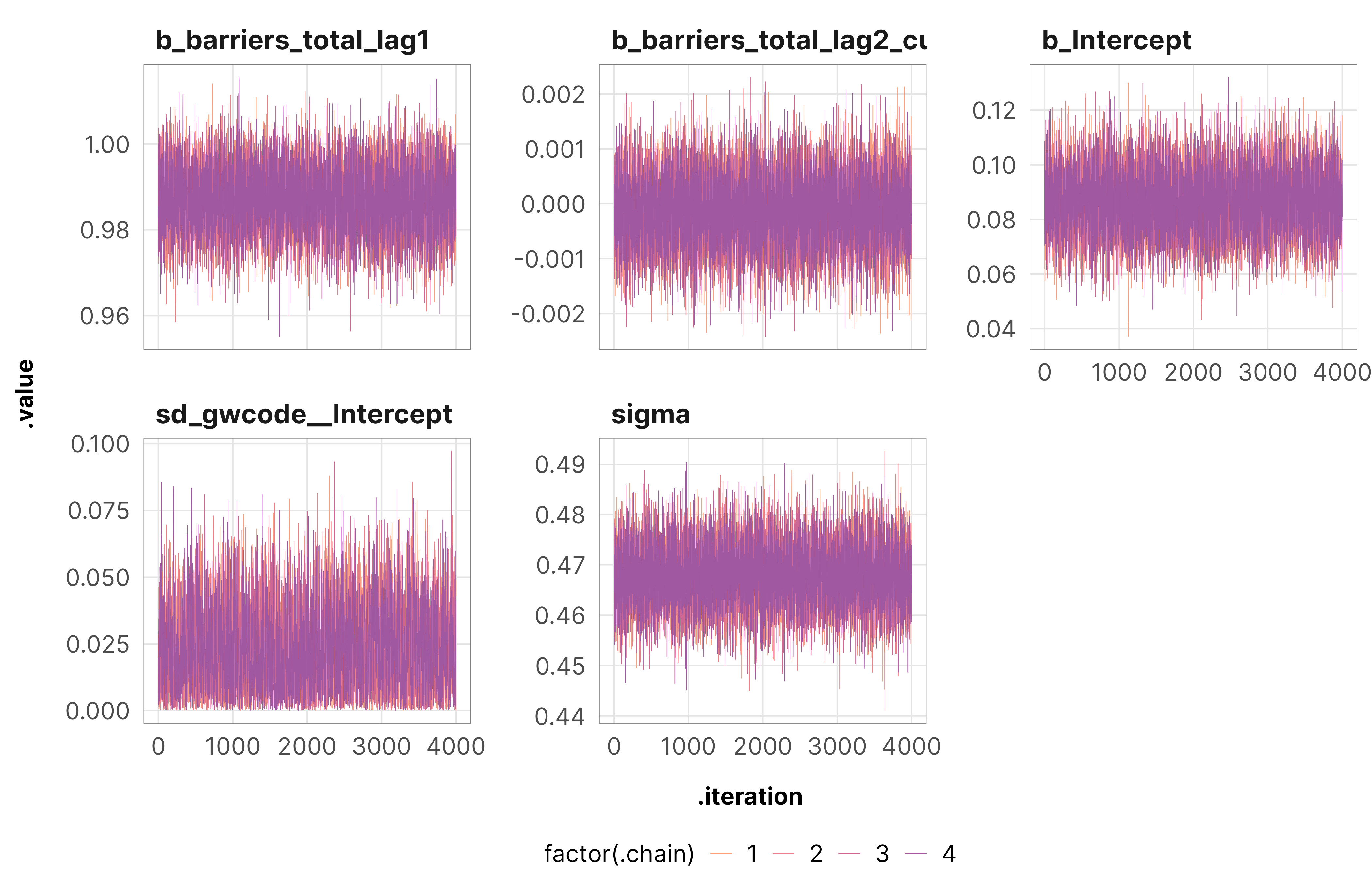
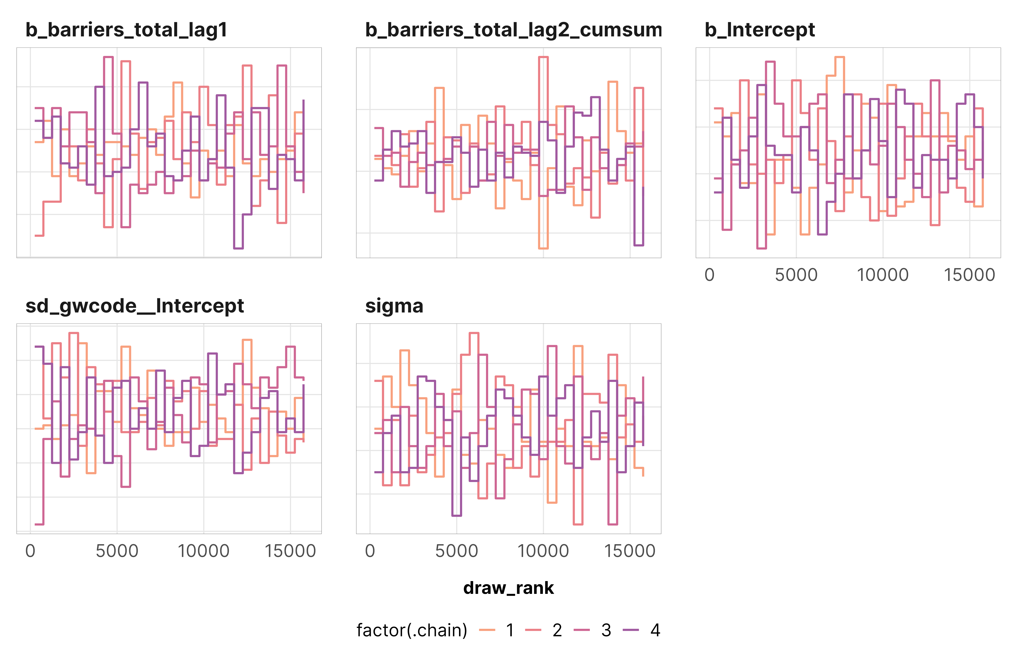
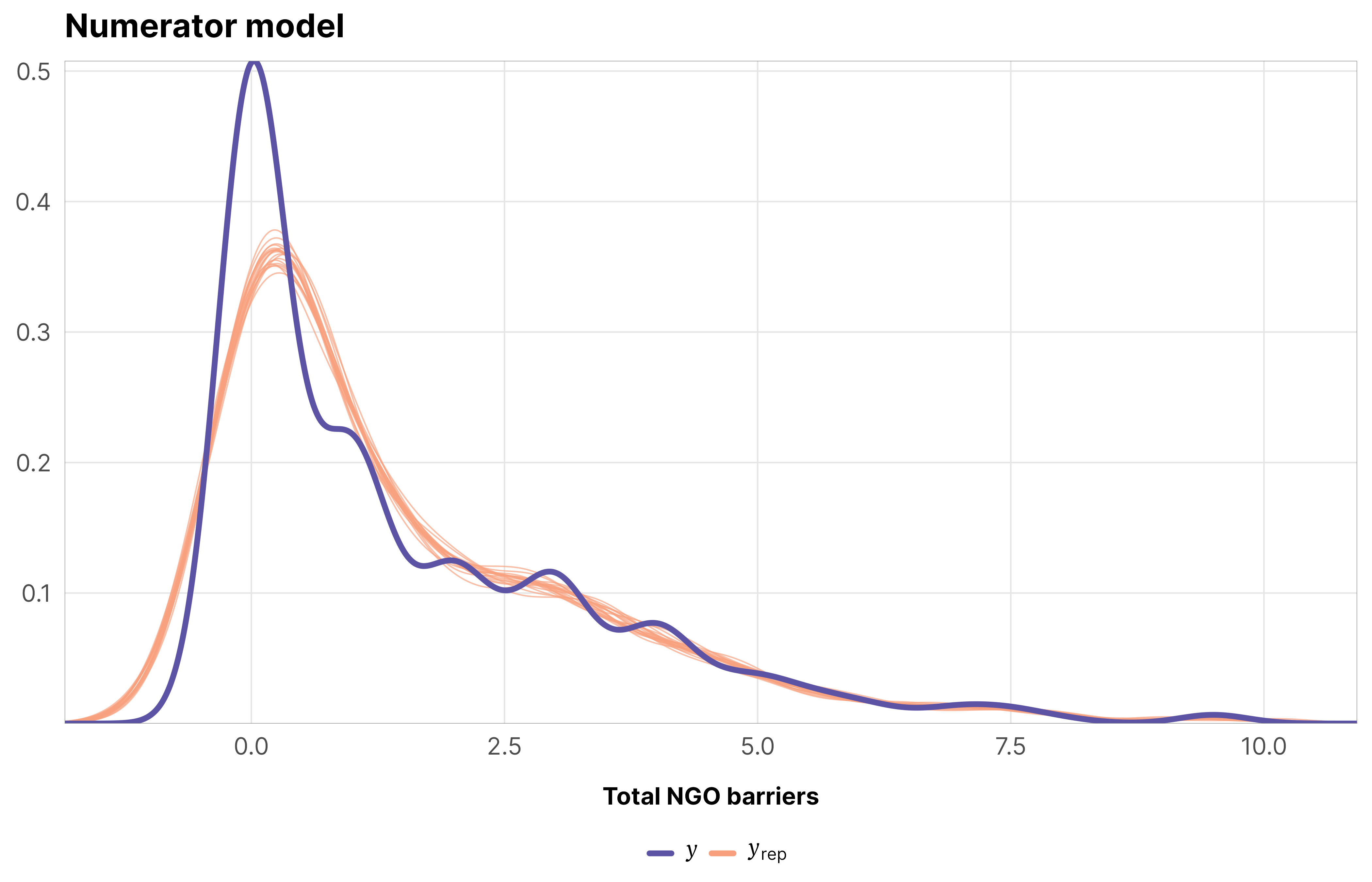
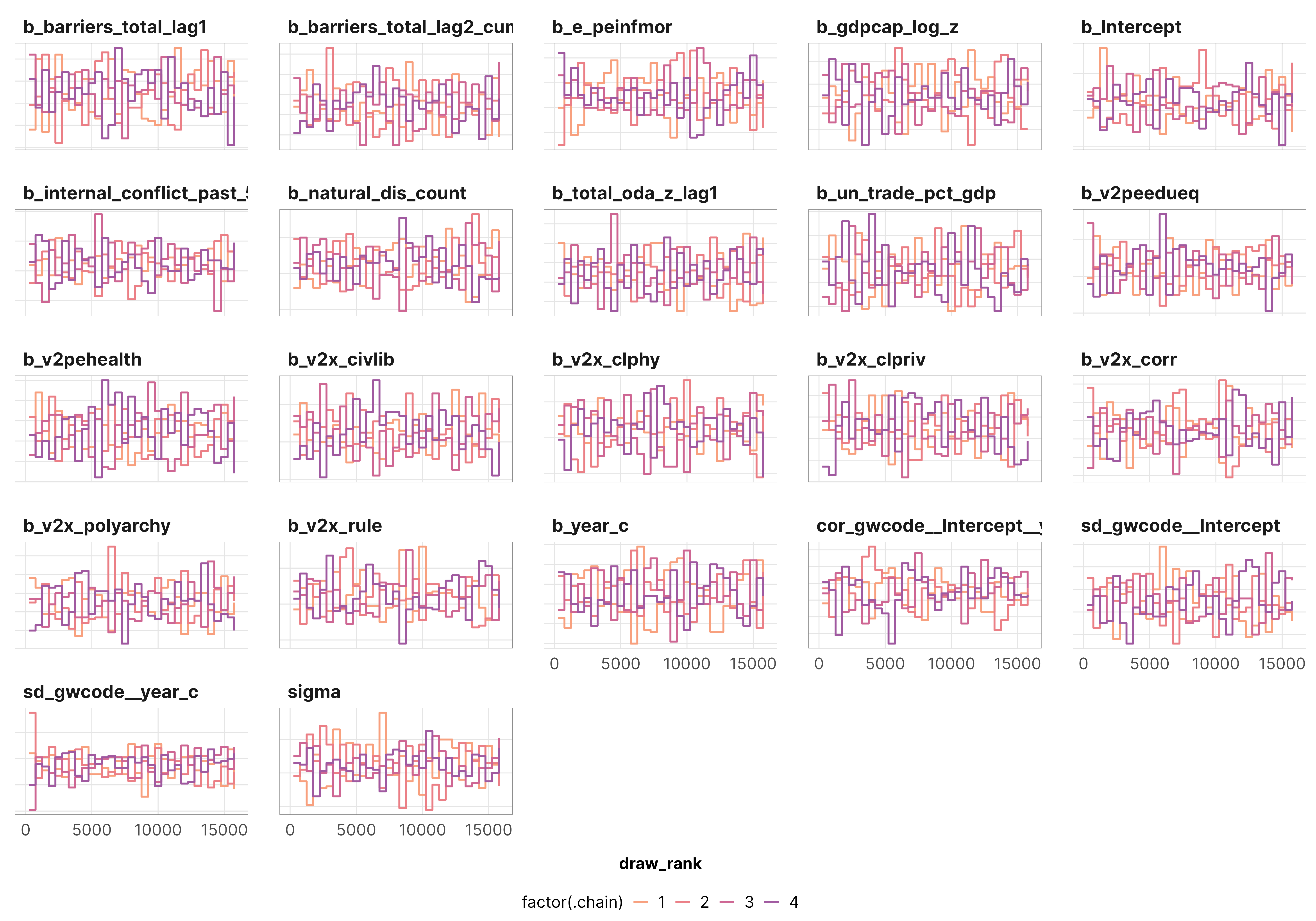
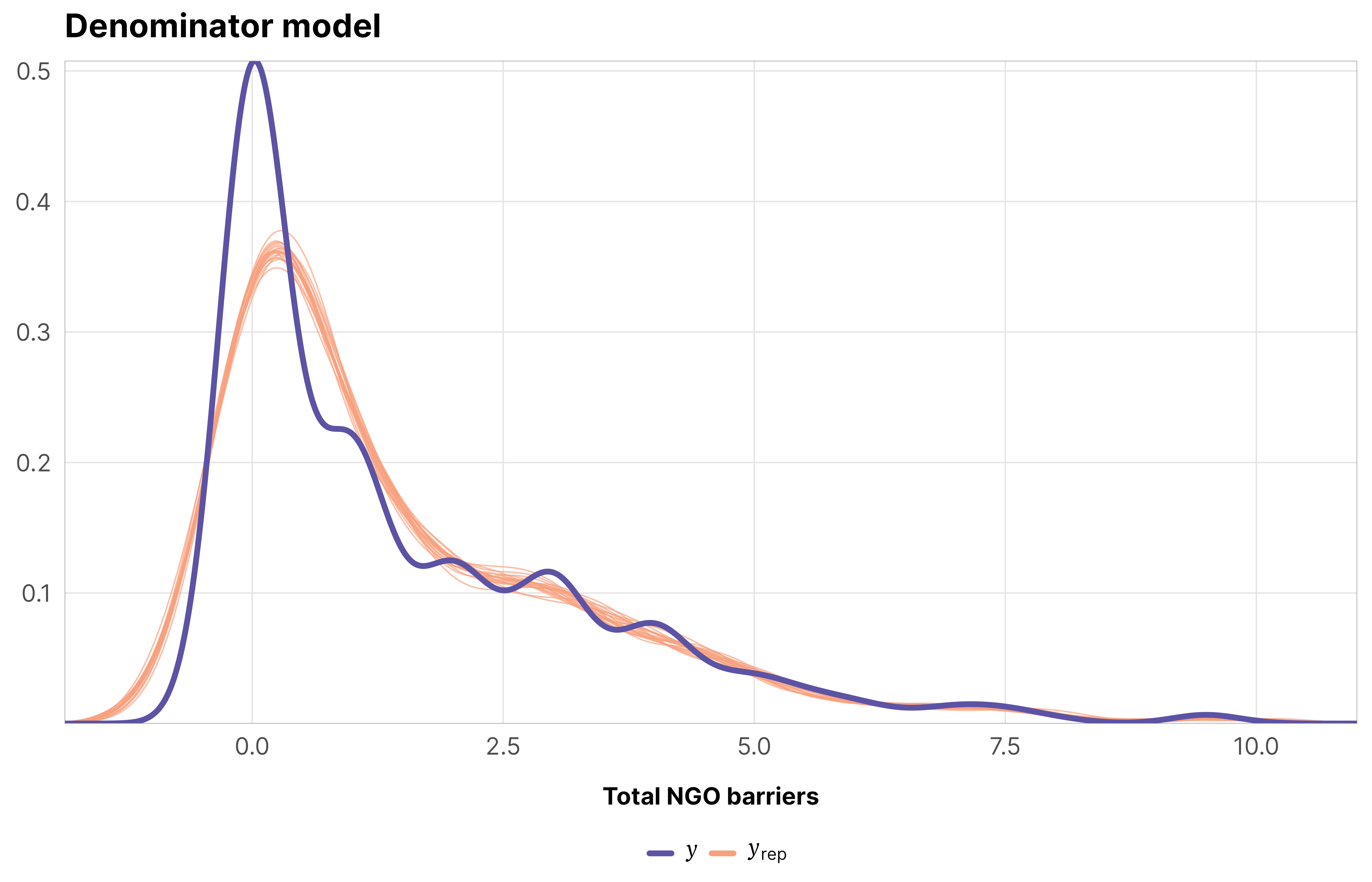
Just to make sure everything converged nicely, we check some diagnostics for the weight models for the total barriers treatment. All the other models look basically the same as this—everything’s fine.
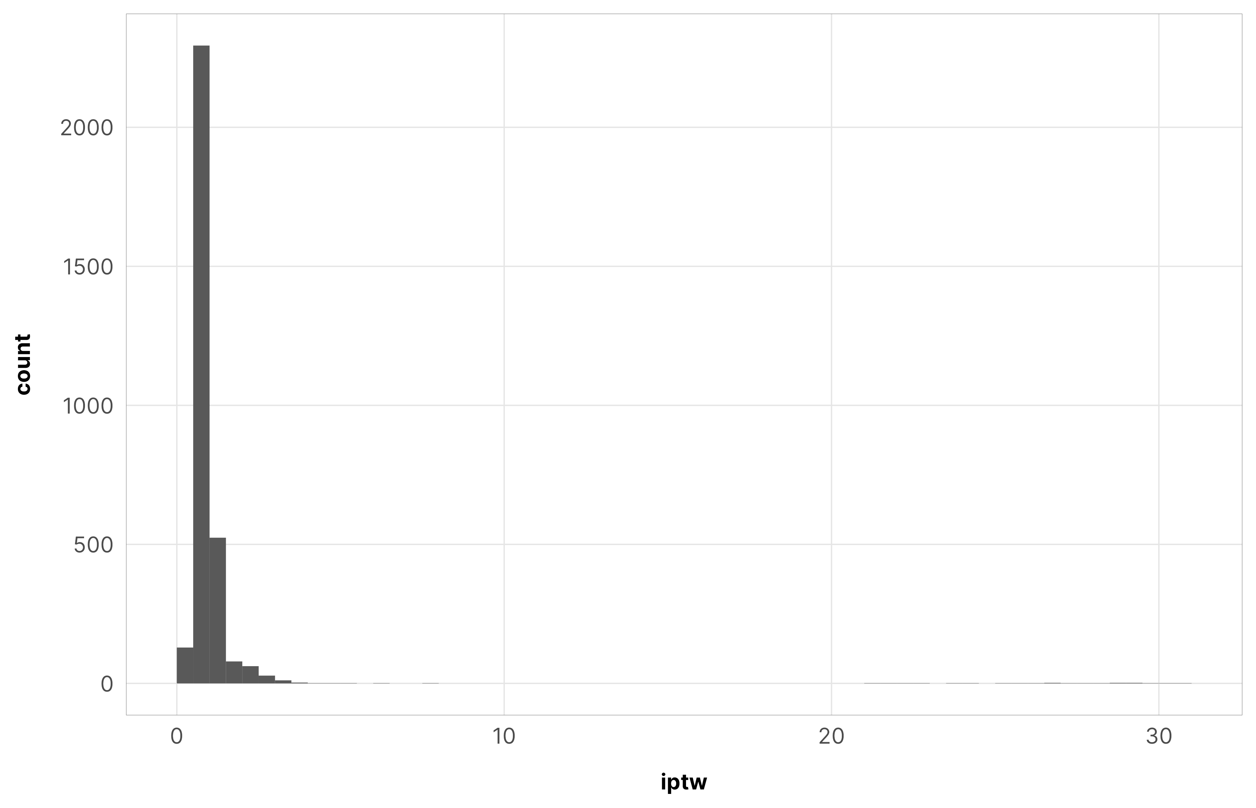
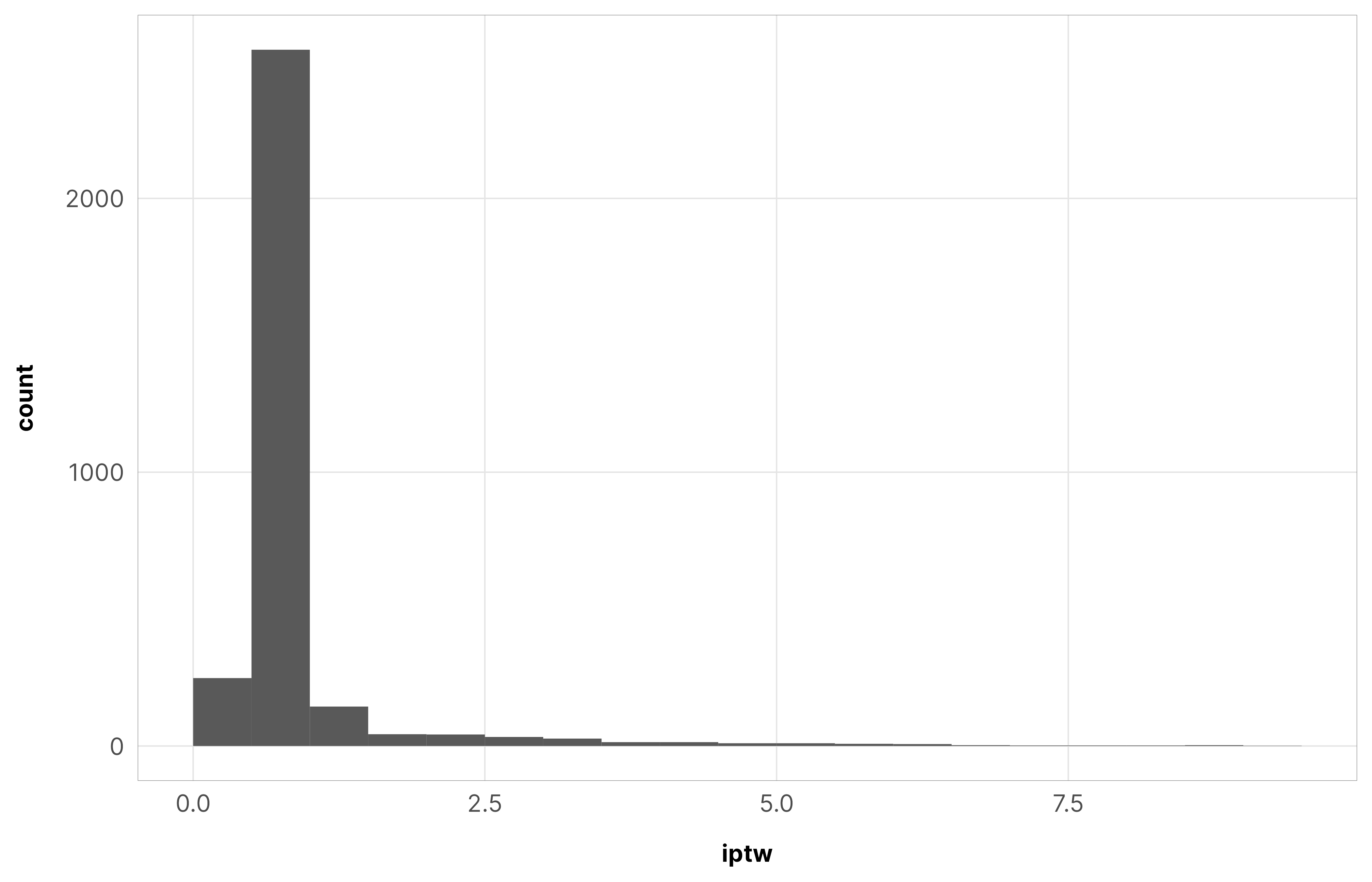
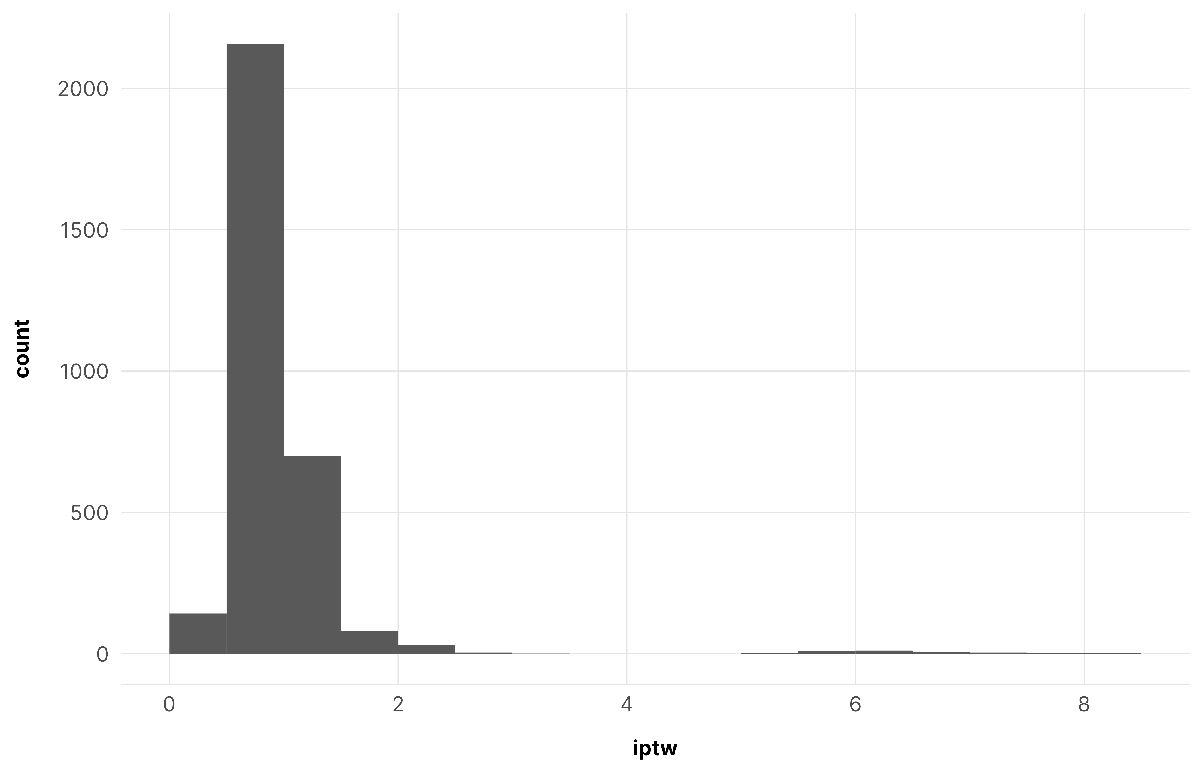
IPTWs should generally have a mean of 1 and shouldn’t be too incredibly high. When they’re big, it’s a good idea to truncate them at some reasonable level.
The max weight here is 31, but there are only a handful of observations with weights that high. The average is 1.13 and the median is 0.91, which are both close to 1, so we’re good.
Code
summary(df_oda_iptw_total$iptw)## Min. 1st Qu. Median Mean 3rd Qu. Max. ## 0.05 0.78 0.91 1.13 1.00 30.65
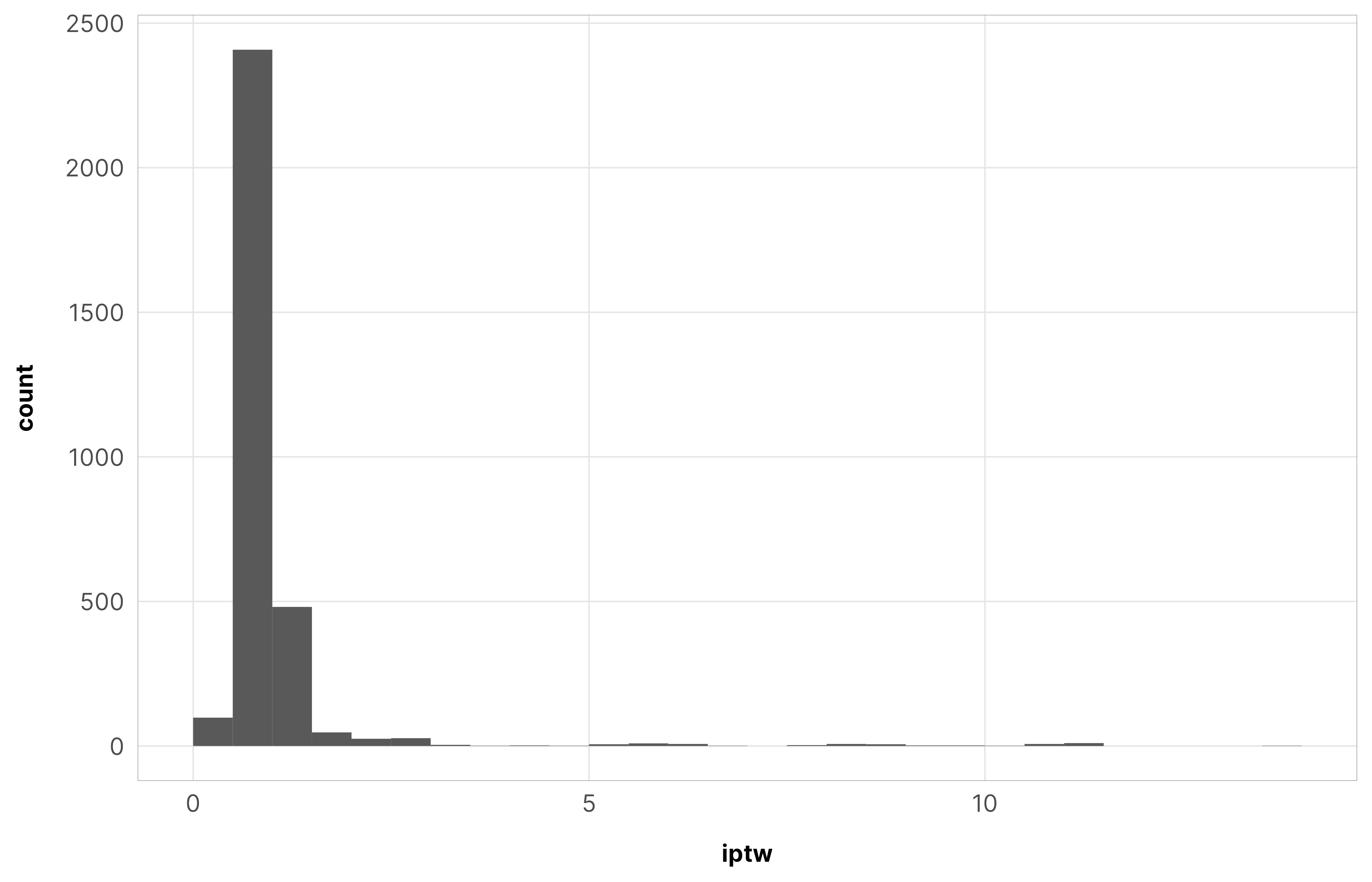
lol these blow up. The max weight is 9,851,384,166,626, which, oh no.
Code
summary(df_oda_iptw_ccsi$iptw)## Min. 1st Qu. Median Mean 3rd Qu. Max. ## 0.00e+00 0.00e+00 0.00e+00 2.16e+10 0.00e+00 9.85e+12
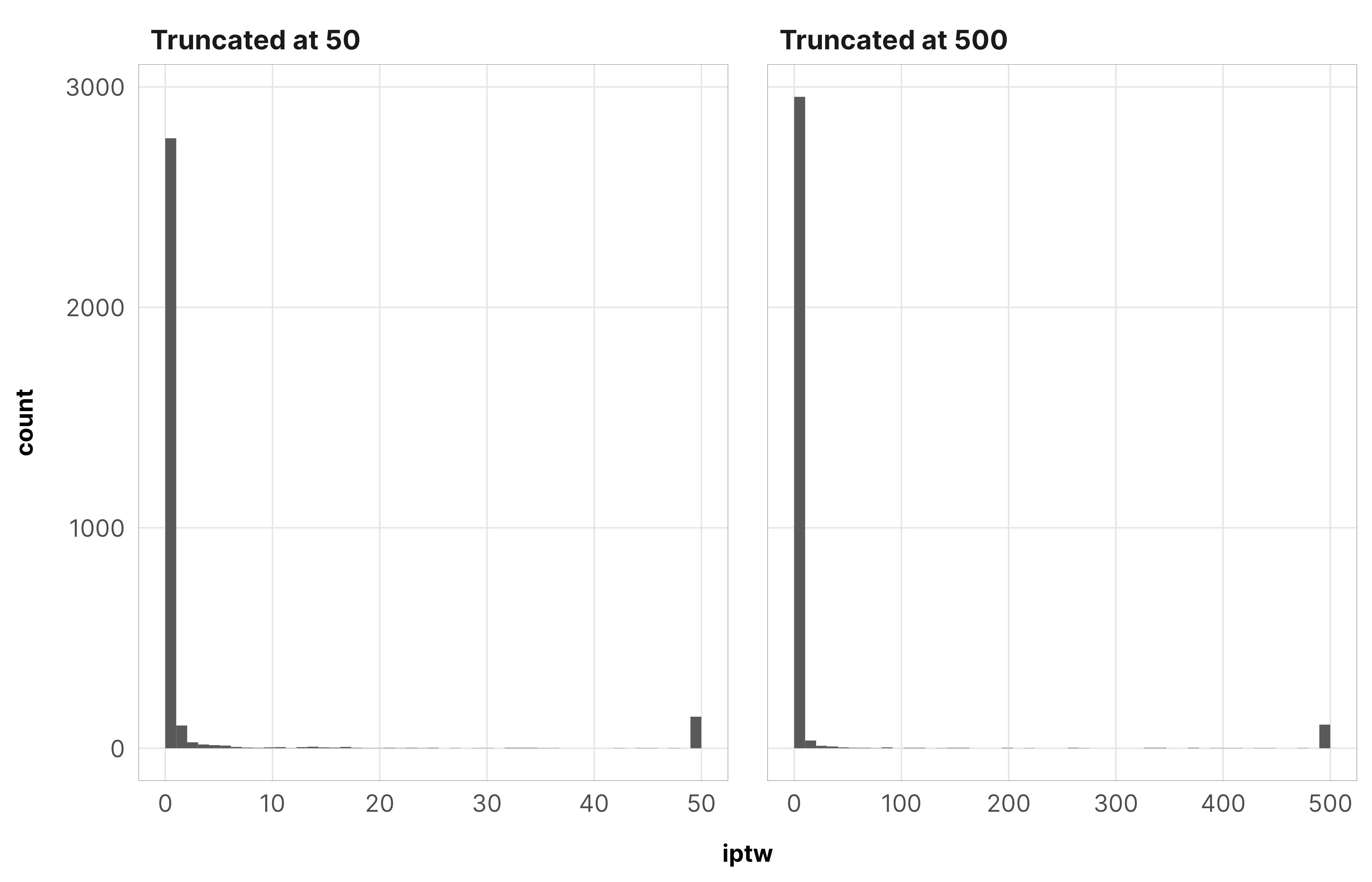
There aren’t a lot of observations with weights that high though. Check out the counts of rows with weights greater than 50 and greater than 500—only 100ish:
We truncate these weights at 50. For robustness checks, we also truncate at 500, but (1) those models take substantially longer to run, and (2) the results are roughly the same.
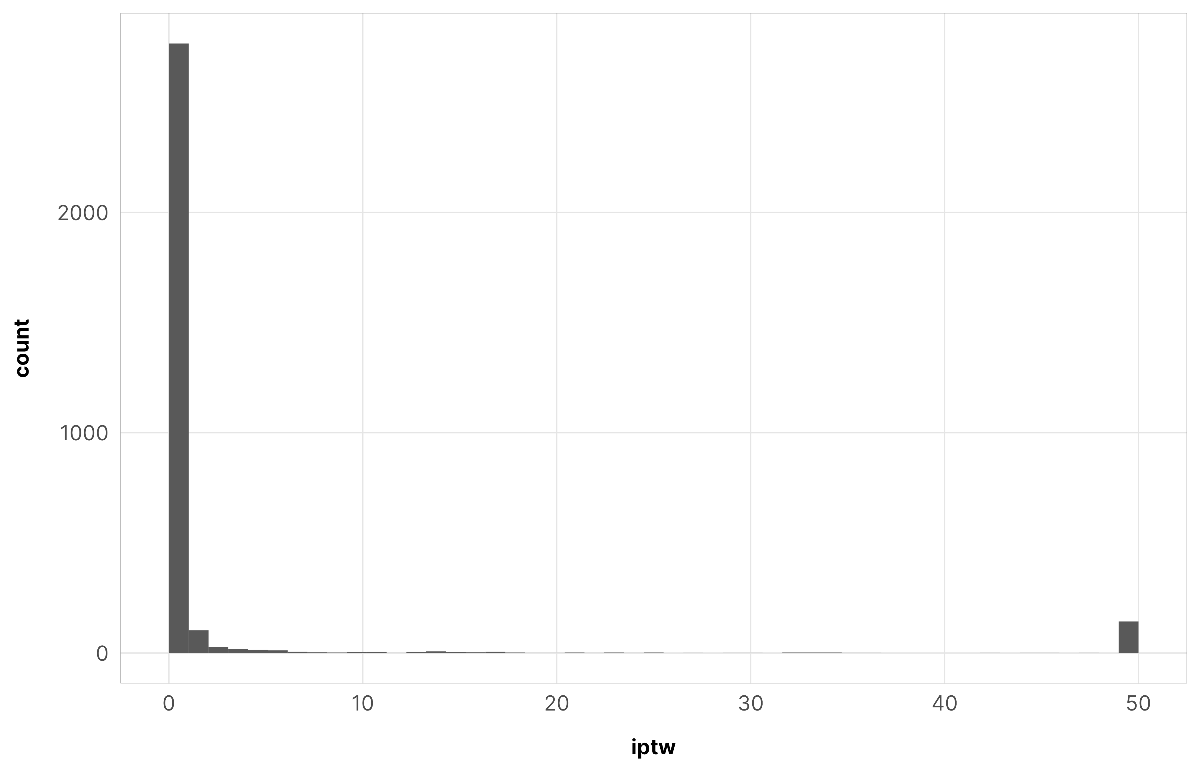
So we truncate these weights at 50 again. Since the results from the core civil society models are basically the same when truncating at 500, we only use a truncation point of 50 here.
These are less important since we just use these treatment models to generate weights and because interpreting each coefficient when trying to isolate causal effects is unimportant (Westreich and Greenland 2013; Keele, Stevenson, and Elwert 2020).
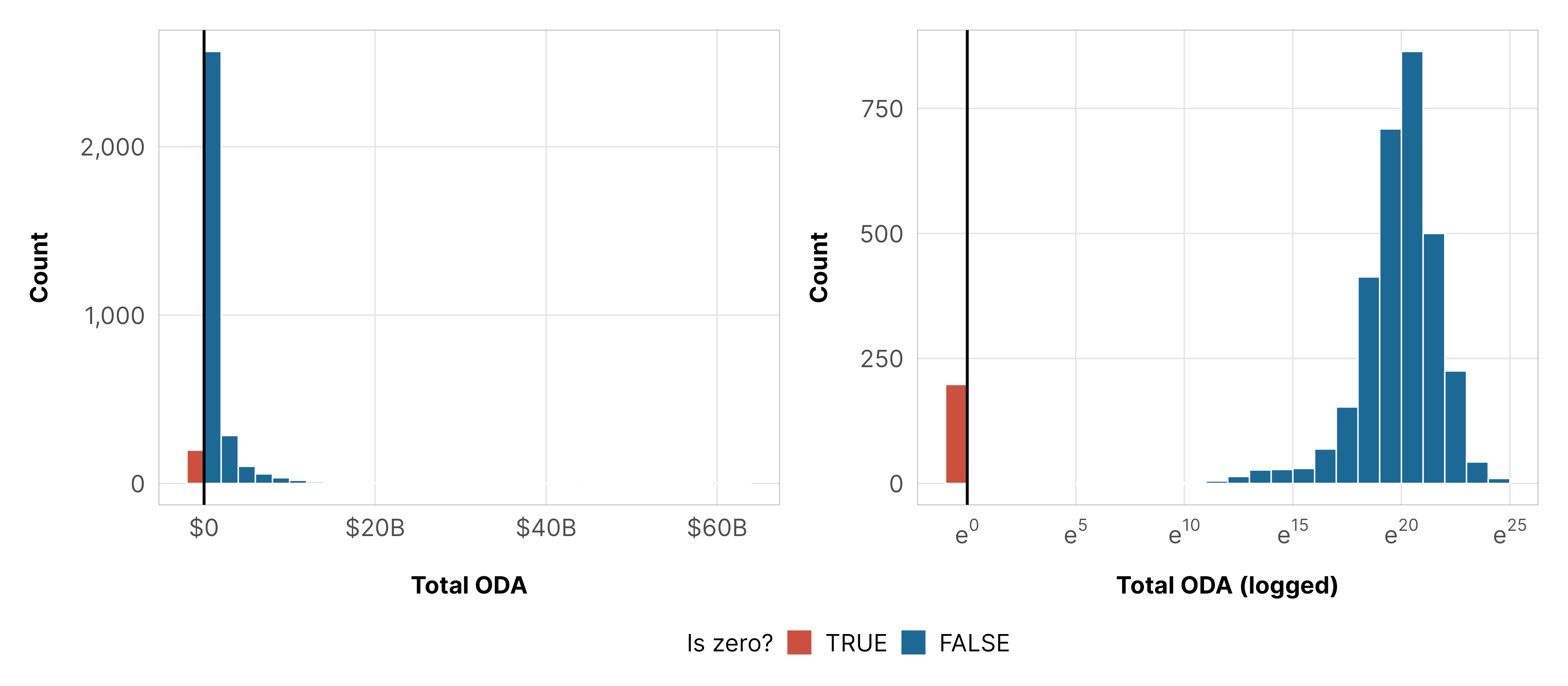
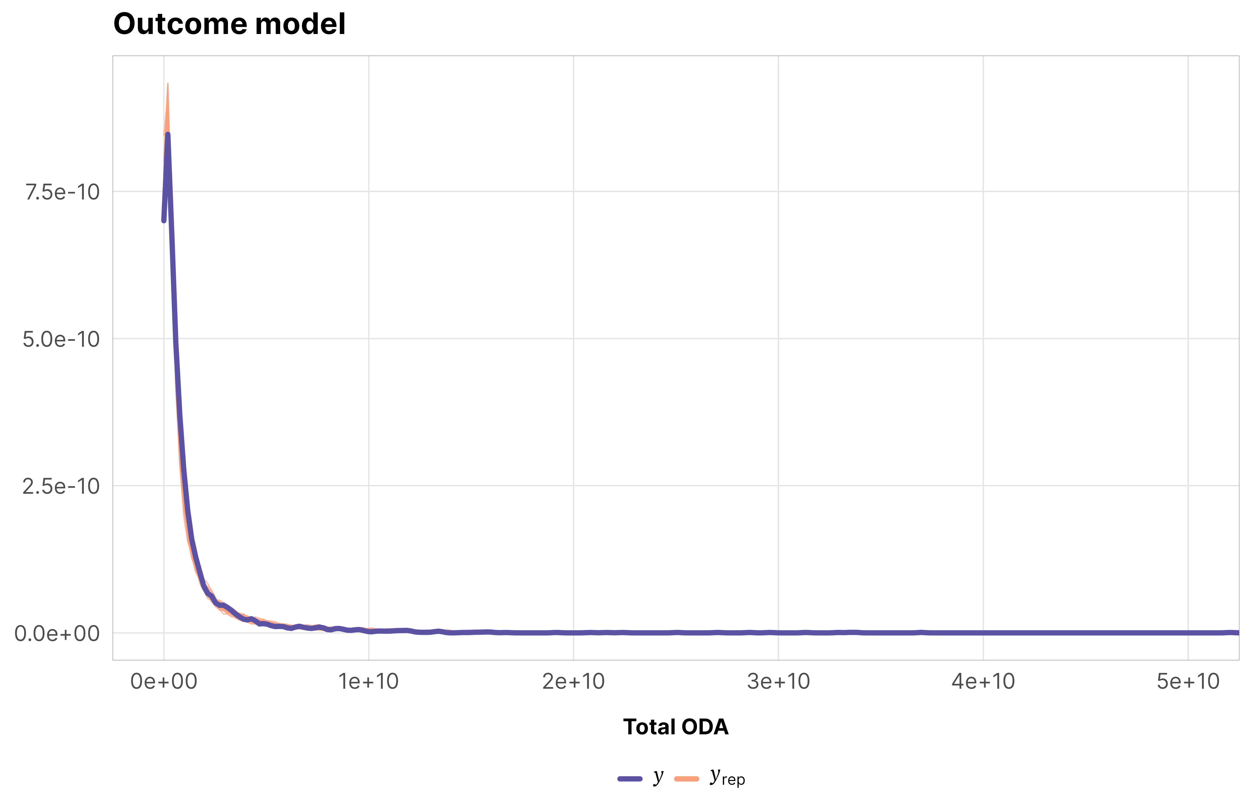
Because of this distribution, we use a hurdled lognormal family to model the outcome. This guide to working with tricky outcomes with lots of zeros explores all the intricacies of hurdled lognormal models, so we won’t go into tons of detail here.
Following our marginal structural model approach, we need to run a model weighted by the stabilized inverse probability weights that includes covariates for lagged treatment \(X_{i, t-1}\), treatment history \(\sum_{\tau = (t-2)}^{t} X_{i\tau}\), and non-time-varying confounders \(Z_i\). We expand on this approach to account for the panel structure of the data by using a multilevel hierarchical model with country-specific intercepts and a year trend with country-specific offsets (following yet another guide I wrote for this project, this one on multilevel panel data). We center the year at 2000 so that (1) the intercept is interpretable (Schielzeth 2010) and (2) the MCMC simulation runs faster and more efficiently (McElreath 2020, sec. 13.4, pp. 420–422).
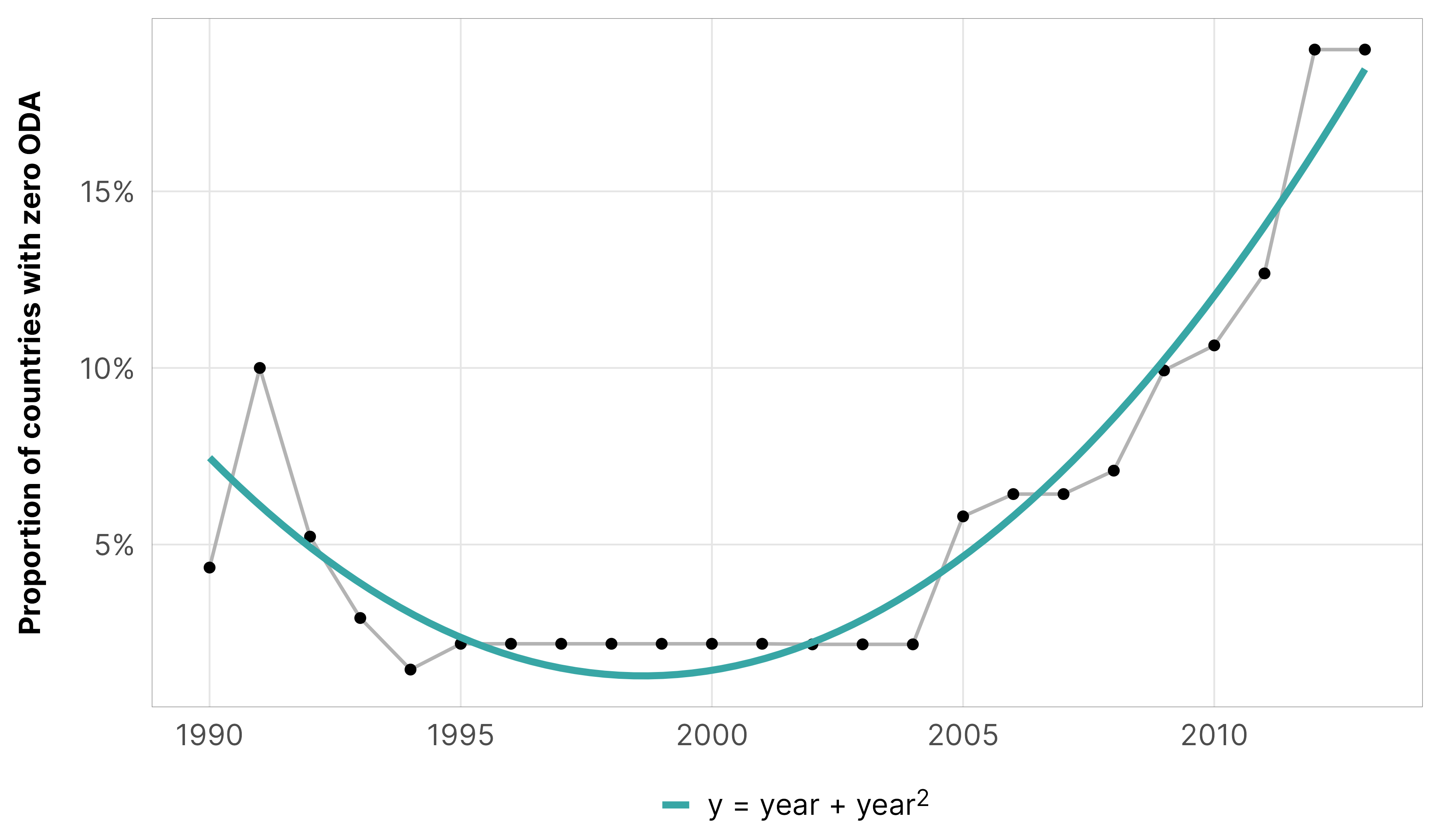
We’re not entirely sure what the actual underlying zero process is for foreign aid, but from looking at the data, we know that there’s a time component—before 1995 and after 2005 lots of countries received no aid. We don’t know why, though. Maybe there are issues with reporting quality. Maybe some countries didn’t need aid anymore (almost like a survival model, but not really, since countries can resume getting aid later after seeing a 0). Maybe there were political reasons. It’s impossible to tell, and it goes beyond the scope of our paper here. Accordingly, we model the hurdle part of the model with year and year squared since the year trend is parabolic and nonlinear.
Code
df_country_aid_laws %>%group_by(year) %>%summarize(prop_zero =mean(total_oda ==0)) %>%ggplot(aes(x = year, y = prop_zero)) +geom_line(linewidth =0.5, color ="grey70") +geom_point(size =1) +geom_smooth(aes(color ="y = year + year<sup>2</sup>"), method ="lm", formula = y ~ x +I(x^2), se =FALSE) +scale_y_continuous(labels =label_percent()) +scale_color_manual(values = clrs$Prism[c(3, 11)]) +labs(x =NULL, y ="Proportion of countries with zero ODA",color =NULL) +theme_donors() +theme(legend.text =element_markdown())
Formal model and priors
Our final model looks like this (again with treatment replaced by the actual treatment column):
\[
\begin{aligned}
&\ \mathrlap{\textbf{Hurdled model of aid $i$ across time $t$ within each country $j$}} \\
\text{Foreign aid}_{it_j} \sim&\ \mathrlap{\begin{cases}
0 & \text{with probability } \pi_{it} \\[4pt]
\operatorname{Log-normal}(\mu_{it_j}, \sigma_y) & \text{with probability } 1 - \pi_{it}
\end{cases}} \\
\\
&\ \textbf{Models for distribution parameters} \\
\operatorname{logit}(\pi_{it}) =&\ \gamma_0 + \gamma_1 \text{Year}_{it} + \gamma_2 \text{Year}^2_{it} & \text{Zero/not-zero process} \\[4pt]
\log (\mu_{it_j}) =&\ \text{IPTW}_{i, t-1_j} \times \Bigl[ (\beta_0 + b_{0_j}) + \beta_1\, \text{Treatment}_{i, t-1_j} + \\
&\ \beta_2\, \textstyle{\sum_{\tau = (t-2)}^{t}} \text{Treatment}_{i\tau} + (\beta_3 + b_{3_j}) \text{Year}_{it_j} \Bigr] & \text{Within-country variation} \\[4pt]
\left(
\begin{array}{c}
b_{0_j} \\
b_{3_j}
\end{array}
\right)
\sim&\ \text{MV}\,\mathcal{N}
\left[
\left(
\begin{array}{c}
0 \\
0 \\
\end{array}
\right)
, \,
\left(
\begin{array}{cc}
\sigma^2_{0} & \rho_{0, 3}\, \sigma_{0} \sigma_{3} \\
\cdots & \sigma^2_{3}
\end{array}
\right)
\right] & \text{Variability in average intercepts and slopes} \\
\\
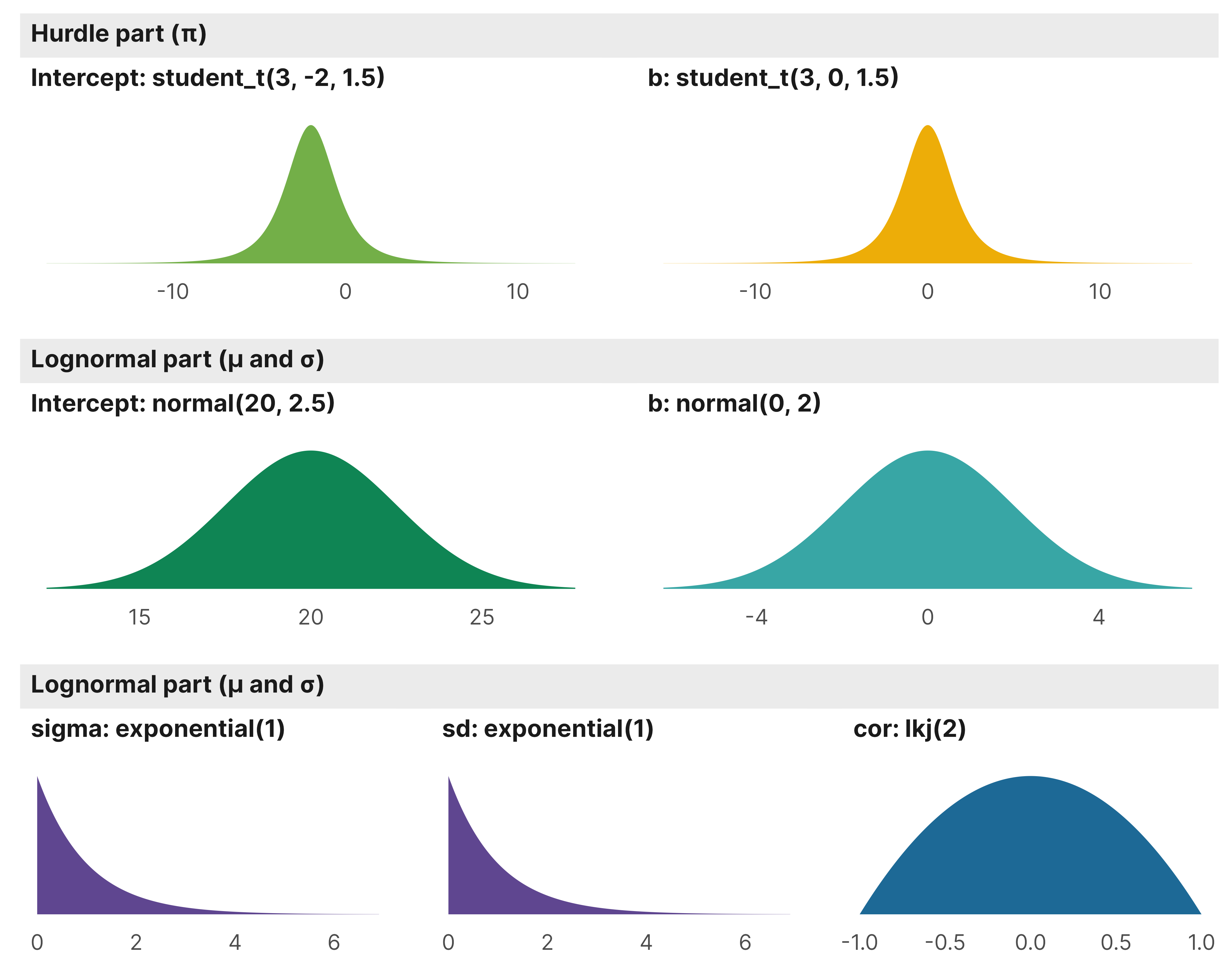
&\ \textbf{Priors} \\
\gamma_0 \sim&\ \text{Student $t$}(\nu = 3, \mu = -2, \sigma = 1.5) & \text{Prior for intercept in hurdle model} \\
\gamma_1, \gamma_2 \sim&\ \text{Student $t$}(\nu = 3, \mu = 0, \sigma = 1.5) & \text{Prior for year effect in hurdle model} \\
\beta_0 \sim&\ \mathcal{N}(20, 2.5) & \text{Prior for global average aid} \\
\beta_1, \beta_2, \beta_3 \sim&\ \mathcal{N}(0, 2) & \text{Prior for global effects} \\
\sigma_y, \sigma_0, \sigma_3 \sim&\ \operatorname{Exponential}(1) & \text{Prior for within-country variability} \\
\rho \sim&\ \operatorname{LKJ}(2) & \text{Prior for between-country variability}
\end{aligned}
\]
Here’s what those priors look like:
Code
design <-" AAABBB CCCDDD EEFFGG"m_oda_outcome_total$priors %>%parse_dist() %>%# K = dimension of correlation matrix; # ours is 2x2 here because we have one random slopemarginalize_lkjcorr(K =2) %>%mutate(nice_title =glue("**{class}**: {prior}"),stage =ifelse(dpar =="hu", "Hurdle part (π)", "Lognormal part (µ and σ)")) %>%mutate(nice_title =fct_inorder(nice_title)) %>%ggplot(aes(y =0, dist = .dist, args = .args, fill = prior)) +stat_slab(normalize ="panels") +scale_fill_manual(values = clrs$Prism[1:6]) +facet_manual(vars(stage, nice_title), design = design, scales ="free_x",strip =strip_nested(background_x =list(element_rect(fill ="grey92"), NULL),by_layer_x =TRUE)) +guides(fill ="none") +labs(x =NULL, y =NULL) +theme_donors(prior =TRUE) +theme(strip.text =element_markdown())
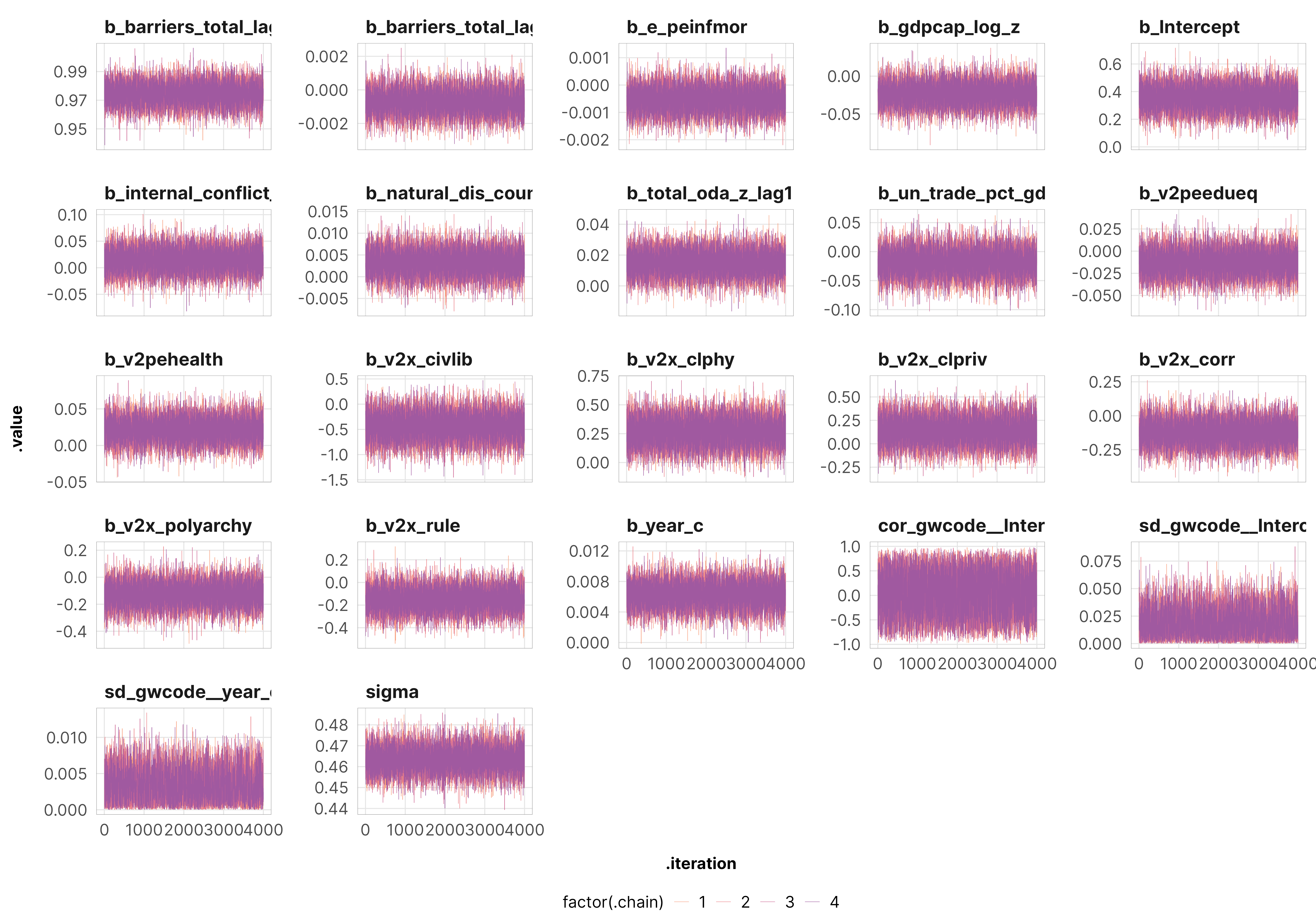
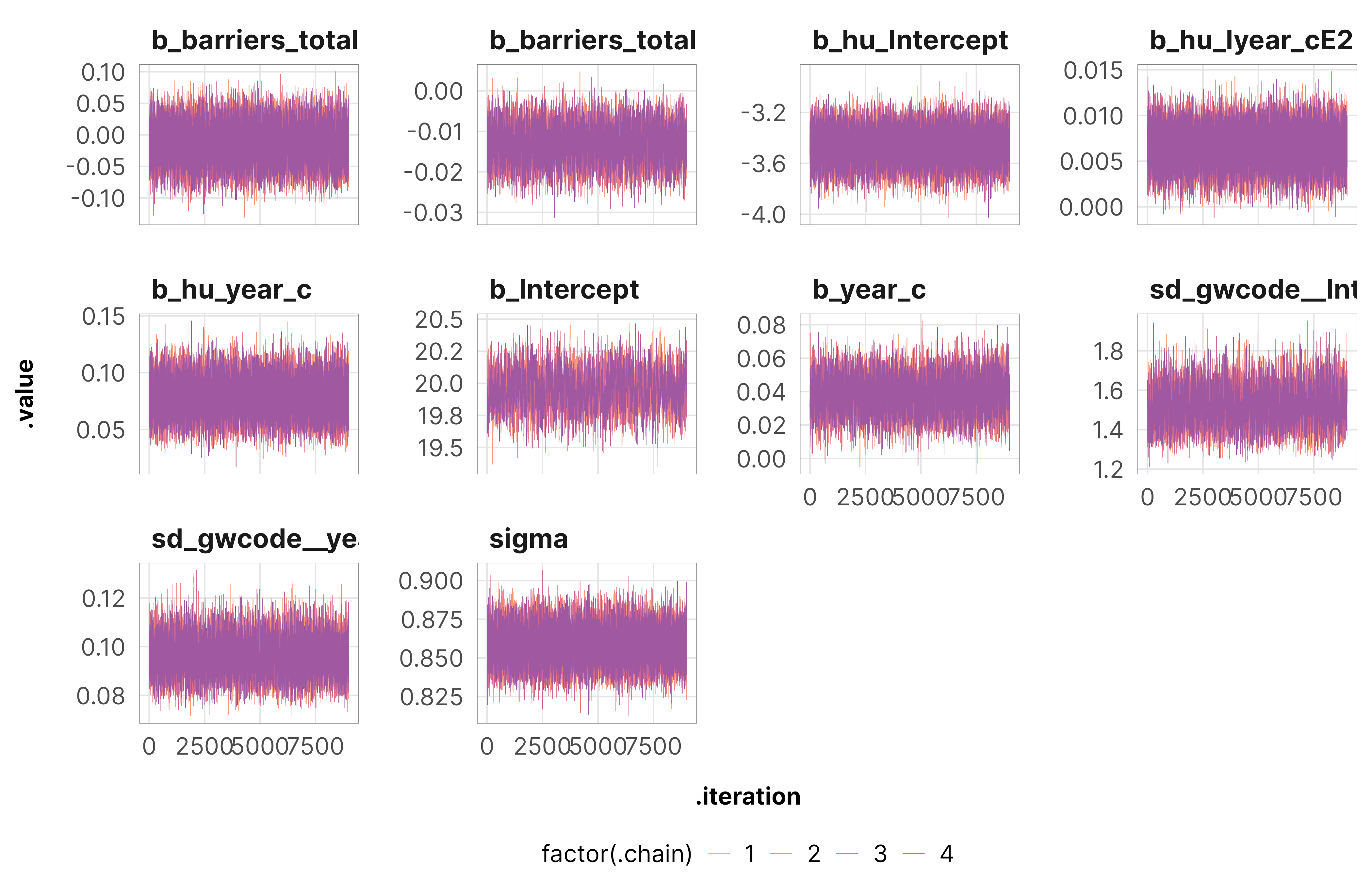
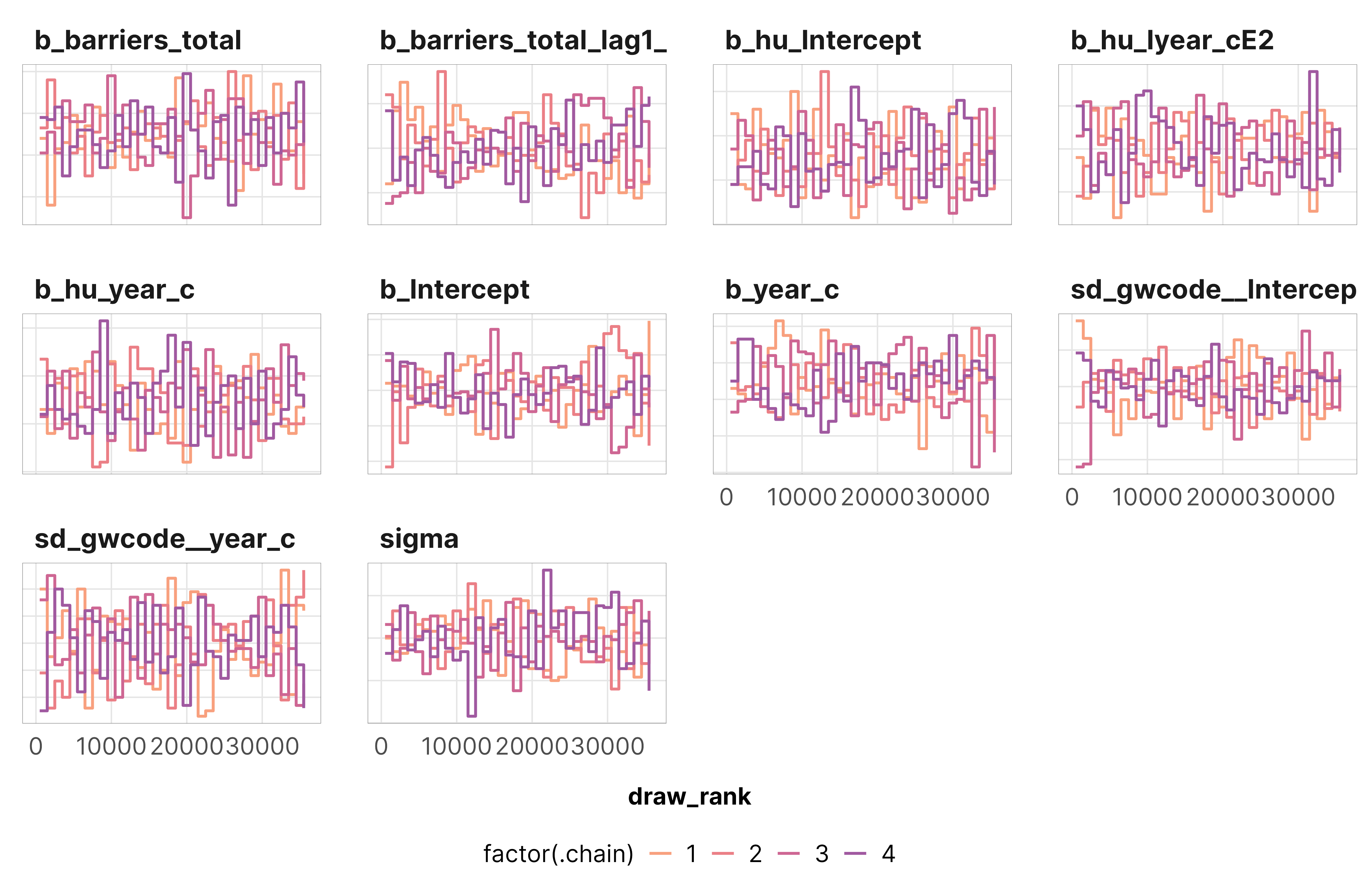
MCMC diagnostics
To check that everything converged nicely, we check some diagnostics for the outcome models for the total barriers treatment. All the other models look basically the same as this—everything’s fine.
In this project we care most about conditional effects, or the effect of the treatment in a typical country, or effect of the treatment when all country-specific \(b_0\) and \(b_3\) estimates are set to 0. That’s also what our main estimand is. We could also calculate marginal effects, or the effect of the treatment across all countries on average, which would require integrating out the random effects, but we’re most interested in the effect in a typical average country instead.
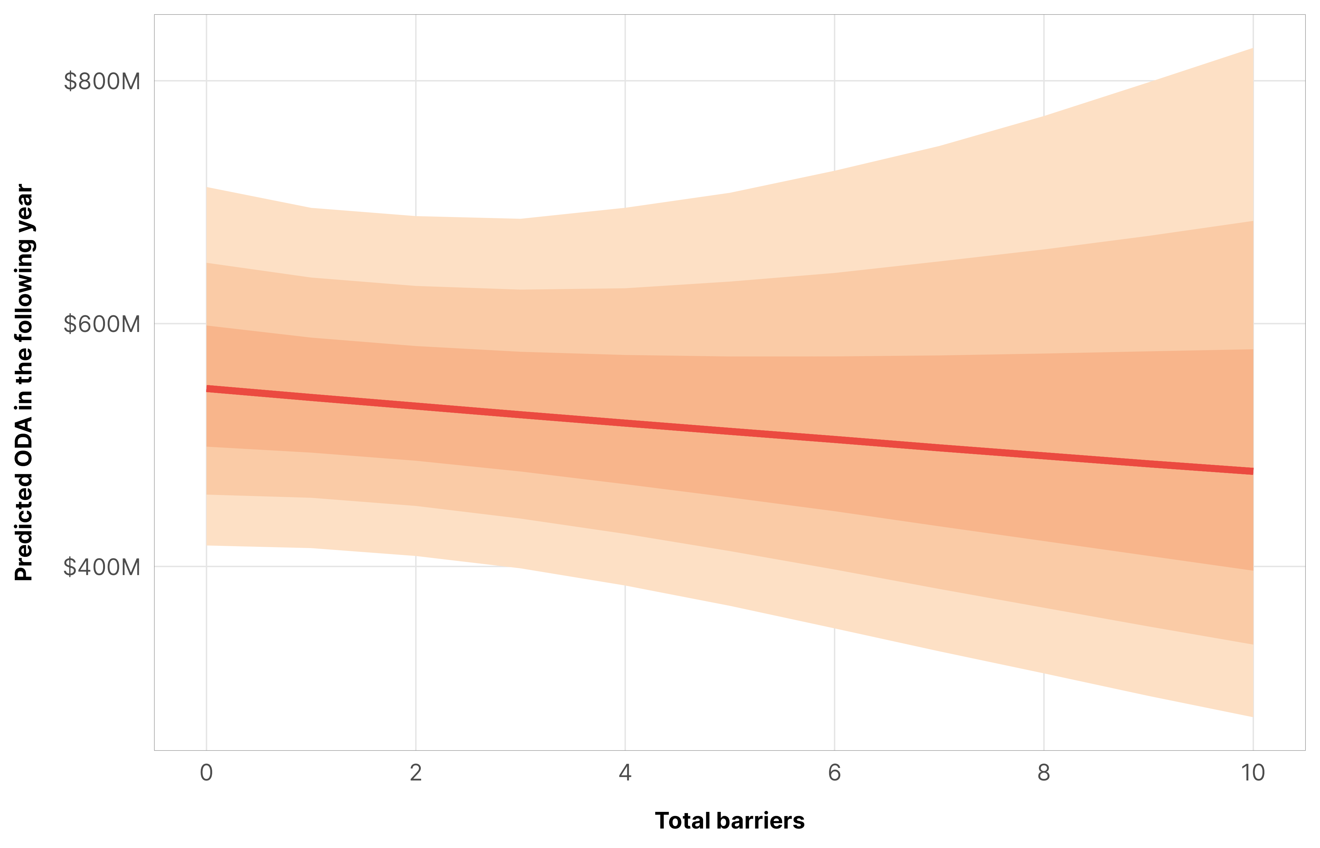
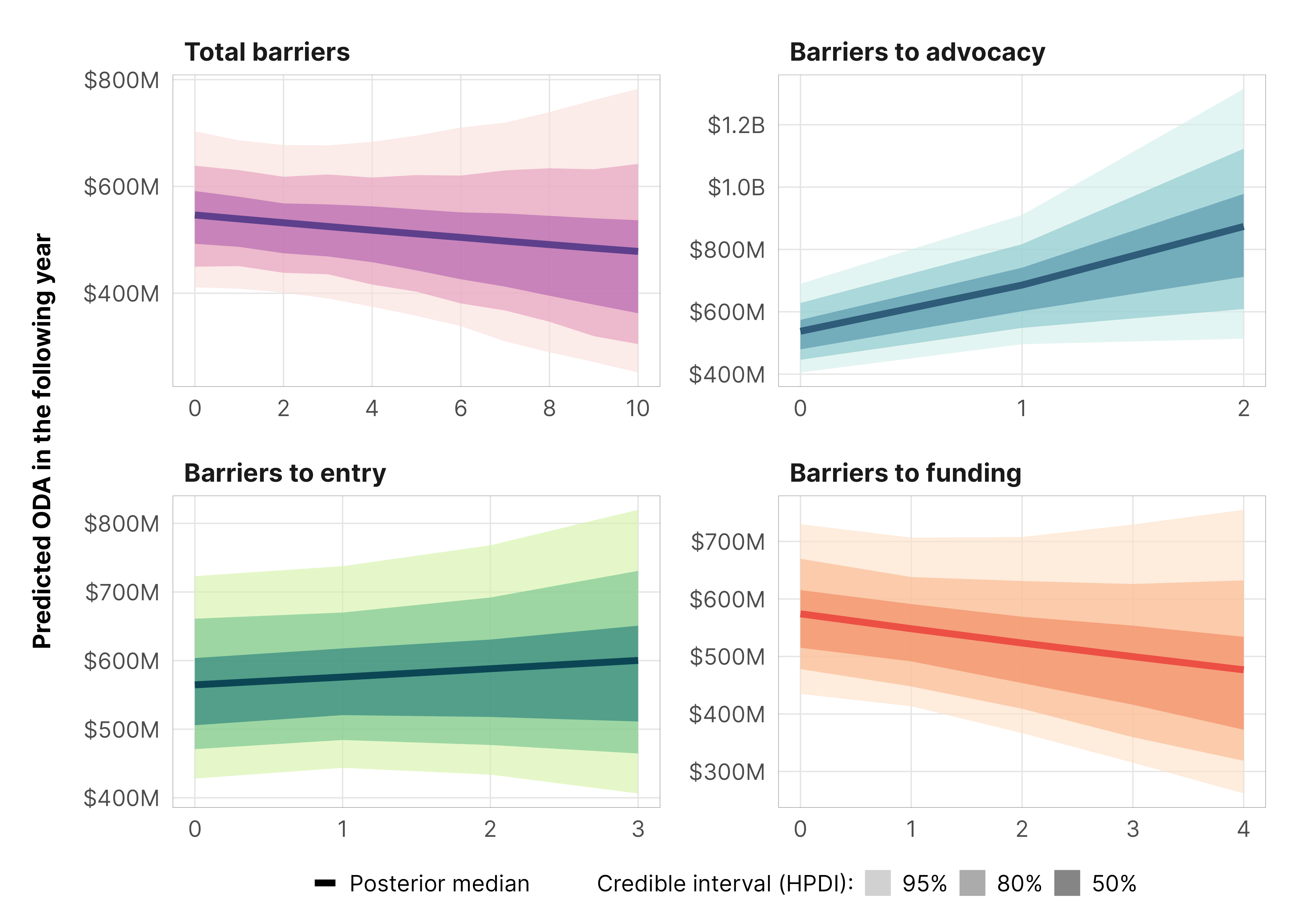
In general, aid decreases slightly as additional legal barriers are added:
Code
m_oda_outcome_total$model %>%epred_draws(newdata =datagrid(model = m_oda_outcome_total$model,year_c =0,barriers_total =seq(0, 10, 1)),re_formula =NA) %>%ggplot(aes(x = barriers_total, y = .epred)) +stat_lineribbon(color = clrs$Peach[7]) +scale_x_continuous(breaks =seq(0, 10, by =2)) +scale_y_continuous(labels =label_dollar(scale_cut =cut_short_scale())) +scale_fill_manual(values = clrs$Peach[1:3]) +guides(fill ="none") +labs(x ="Total barriers", y ="Predicted ODA in the following year") +theme_donors()
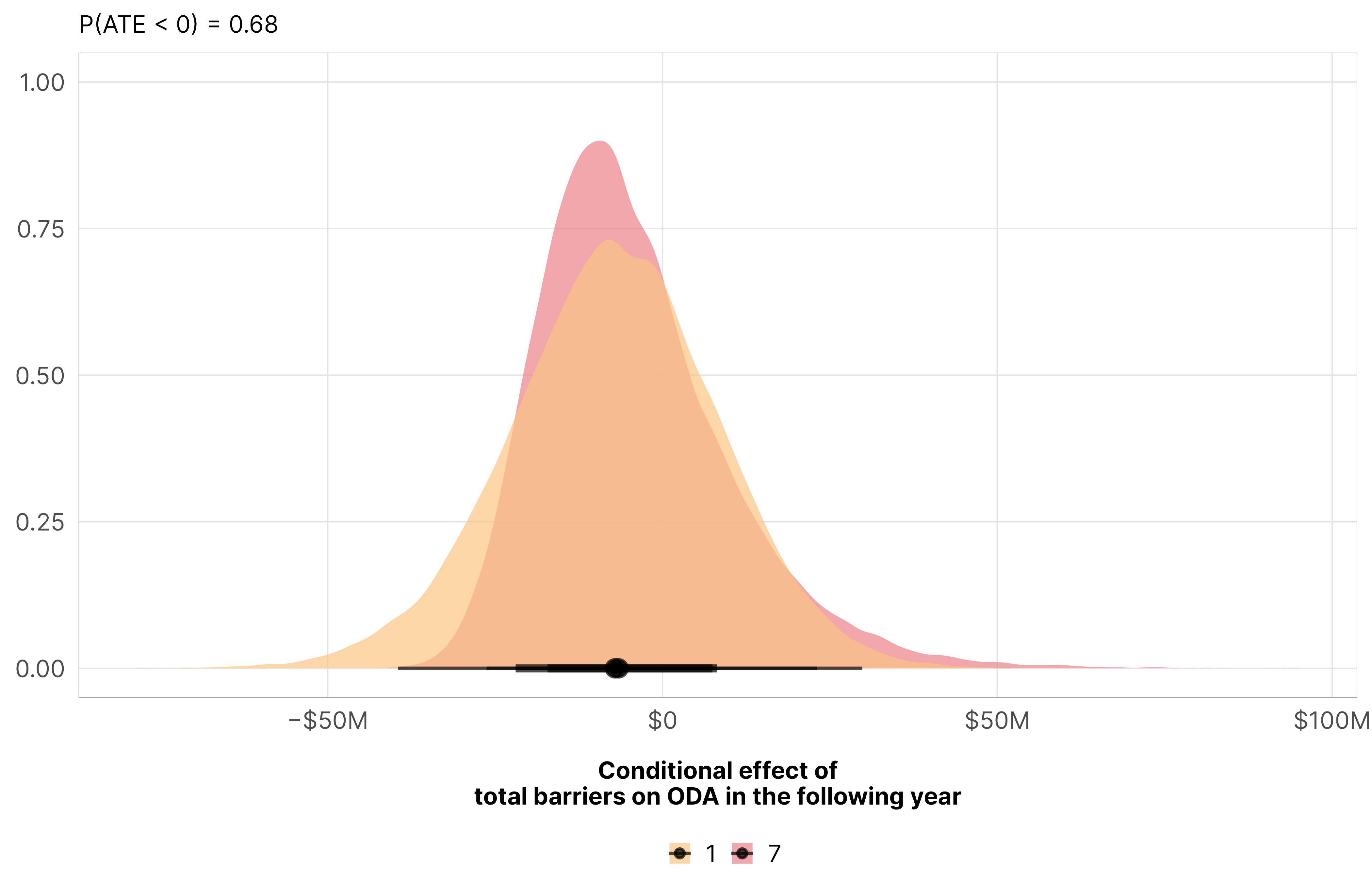
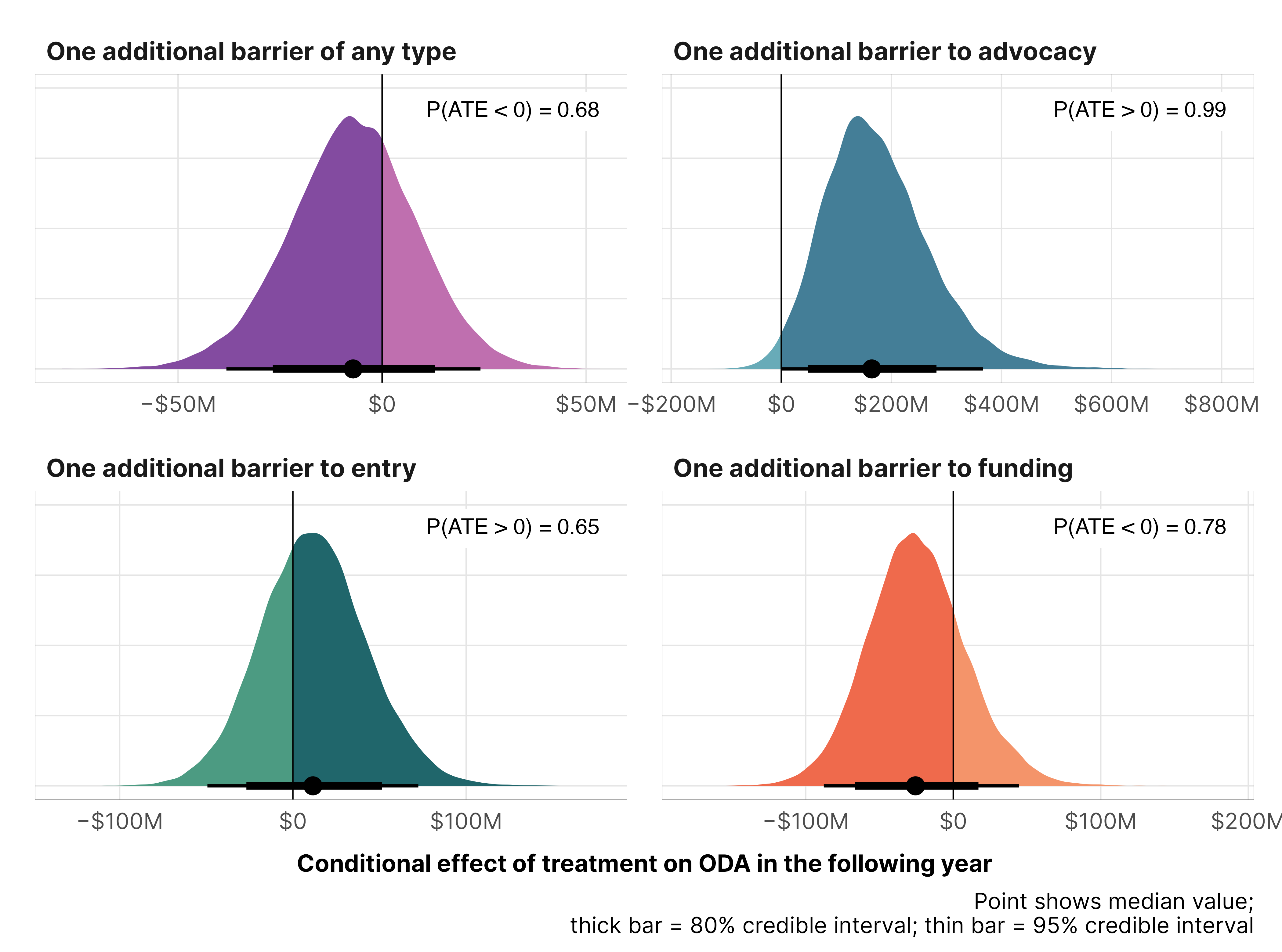
We can get the exact slope of the line at different levels of de jure restriction. The effect is fairly small—only a posterior median decrease of ≈$6 million, with pretty huge credible intervals
mfx_oda_cfx_multiple$total %>%posteriordraws() %>%filter(barriers_total %in%c(1, 7)) %>%pivot_longer(draw) %>%ggplot(aes(x = value, fill =factor(barriers_total))) +stat_halfeye(alpha =0.7) +scale_x_continuous(labels =label_dollar(style_negative ="minus", scale_cut =cut_short_scale())) +scale_fill_manual(values = clrs$Sunset[c(2, 4, 6)]) +labs(x ="Conditional effect of\ntotal barriers on ODA in the following year", y =NULL,subtitle =glue("P(ATE < 0) = {pull(mfx_total_p_direction, pd_short)}"), fill =NULL) +theme_donors()
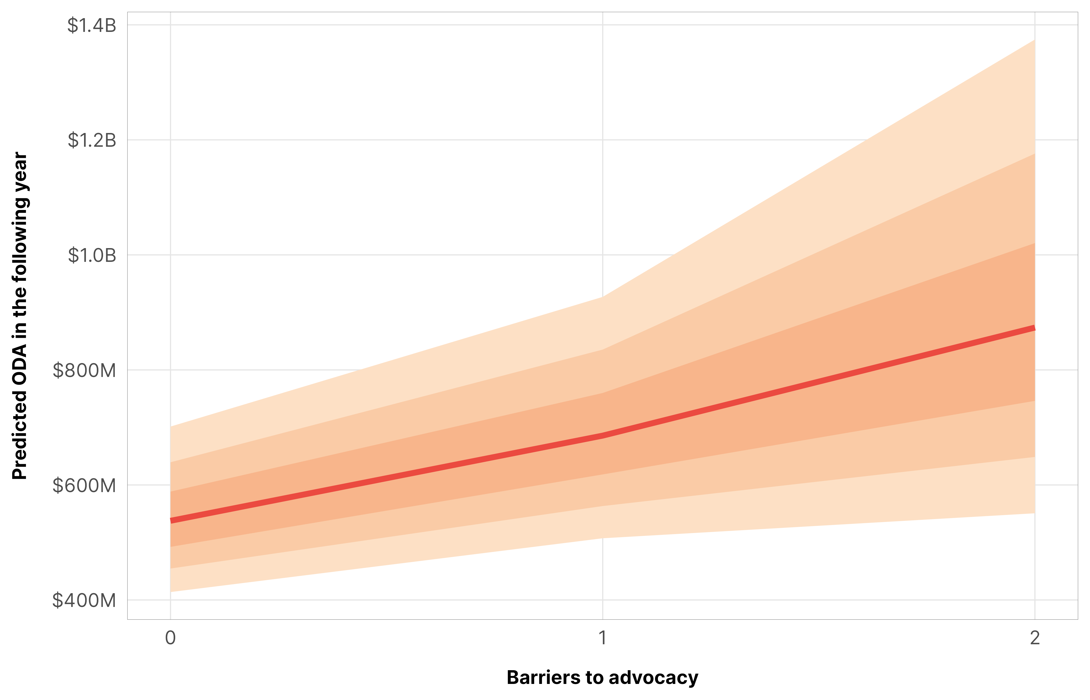
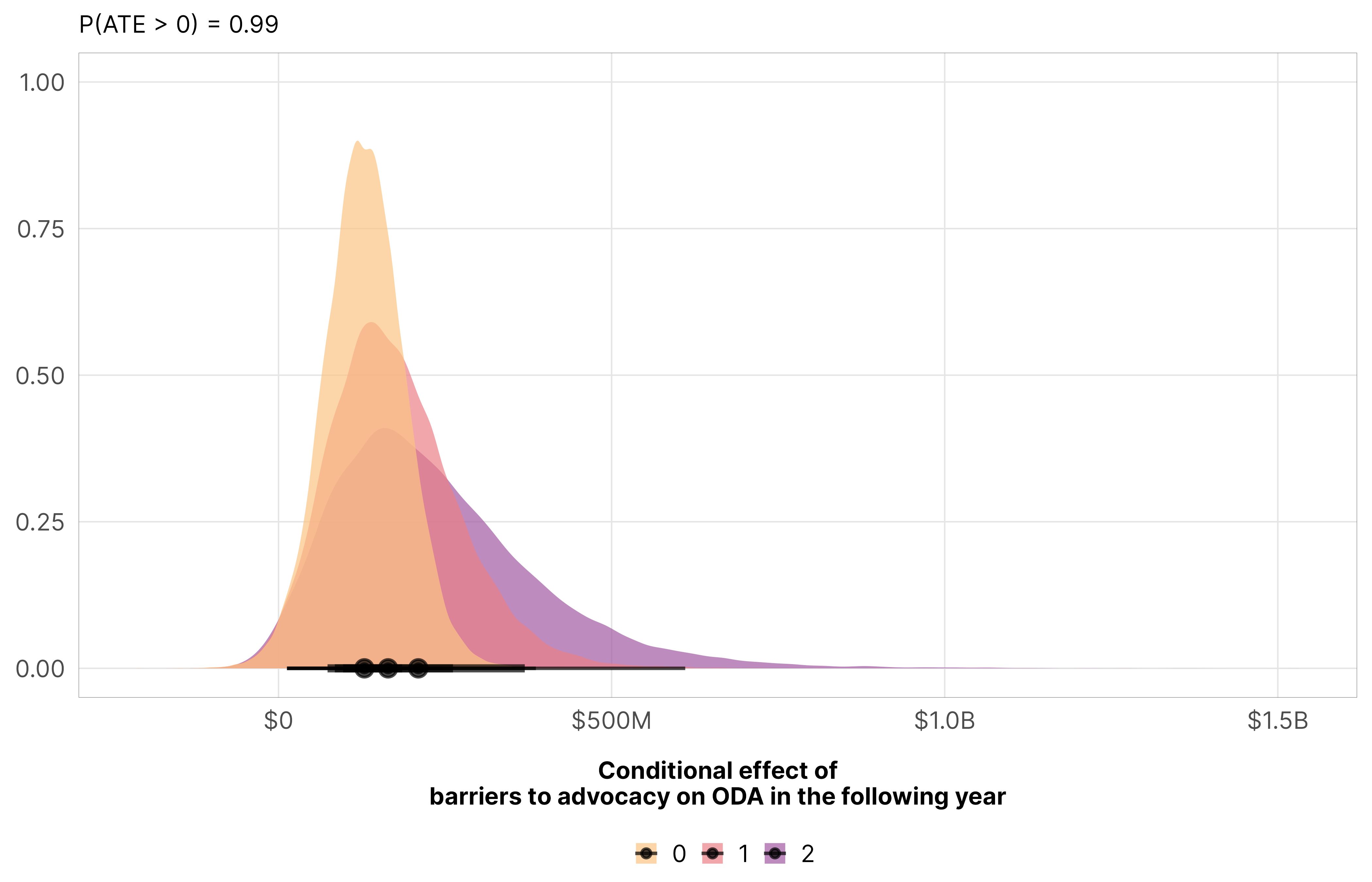
Here, total ODA increases significantly and substantially with the addition of new barriers to advocacy, with an increase of $130 to $200 million more ODA, depending on the initial count of legal barriers. Moving from 1 to 2 represents a 24% increase in aid.
Code
m_oda_outcome_advocacy$model %>%epred_draws(newdata =datagrid(model = m_oda_outcome_advocacy$model,year_c =0,advocacy =seq(0, 2, 1)),re_formula =NA) %>%ggplot(aes(x = advocacy, y = .epred)) +stat_lineribbon(color = clrs$Peach[7]) +scale_x_continuous(breaks =0:2) +scale_y_continuous(labels =label_dollar(scale_cut =cut_short_scale())) +scale_fill_manual(values = clrs$Peach[1:3]) +guides(fill ="none") +labs(x ="Barriers to advocacy", y ="Predicted ODA in the following year") +theme_donors()
mfx_oda_cfx_multiple$advocacy %>%posteriordraws() %>%pivot_longer(draw) %>%ggplot(aes(x = value, fill =factor(advocacy))) +stat_halfeye(alpha =0.7) +scale_x_continuous(labels =label_dollar(style_negative ="minus", scale_cut =cut_short_scale())) +scale_fill_manual(values = clrs$Sunset[c(2, 4, 6)]) +labs(x ="Conditional effect of\nbarriers to advocacy on ODA in the following year", y =NULL,subtitle =glue("P(ATE > 0) = {pull(mfx_advocacy_p_direction, pd_short)}"), fill =NULL) +theme_donors()
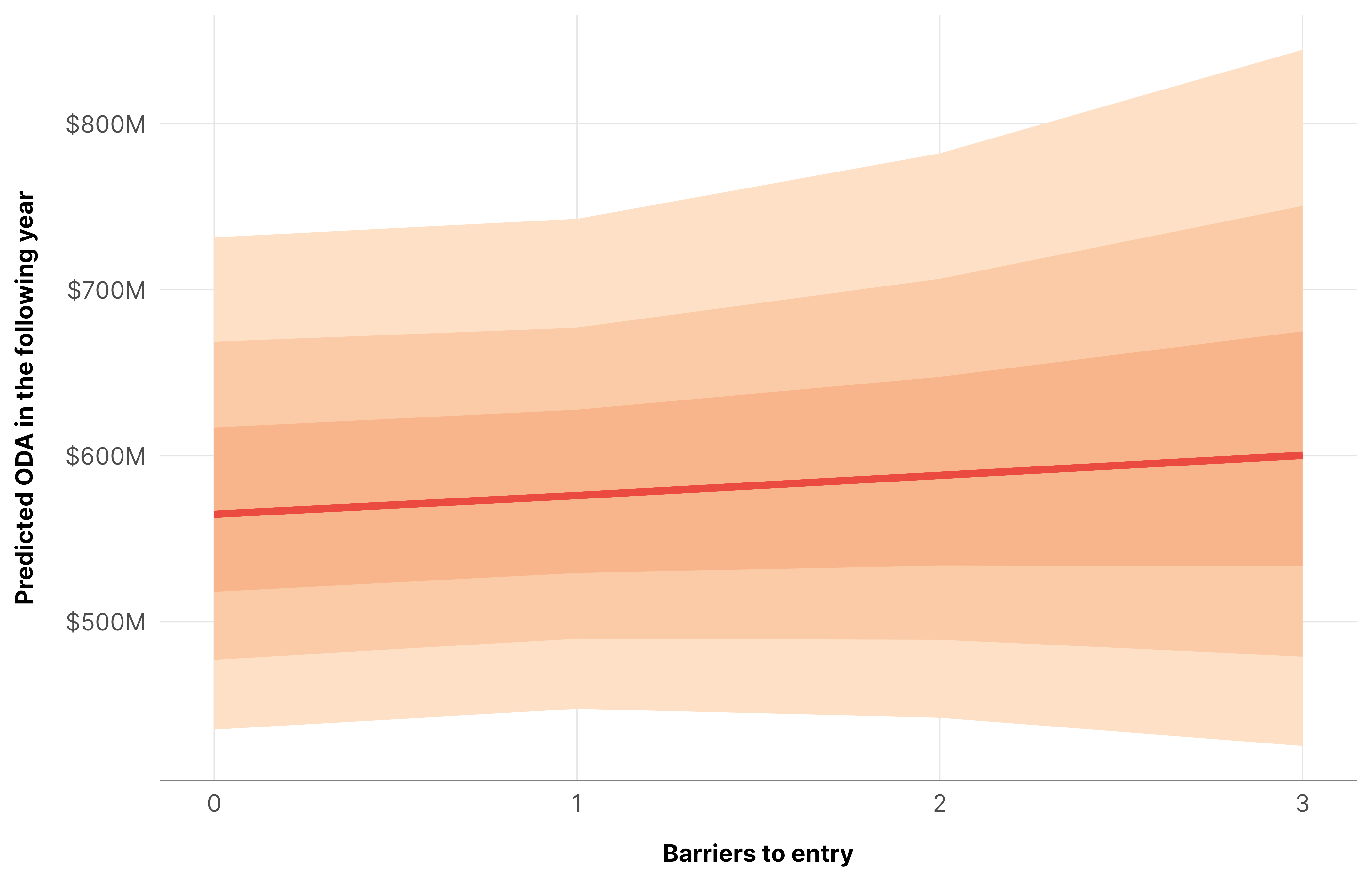
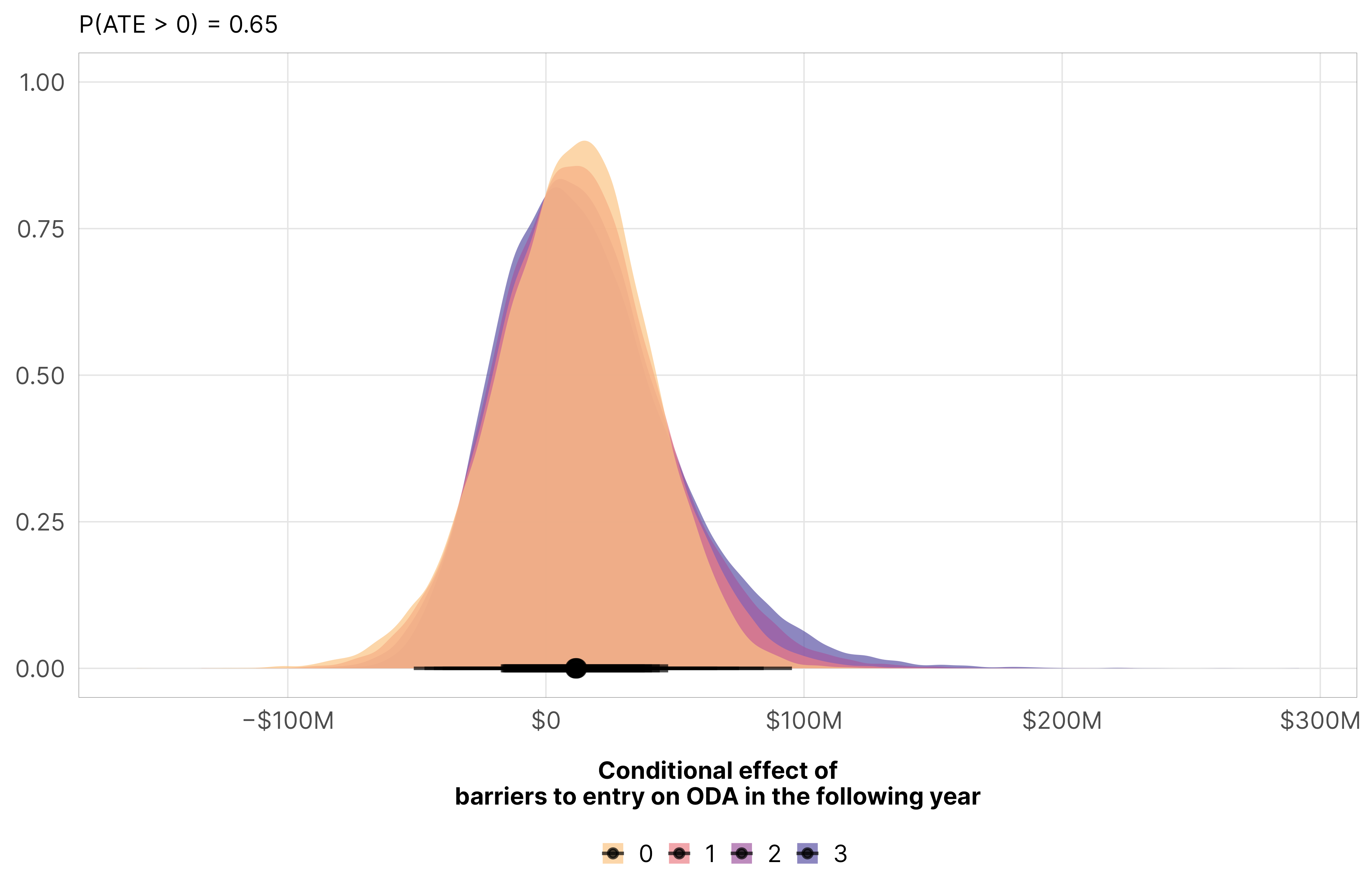
Adding additional barriers to entry doesn’t have much of an effect. It’s technically positive, but the probability that the slope is greater than zero is only 0.65.
Code
m_oda_outcome_entry$model %>%epred_draws(newdata =datagrid(model = m_oda_outcome_entry$model,year_c =0,entry =seq(0, 3, 1)),re_formula =NA) %>%ggplot(aes(x = entry, y = .epred)) +stat_lineribbon(color = clrs$Peach[7]) +scale_x_continuous(breaks =0:3) +scale_y_continuous(labels =label_dollar(scale_cut =cut_short_scale())) +scale_fill_manual(values = clrs$Peach[1:3]) +guides(fill ="none") +labs(x ="Barriers to entry", y ="Predicted ODA in the following year") +theme_donors()
mfx_oda_cfx_multiple$entry %>%posteriordraws() %>%pivot_longer(draw) %>%ggplot(aes(x = value, fill =factor(entry))) +stat_halfeye(alpha =0.7) +scale_x_continuous(labels =label_dollar(style_negative ="minus", scale_cut =cut_short_scale())) +scale_fill_manual(values = clrs$Sunset[c(2, 4, 6, 7)]) +labs(x ="Conditional effect of\nbarriers to entry on ODA in the following year", y =NULL,subtitle =glue("P(ATE > 0) = {pull(mfx_entry_p_direction, pd_short)}"), fill =NULL) +theme_donors()
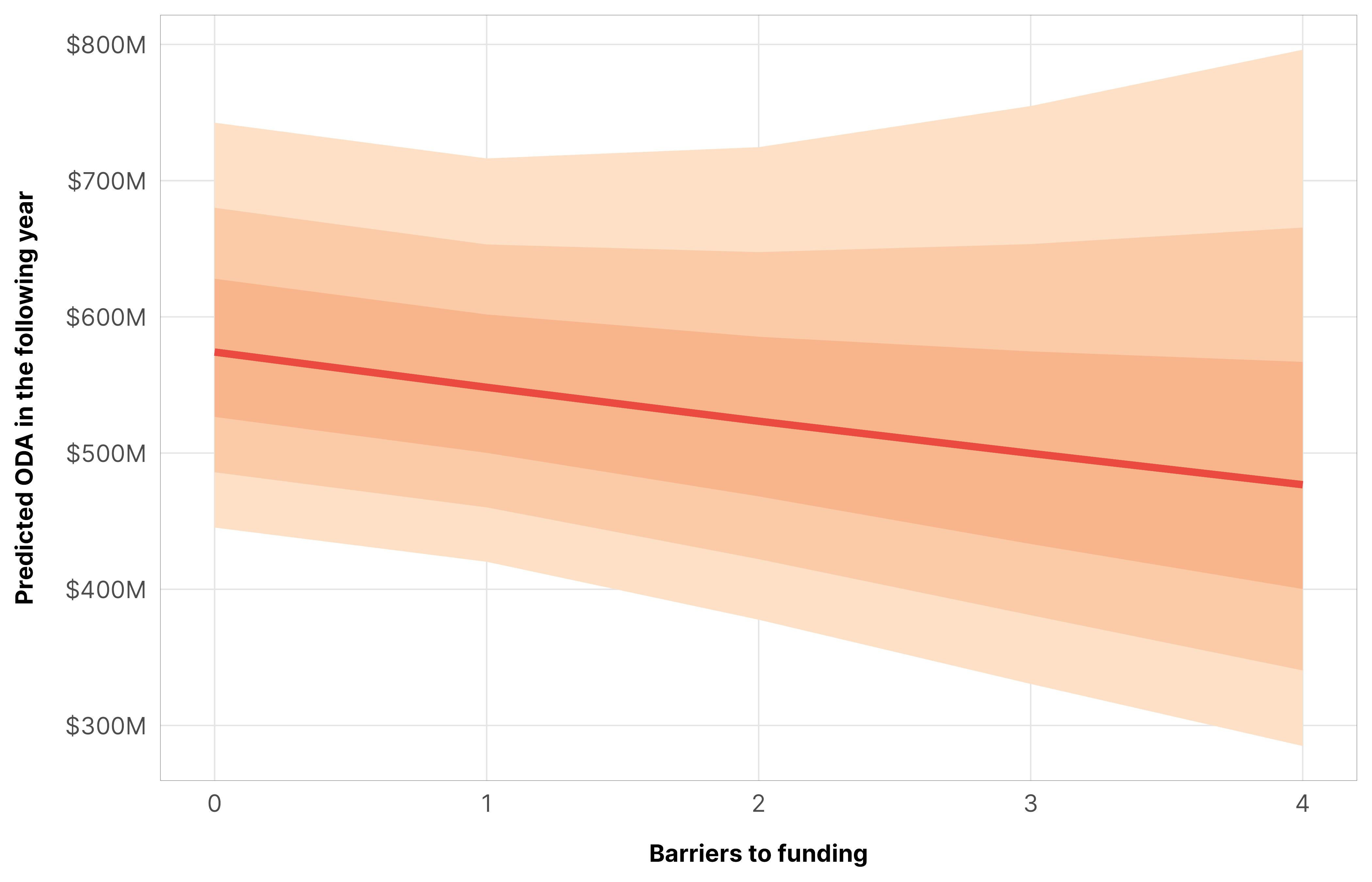
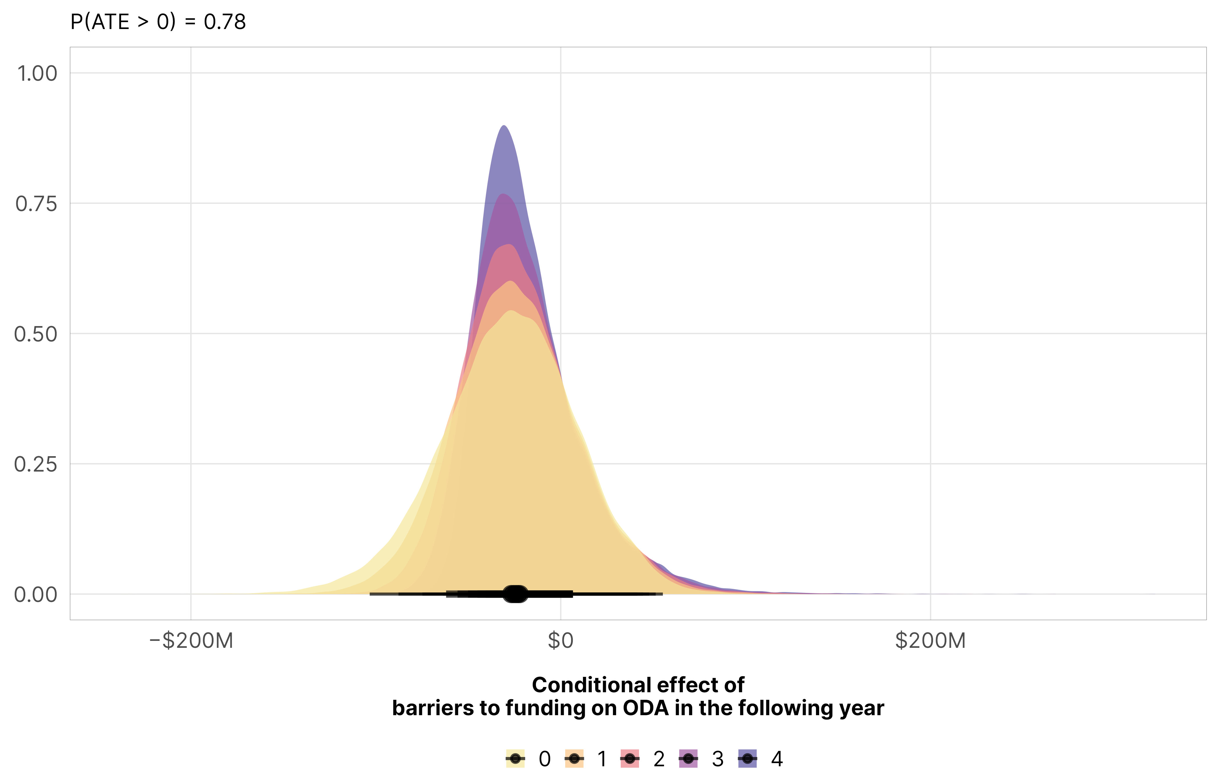
An additional barrier to funding leads to a 5ish% decrease in aid, but the probability that the decrease is negative is only 0.78.
Code
m_oda_outcome_funding$model %>%epred_draws(newdata =datagrid(model = m_oda_outcome_funding$model,year_c =0,funding =seq(0, 4, 1)),re_formula =NA) %>%ggplot(aes(x = funding, y = .epred)) +stat_lineribbon(color = clrs$Peach[7]) +scale_x_continuous(breaks =0:4) +scale_y_continuous(labels =label_dollar(scale_cut =cut_short_scale())) +scale_fill_manual(values = clrs$Peach[1:3]) +guides(fill ="none") +labs(x ="Barriers to funding", y ="Predicted ODA in the following year") +theme_donors()
mfx_oda_cfx_multiple$funding %>%posteriordraws() %>%pivot_longer(draw) %>%ggplot(aes(x = value, fill =factor(funding))) +stat_halfeye(alpha =0.7) +scale_x_continuous(labels =label_dollar(style_negative ="minus", scale_cut =cut_short_scale())) +scale_fill_manual(values = clrs$Sunset[c(1, 2, 4, 6, 7)]) +labs(x ="Conditional effect of\nbarriers to funding on ODA in the following year", y =NULL,subtitle =glue("P(ATE > 0) = {pull(mfx_funding_p_direction, pd_short)}"), fill =NULL) +theme_donors()
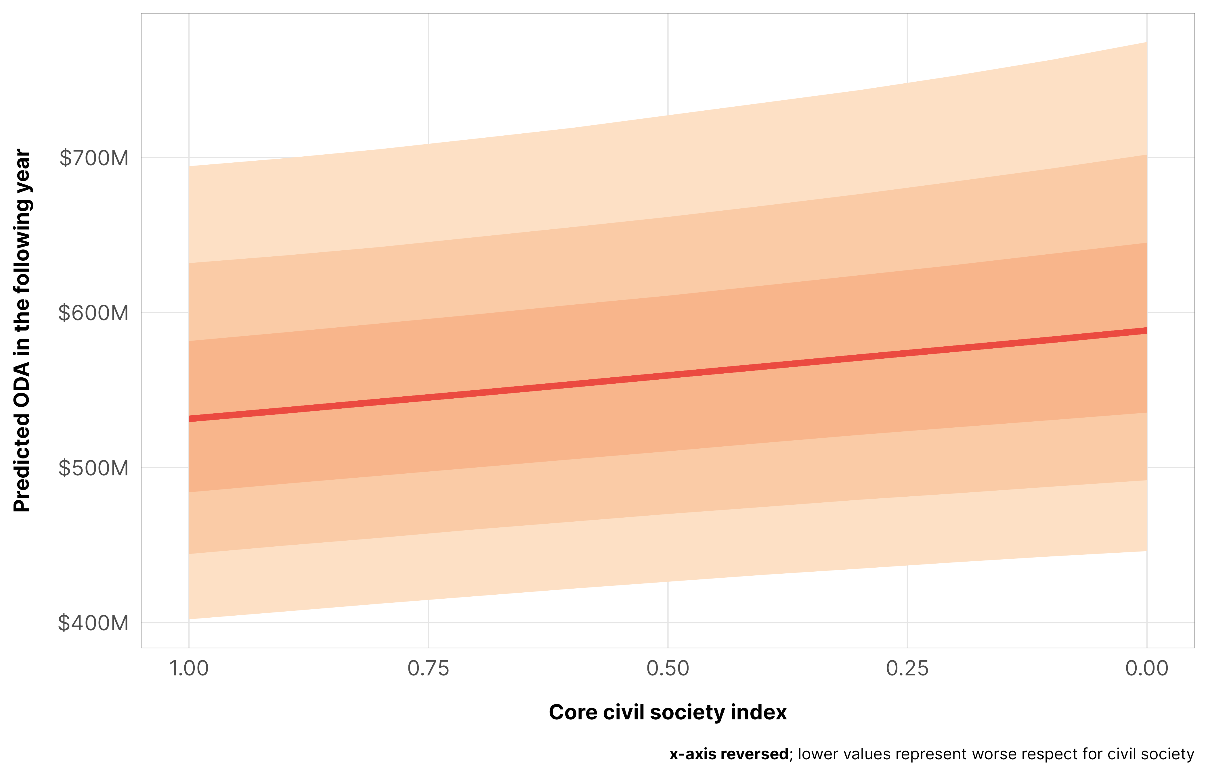
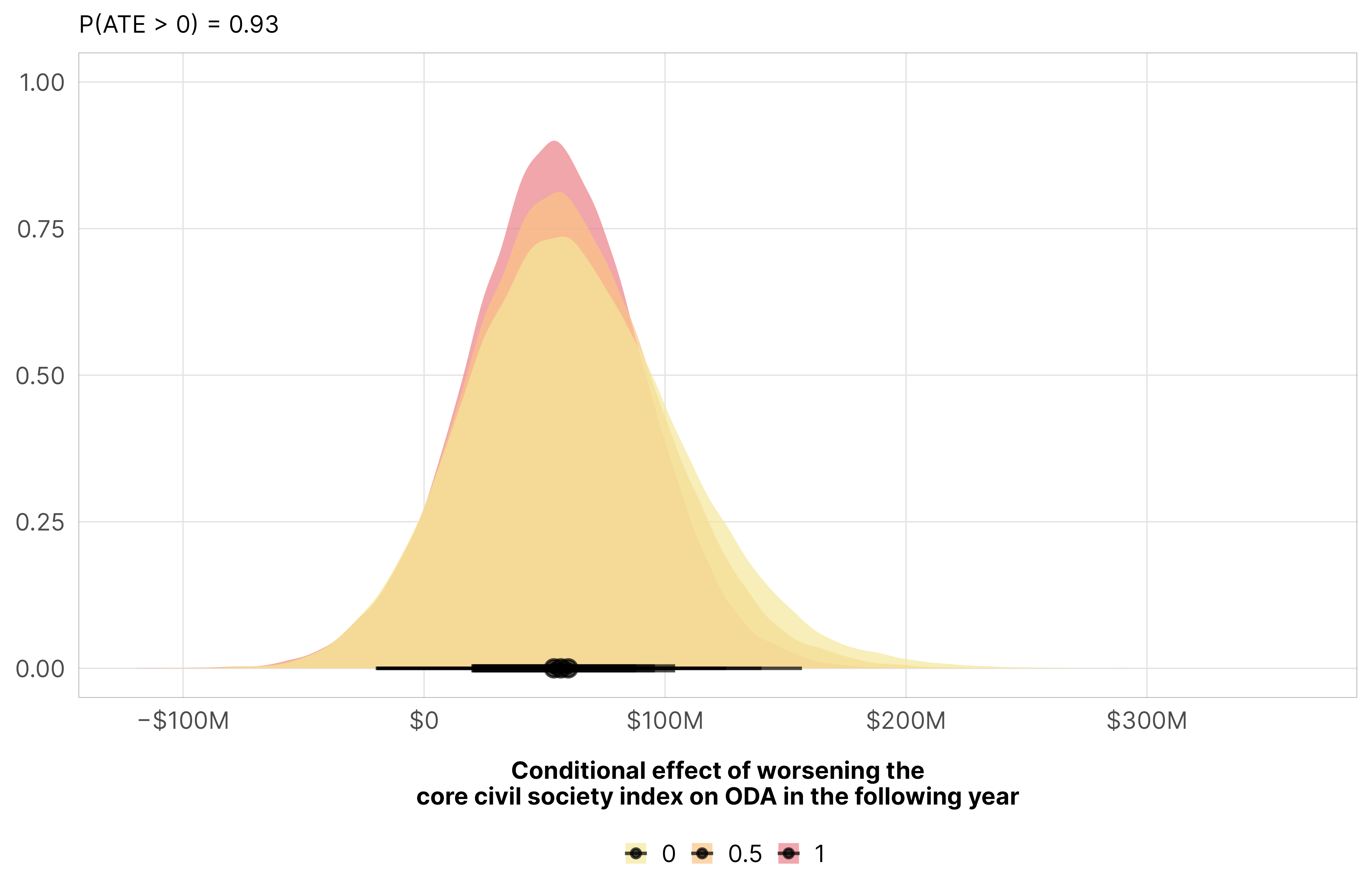
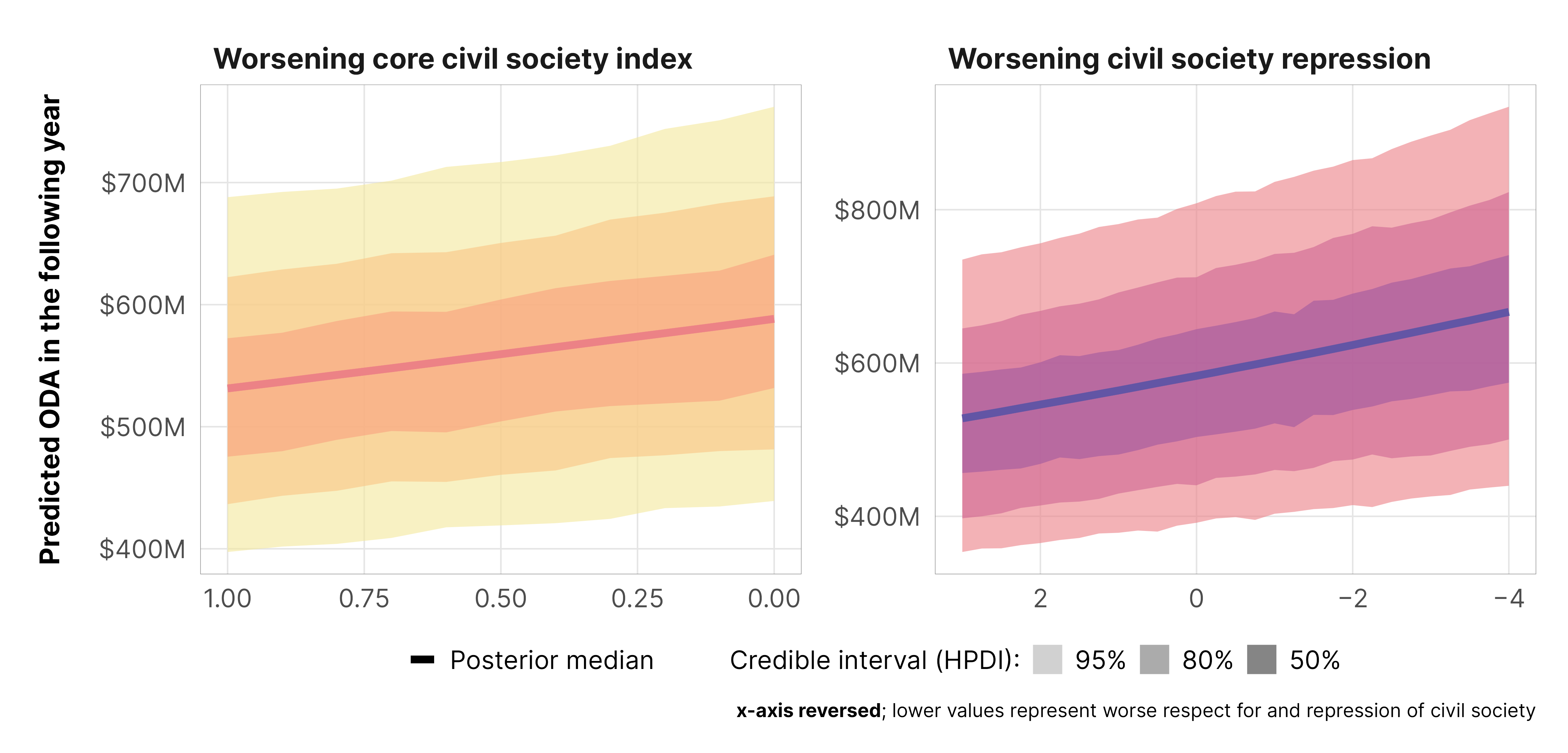
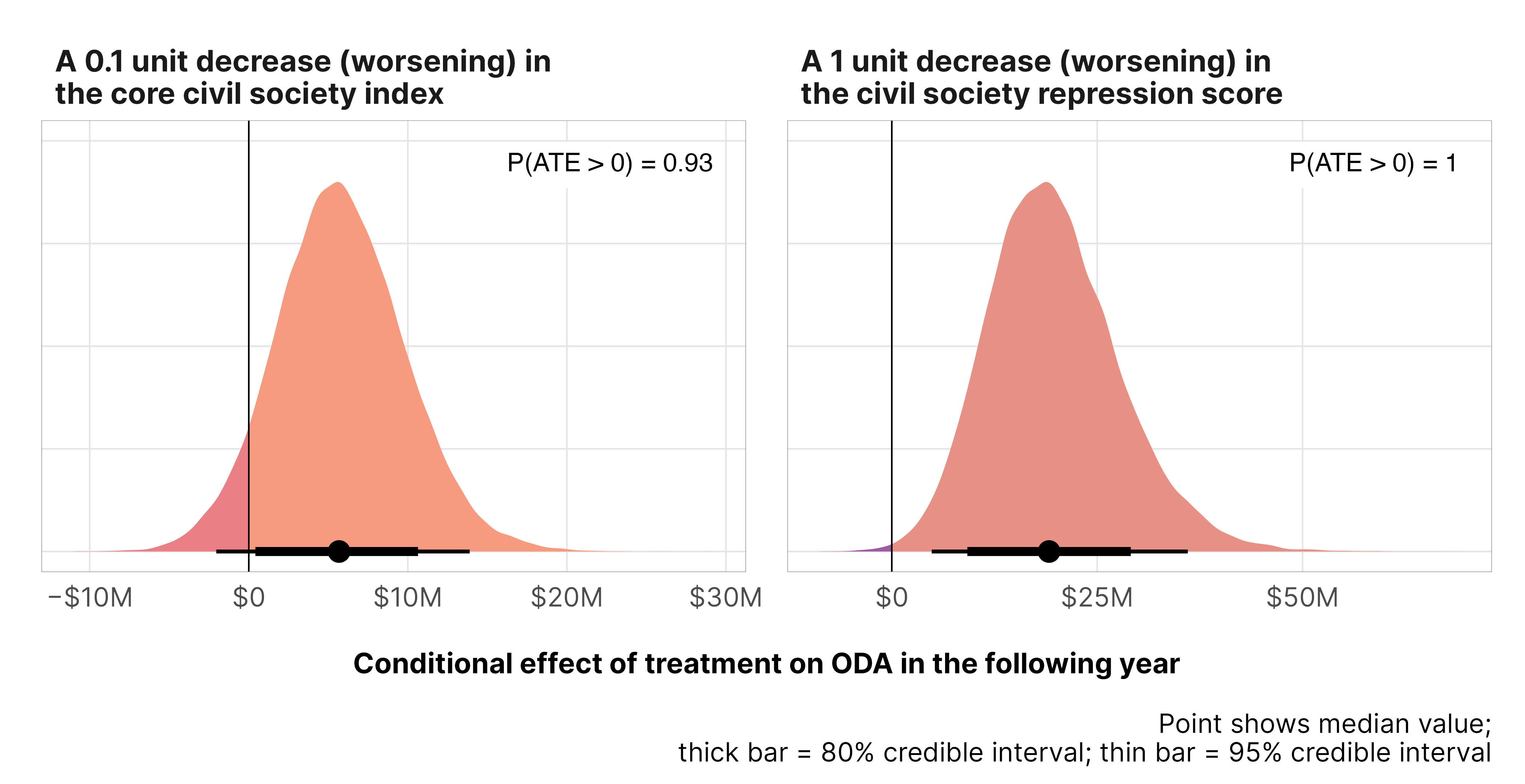
Improvements in the core civil society index lead to a tiny decrease in aid (a 1% drop, on average), and the probability that the effect is negative is 0.93. This is not an issue of punishment—donor countries aren’t withholding aid as countries improve. Instead, it’s helpful to think of this in reverse—as civil society gets worse in a country, aid increases a tiny bit.
Code
m_oda_outcome_ccsi$model_50 %>%epred_draws(newdata =datagrid(model = m_oda_outcome_ccsi$model_50,year_c =0,v2xcs_ccsi =seq(0, 1, 0.1)),re_formula =NA) %>%ggplot(aes(x = v2xcs_ccsi, y = .epred)) +stat_lineribbon(color = clrs$Peach[7]) +scale_x_reverse() +scale_y_continuous(labels =label_dollar(scale_cut =cut_short_scale())) +scale_fill_manual(values = clrs$Peach[1:3]) +guides(fill ="none") +labs(x ="Core civil society index", y ="Predicted ODA in the following year",caption ="**x-axis reversed**; lower values represent worse respect for civil society") +theme_donors() +theme(plot.caption =element_markdown())
mfx_oda_cfx_multiple$ccsi %>%posteriordraws() %>%mutate(draw =-draw) %>%pivot_longer(draw) %>%ggplot(aes(x = value, fill =factor(v2xcs_ccsi))) +stat_halfeye(alpha =0.7) +scale_x_continuous(labels =label_dollar(style_negative ="minus", scale_cut =cut_short_scale())) +scale_fill_manual(values = clrs$Sunset[c(1, 2, 4, 6, 7)]) +labs(x ="Conditional effect of worsening the\ncore civil society index on ODA in the following year", y =NULL,subtitle =glue("P(ATE > 0) = {pull(mfx_ccsi_p_direction, pd_short)}"), fill =NULL) +theme_donors()
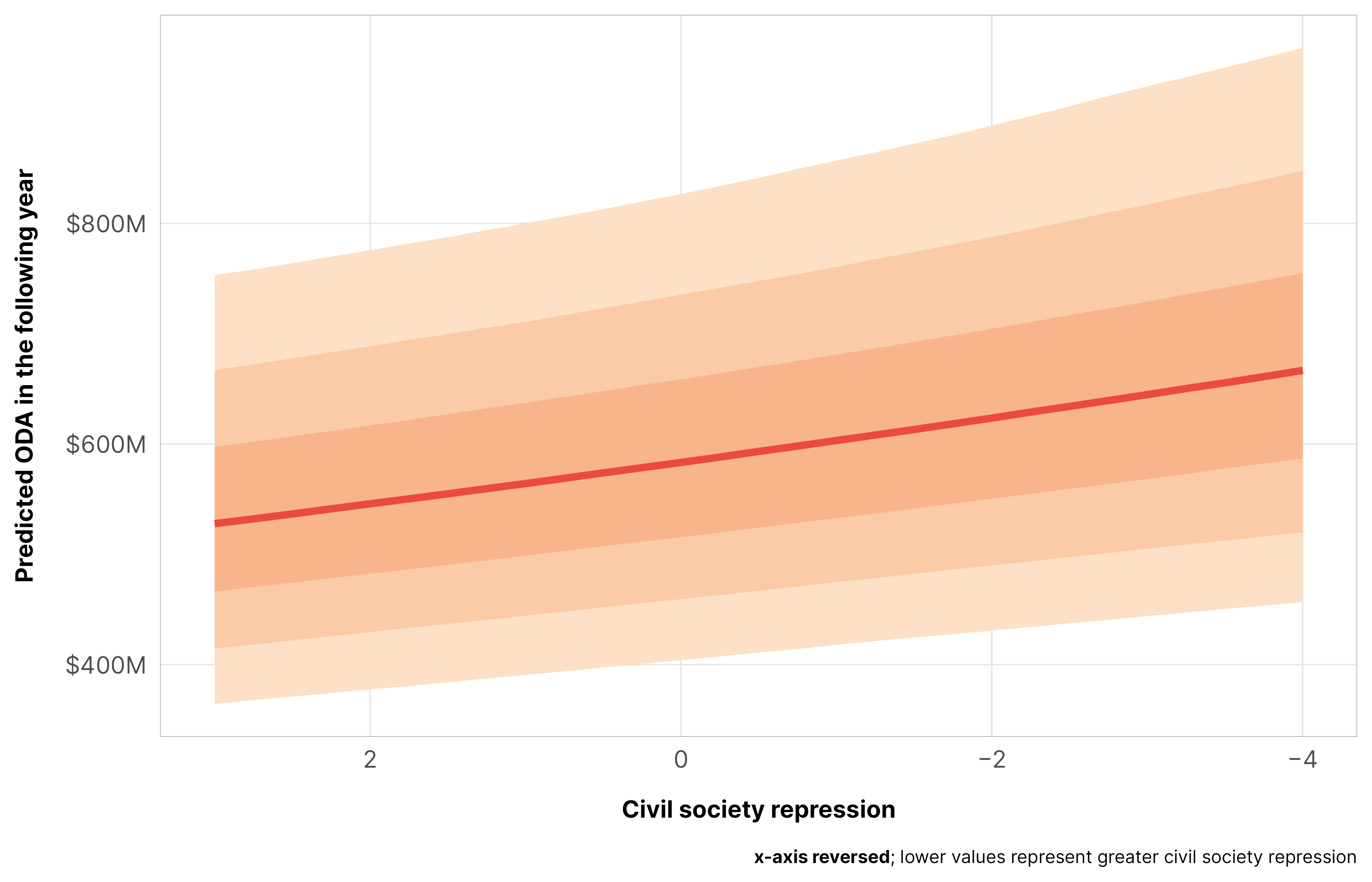
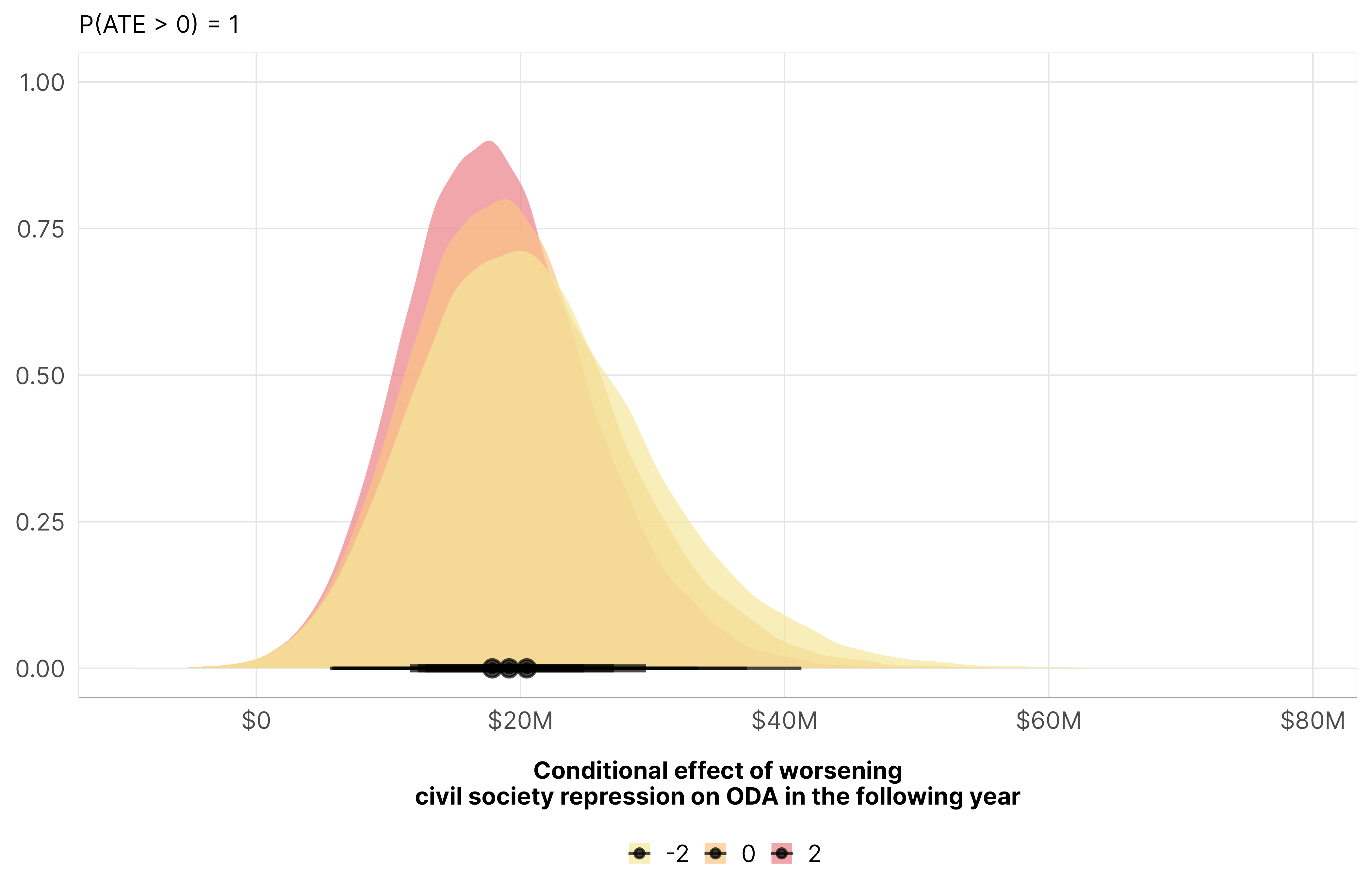
If we look at civil society repression in particular, we see the same effect. Improvements in civil society repression lead to 3% less aid (with p = 1 that it’s negative), or in reverse, more civil society repression leads to more aid. This is likely driven by the barriers to advocacy that we saw earlier.
Code
m_oda_outcome_repress$model_50 %>%epred_draws(newdata =datagrid(model = m_oda_outcome_repress$model_50,year_c =0,v2csreprss =seq(-4, 3, 0.25)),re_formula =NA) %>%ggplot(aes(x = v2csreprss, y = .epred)) +stat_lineribbon(color = clrs$Peach[7]) +scale_x_reverse(labels =label_number(style_negative ="minus")) +scale_y_continuous(labels =label_dollar(scale_cut =cut_short_scale())) +scale_fill_manual(values = clrs$Peach[1:3]) +guides(fill ="none") +labs(x ="Civil society repression", y ="Predicted ODA in the following year",caption ="**x-axis reversed**; lower values represent greater civil society repression") +theme_donors() +theme(plot.caption =element_markdown())
mfx_oda_cfx_multiple$repress %>%posteriordraws() %>%mutate(draw =-draw) %>%pivot_longer(draw) %>%ggplot(aes(x = value, fill =factor(v2csreprss))) +stat_halfeye(alpha =0.7) +scale_x_continuous(labels =label_dollar(style_negative ="minus", scale_cut =cut_short_scale())) +scale_fill_manual(values = clrs$Sunset[c(1, 2, 4, 6, 7)]) +labs(x ="Conditional effect of worsening\ncivil society repression on ODA in the following year", y =NULL,subtitle =glue("P(ATE > 0) = {pull(mfx_repress_p_direction, pd_short)}"), fill =NULL) +theme_donors()
# Put the shared y-axis label in a separate plot and add it to the combined plot# https://stackoverflow.com/a/66778622/120898p_lab <-ggplot() +annotate(geom ="text", x =1, y =1, angle =90, size =3.3, fontface ="bold",label ="Predicted ODA in the following year") +coord_cartesian(clip ="off") +theme_void()(p_lab | ((p1 | p2) / (p3 | p4) +plot_layout(guides ="collect") +plot_annotation(theme =theme(legend.position ="bottom")))) +plot_layout(widths =c(0.05, 1))
The effect of de jure anti-NGO legal barriers on predicted levels of foreign aid in a typical country
Code
p1 <- m_oda_outcome_ccsi$model_50 %>%epred_draws(newdata =datagrid(model = m_oda_outcome_ccsi$model_50,year_c =0,v2xcs_ccsi =seq(0, 1, 0.1)),re_formula =NA) %>%ggplot(aes(x = v2xcs_ccsi, y = .epred)) +stat_lineribbon(aes(color ="Posterior median"), alpha =0.6, point_interval = median_hdci) +scale_x_reverse(breaks =seq(0, 1, by =0.25)) +scale_y_continuous(labels =label_dollar(scale_cut =cut_short_scale())) +scale_color_manual(values = clrs$Sunset[4],guide =guide_legend(order =1, override.aes =list(fill =NA, alpha =1, color ="black")) ) +scale_fill_manual(values = clrs$Sunset[c(1, 2, 3)], labels =function(x) label_percent()(as.numeric(x)),guide =guide_legend(order =2, override.aes =list(color =NA, fill = ci_cols)) ) +labs(x =NULL, y =NULL, color =NULL, fill ="Credible interval (HPDI):") +facet_wrap(vars("Worsening core civil society index")) +theme_donors() +theme(legend.margin =margin(l =7.5, r =7.5))p2 <- m_oda_outcome_repress$model_50 %>%epred_draws(newdata =datagrid(model = m_oda_outcome_repress$model_50,year_c =0,v2csreprss =seq(-4, 3, 0.25)),re_formula =NA) %>%ggplot(aes(x = v2csreprss, y = .epred)) +stat_lineribbon(aes(color ="Posterior median"), alpha =0.6, point_interval = median_hdci) +scale_x_reverse(labels =label_number(style_negative ="minus")) +scale_y_continuous(labels =label_dollar(scale_cut =cut_short_scale())) +scale_color_manual(values = clrs$Sunset[7],guide =guide_legend(order =1, override.aes =list(fill =NA, alpha =1, color ="black")) ) +scale_fill_manual(values = clrs$Sunset[c(4, 5, 6)], labels =function(x) label_percent()(as.numeric(x)),guide =guide_legend(order =2, override.aes =list(color =NA, fill = ci_cols)) ) +labs(x =NULL, y =NULL, color =NULL, fill ="Credible interval (HPDI):",caption ="**x-axis reversed**; lower values represent worse respect for and repression of civil society") +facet_wrap(vars("Worsening civil society repression")) +theme_donors() +theme(legend.margin =margin(l =7.5, r =7.5),plot.caption =element_markdown())p_lab <-ggplot() +annotate(geom ="text", x =1, y =1, angle =90, size =3.3, fontface ="bold",label ="Predicted ODA in the following year") +coord_cartesian(clip ="off") +theme_void()(p_lab | ((p1 | p2) +plot_layout(guides ="collect") +plot_annotation(theme =theme(legend.position ="bottom")))) +plot_layout(widths =c(0.05, 1))
The effect of the de facto civil society legal environment on predicted levels of foreign aid in a typical country
p_lab <-ggplot() +annotate(geom ="text", x =1, y =1, size =3.3, fontface ="bold",label ="Conditional effect of treatment on ODA in the following year") +coord_cartesian(clip ="off") +theme_void()(((p1 | p2) / (p3 | p4)) / p_lab) +plot_layout(heights =c(1, 1, 0.1)) +plot_annotation(caption ="Point shows median value;\nthick bar = 80% credible interval; thin bar = 95% credible interval",theme =theme(plot.caption =element_text(family ="Inter")))
The effect of one additional de jure anti-NGO legal barrier on foreign aid in a typical country
Code
p1 <- mfx_oda_cfx_single$ccsi %>%posteriordraws() %>%mutate(draw =-draw /10) %>%ggplot(aes(x = draw)) +stat_halfeye(aes(fill_ramp =after_stat(x <0)),fill = clrs$Sunset[4], .width =c(0.8, 0.95),point_interval = median_hdci) +geom_vline(xintercept =0, linewidth =0.25) +annotate(geom ="richtext", label =glue("P(ATE > 0) = {pull(mfx_ccsi_stats, pd_short)}"),x =Inf, y =Inf, hjust =1, vjust =1, size =3,label.color =NA, label.margin =unit(rep(0.5, 4), "lines")) +scale_x_continuous(labels =label_dollar(scale_cut =cut_short_scale(),style_negative ="minus")) +scale_fill_ramp_discrete(from = clrs$Sunset[3], guide ="none") +labs(x =NULL, y =NULL, fill =NULL) +facet_wrap(vars("A 0.1 unit decrease (worsening) in\nthe core civil society index")) +theme_donors() +theme(axis.text.y =element_blank())p2 <- mfx_oda_cfx_single$repress %>%posteriordraws() %>%mutate(draw =-draw) %>%ggplot(aes(x = draw)) +stat_halfeye(aes(fill_ramp =after_stat(x <0)),fill = clrs$Sunset[6], .width =c(0.8, 0.95),point_interval = median_hdci) +geom_vline(xintercept =0, linewidth =0.25) +annotate(geom ="richtext", label =glue("P(ATE > 0) = {pull(mfx_repress_stats, pd_short)}"),x =Inf, y =Inf, hjust =1, vjust =1, size =3,label.color =NA, label.margin =unit(rep(0.5, 4), "lines")) +scale_x_continuous(labels =label_dollar(scale_cut =cut_short_scale(),style_negative ="minus")) +scale_fill_ramp_discrete(from = clrs$Sunset[3], guide ="none") +labs(x =NULL, y =NULL, fill =NULL) +facet_wrap(vars("A 1 unit decrease (worsening) in\nthe civil society repression score")) +theme_donors() +theme(axis.text.y =element_blank())p_lab <-ggplot() +annotate(geom ="text", x =1, y =1, size =3.3, fontface ="bold",label ="Conditional effect of treatment on ODA in the following year") +coord_cartesian(clip ="off") +theme_void()((p1 | p2) / p_lab) +plot_layout(heights =c(1, 0.15)) +plot_annotation(caption ="Point shows median value;\nthick bar = 80% credible interval; thin bar = 95% credible interval",theme =theme(plot.caption =element_text(family ="Inter")))
The effect of changes in the de facto civil society legal environment on predicted levels of foreign aid in a typical country
Table
Because of how {marginaleffects} deals with link transformations, we can’t get log-scale marginal effects that incorporate the hurdle process—the only way to incorporate hurdling is to use type = "response", which uses posterior_epred() behind the scenes, which returns values on the dollar scale. This isn’t {marginaleffects}’s fault, since posterior_epred() is the only way to get simultaneous results from both the non-hurdled and hurdled parts (since it’s the average of the full posterior prediction, or \(\textbf{E}[\operatorname{Hurdle\,log-normal}(\pi_{it}, \mu_{it_j}, \sigma_y)]\)), and it only returns values on the original response scale.
That’s great, but it can also be helpful to think of percent changes (especially with these multi-million dollar values!). Fortunately we can find percent changes pretty easily with calculus:
\[
\text{\% change when $x$ is $a$} = \frac{f'(x \mid x = a)}{f(x \mid x = a)}
\]
Code
signif_millions <-label_dollar(accuracy =1,prefix ="\\$",style_negative ="minus",scale_cut =cut_short_scale())signif_pct <-label_percent(accuracy =0.1,style_negative ="minus")mfx_lookup <-tribble(~term, ~Treatment,"barriers_total", "One additional barrier of any type","advocacy", "One additional barrier to advocacy","entry", "One additional barrier to entry","funding", "One additional barrier to funding","v2xcs_ccsi", "A 0.1 unit decrease in the core civil society index (i.e. worse environment)","v2csreprss", "A 1 unit decrease in the civil society repression score (i.e. more repression)") %>%mutate(Treatment =fct_inorder(Treatment))mfx_all_posteriors <-bind_rows(posteriordraws(mfx_oda_cfx_single$total), posteriordraws(mfx_oda_cfx_single$advocacy), posteriordraws(mfx_oda_cfx_single$entry), posteriordraws(mfx_oda_cfx_single$funding), (posteriordraws(mfx_oda_cfx_single$ccsi) %>%mutate(draw = draw /10)),posteriordraws(mfx_oda_cfx_single$repress)) %>%mutate(draw =ifelse(term %in%c("v2xcs_ccsi", "v2csreprss"), -draw, draw),dydx =ifelse(term %in%c("v2xcs_ccsi", "v2csreprss"), -dydx, dydx),conf.low_real =ifelse(term %in%c("v2xcs_ccsi", "v2csreprss"), -conf.high, conf.low),conf.high_real =ifelse(term %in%c("v2xcs_ccsi", "v2csreprss"), -conf.low, conf.high),conf.low = conf.low_real, conf.high = conf.high_real)mfx_p_direction <- mfx_all_posteriors %>%group_by(term) %>%summarize(pd_lt =round(sum(draw <0) /n(), 2),pd_gt =round(sum(draw >0) /n(), 2))mfx_medians <- mfx_all_posteriors %>%mutate(pct_change = draw / predicted) %>%group_by(term) %>%median_hdci(draw, pct_change) %>%left_join(mfx_p_direction, by ="term") %>%mutate(direction =case_when( draw >0~"more ODA in the next year", draw <0~"less ODA in the next year" )) %>%mutate(pd =case_when( draw >0~ pd_gt, draw <0~ pd_lt )) %>%mutate(pd_nice =label_percent(accuracy =1)(pd)) %>%mutate(across(c(draw, draw.lower, draw.upper), ~signif_millions(.))) %>%mutate(across(c(pct_change, pct_change.lower, pct_change.upper), ~signif_pct(.))) %>%mutate(draw.interval =glue("[{draw.lower}, {draw.upper}]")) %>%mutate(pct_change.interval =glue("[{pct_change.lower}, {pct_change.upper}]")) %>%mutate(draw.nice =glue("{draw}\n{draw.interval}"),pct_change.nice =glue("{pct_change}\n{pct_change.interval}")) %>%left_join(mfx_lookup, by ="term")mfx_medians_with_plots <- mfx_medians %>%group_by(term) %>%nest() %>%mutate(sparkplot =map(data, ~spark_bar(.x))) %>%mutate(sparkname =glue("sparkplots/oda_bar_{term}")) %>%mutate(saved_plot =map2(sparkplot, sparkname, ~save_sparks(.x, .y)))mfx_median_clean <- mfx_medians_with_plots %>%ungroup() %>%select(-sparkplot) %>%unnest_wider(saved_plot) %>%unnest(data) %>%arrange(Treatment)
Code
tbl_notes <-c("The probability denotes the percentage of the posterior distribution that falls above or below 0.","Reported values are the median posterior marginal effect of each treatment variable on the outcome, as millions of USD; 95% highest posterior density intervals (HPDI) shown in brackets.","The percent change value is calculated by dividing the marginal effect by the predicted value (or \\(f'(x \\mid x = a) / f(x \\mid x = a)\\)) when the count of legal barriers is set to 1 (i.e. one barrier to advocacy, one barrier to entry, etc.), when the core civil society index is set to 0.5, and when civil society repression is set to 0.")mfx_median_clean %>%mutate(Probability ="") %>%# mutate(across(c(draw.nice, pct_change.nice), ~linebreak(., align = "c"))) %>% # For LaTeXmutate(across(c(draw.nice, pct_change.nice), ~str_replace(., "\\n", "<br>"))) %>%select(Treatment, direction, Probability, draw.nice, pct_change.nice) %>%set_names(c("Countries that add…", "…receive…", paste0("Probability", footnote_marker_symbol(1)),paste0("Median", footnote_marker_symbol(2)), paste0("% change", footnote_marker_symbol(3)))) %>%kbl(align =c("l", "l", "c", "c", "c"), escape =FALSE) %>%kable_styling(htmltable_class ="table table-sm table-borderless") %>%pack_rows("De jure legislation", 1, 4, indent =FALSE) %>%pack_rows("De facto enforcement", 5, 6, indent =FALSE) %>%column_spec(1, width ="35%") %>%column_spec(2, width ="15%") %>%column_spec(3, image = mfx_median_clean$png, width ="14%") %>%column_spec(4, width ="18%") %>%column_spec(5, width ="18%") %>%footnote(symbol = tbl_notes, footnote_as_chunk =FALSE)
Countries that add…
…receive…
Probability*
Median†
% change‡
De jure legislation
One additional barrier of any type
less ODA in the next year
−\$7M [−\$38M, \$24M]
−1.3% [−7.1%, 4.5%]
One additional barrier to advocacy
more ODA in the next year
\$164M [−\$326K, \$366M]
24.0% [0.0%, 53.4%]
One additional barrier to entry
more ODA in the next year
\$12M [−\$49M, \$72M]
2.0% [−8.6%, 12.6%]
One additional barrier to funding
less ODA in the next year
−\$26M [−\$88M, \$45M]
−4.7% [−16.0%, 8.1%]
De facto enforcement
A 0.1 unit decrease in the core civil society index (i.e. worse environment)
more ODA in the next year
\$6M [−\$2M, \$14M]
1.0% [−0.4%, 2.5%]
A 1 unit decrease in the civil society repression score (i.e. more repression)
more ODA in the next year
\$19M [\$5M, \$36M]
3.3% [0.8%, 6.2%]
* The probability denotes the percentage of the posterior distribution that falls above or below 0.
† Reported values are the median posterior marginal effect of each treatment variable on the outcome, as millions of USD; 95% highest posterior density intervals (HPDI) shown in brackets.
‡ The percent change value is calculated by dividing the marginal effect by the predicted value (or \(f'(x \mid x = a) / f(x \mid x = a)\)) when the count of legal barriers is set to 1 (i.e. one barrier to advocacy, one barrier to entry, etc.), when the core civil society index is set to 0.5, and when civil society repression is set to 0.
Within- and between-country variability
The \(\sigma\) terms are roughly the same across all these different models, so we’ll just show the results from the total barriers model here. We have three \(\sigma\) terms to work with:
\(\sigma_y\) (sd__Observation): This is 0.858, which means that within any country, their total ODA varies by 0.9 logged units, so if their baseline is \(e^{19}\), their total aid will bounce around between \(e^{18.1}\) and \(e^{19.9}\).
\(\sigma_0\) (sd__(Intercept) for the gwcode group): This is the variability between countries’ baseline averages, or the variability around the \(b_{0_j}\) offsets. Here it’s 1.52, which means that across or between countries, total ODA varies by 1.5 logged units.
\(\sigma_3\) (sd__year_c for the gwcode group): the variability between countries’ year effects, or the variability around the \(b_{3_j}\) offsets. Here it’s 0.096, which means that average year effects vary by 10ish% across or between countries.
Again, this is less important since we don’t care about individual coefficients and instead care about conditional effects, but for the sake of full transparency (and to placate future reviewers), here’s a table of all the results:
Code
models_tbl_h1_outcome_dejure <- models_tbl_h1_outcome_dejure %>%set_names(1:length(.))notes <-c("Posterior medians; 95% credible intervals (HDPI) in brackets.", "Total \\(R^2\\) considers the variance of both population and group effects;", "marginal \\(R^2\\) only takes population effects into account")modelsummary(models_tbl_h1_outcome_dejure,estimate ="{estimate}",statistic ="[{conf.low}, {conf.high}]",add_rows = outcome_rows,coef_map = coefs_outcome,gof_map = gofs,output ="kableExtra",fmt =list(estimate =2, conf.low =2, conf.high =2)) %>%row_spec(1, bold =TRUE) %>%kable_styling(htmltable_class ="table-sm light-border") %>%footnote(general = notes, footnote_as_chunk =TRUE)
Table 4: Results from all outcome models
1
2
3
4
Treatment
Total barriers (t)
Barriers to advocacy (t)
Barriers to entry (t)
Barriers to funding (t)
Treatment (t − 1)
−0.01
0.24
0.02
−0.05
[−0.07, 0.04]
[0.02, 0.46]
[−0.08, 0.12]
[−0.17, 0.07]
Treatment history
−0.01
−0.04
−0.02
−0.02
[−0.02, −0.005]
[−0.07, −0.02]
[−0.03, −0.002]
[−0.04, −0.007]
Intercept
19.95
19.83
19.87
19.88
[19.68, 20.22]
[19.56, 20.10]
[19.60, 20.14]
[19.63, 20.13]
Year
0.04
0.03
0.03
0.03
[0.02, 0.06]
[0.01, 0.05]
[0.01, 0.05]
[0.01, 0.05]
Hurdle part: Year
0.08
0.10
0.07
0.07
[0.05, 0.11]
[0.07, 0.13]
[0.04, 0.10]
[0.04, 0.10]
Hurdle part: Year²
0.007
0.008
0.008
0.009
[0.003, 0.01]
[0.004, 0.01]
[0.004, 0.01]
[0.005, 0.01]
Hurdle part: Intercept
−3.46
−3.41
−3.51
−3.57
[−3.71, −3.22]
[−3.68, −3.16]
[−3.78, −3.25]
[−3.84, −3.32]
Between-country intercept variability (\(\sigma_0\) for \(b_0\) offsets)
1.52
1.49
1.51
1.50
[1.35, 1.71]
[1.32, 1.69]
[1.34, 1.72]
[1.34, 1.70]
Between-country year variability (\(\sigma_3\) for \(b_3\) offsets)
0.10
0.09
0.09
0.10
[0.08, 0.11]
[0.08, 0.11]
[0.08, 0.11]
[0.08, 0.11]
Correlation between random intercepts and slopes (\(\rho\))
0.04
−0.0008
0.02
0.02
[−0.15, 0.22]
[−0.18, 0.19]
[−0.17, 0.20]
[−0.15, 0.20]
Model variability (\(\sigma_y\))
0.86
0.91
0.92
0.90
[0.84, 0.88]
[0.89, 0.94]
[0.90, 0.95]
[0.88, 0.92]
N
3151
3151
3151
3151
\(R^2\) (total)
0.51
0.52
0.53
0.52
\(R^2\) (marginal)
0.002
0.001
0.001
0.002
Note: Posterior medians; 95% credible intervals (HDPI) in brackets. Total \(R^2\) considers the variance of both population and group effects; marginal \(R^2\) only takes population effects into account
References
Keele, Luke, Randolph T. Stevenson, and Felix Elwert. 2020. “The Causal Interpretation of Estimated Associations in Regression Models.”Political Science Research and Methods 8 (1): 1–13. https://doi.org/10.1017/psrm.2019.31.
McElreath, Richard. 2020. Statistical Rethinking: A Bayesian Course with Examples in R and Stan. 2nd ed. Boca Raton, Florida: Chapman and Hall / CRC.
Schielzeth, Holger. 2010. “Simple Means to Improve the Interpretability of Regression Coefficients.”Methods in Ecology and Evolution 1 (2): 103–13. https://doi.org/10.1111/j.2041-210X.2010.00012.x.
Westreich, Daniel, and Sander Greenland. 2013. “The Table 2 Fallacy: Presenting and Interpreting Confounder and Modifier Coefficients.”American Journal of Epidemiology 177 (4): 292–98. https://doi.org/10.1093/aje/kws412.
Source Code
---title: "H~1~: Effect of anti-NGO crackdown on total ODA"format: html: code-fold: true toc-depth: 5 knitr: opts_chunk: out.width: "80%"editor_options: chunk_output_type: inline---```{r setup, include=FALSE}options(digits =3, width =120,dplyr.summarise.inform =FALSE,knitr.kable.NA ="")``````{r load-libraries-data, warning=FALSE, message=FALSE}library(tidyverse)library(targets)library(brms)library(tidybayes)library(broom)library(broom.mixed)library(modelsummary)library(marginaleffects)library(patchwork)library(scales)library(ggdist)library(ggtext)library(ggh4x)library(kableExtra)library(glue)library(here)tar_config_set(store = here::here('_targets'),script = here::here('_targets.R'))set.seed(1234)# Load stuff from targets# Plotting functionsinvisible(list2env(tar_read(graphic_functions), .GlobalEnv))invisible(list2env(tar_read(tbl_functions), .GlobalEnv))set_annotation_fonts()# Tell bayesplot to use the sunset palette for things like pp_check()bayesplot::color_scheme_set(clrs$Sunset[2:7])# Datadf_country_aid <-tar_read(country_aid_final)df_country_aid_laws <-filter(df_country_aid, laws)# Treatment modelstar_load(c(m_oda_treatment_total, m_oda_treatment_advocacy, m_oda_treatment_entry, m_oda_treatment_funding, m_oda_treatment_ccsi, m_oda_treatment_repress))# IPTW datatar_load(c(df_oda_iptw_total, df_oda_iptw_advocacy, df_oda_iptw_entry, df_oda_iptw_funding, df_oda_iptw_ccsi, df_oda_iptw_repress))# Outcome modelstar_load(c(m_oda_outcome_total, m_oda_outcome_advocacy, m_oda_outcome_entry, m_oda_outcome_funding, m_oda_outcome_ccsi, m_oda_outcome_repress))# Marginal/conditional effectstar_load(c(mfx_oda_cfx_multiple, mfx_oda_cfx_single))# Results tablestar_load(c(models_tbl_h1_treatment_num, models_tbl_h1_treatment_denom))tar_load(c(models_tbl_h1_outcome_dejure, models_tbl_h1_outcome_defacto))``````{r modelsummary-settings}invisible(list2env(tar_read(modelsummary_functions), .GlobalEnv))treatment_names <-c("Treatment", "Total barriers (t)", "Barriers to advocacy (t)", "Barriers to entry (t)", "Barriers to funding (t)", "CCSI (t)","CS repression (t)")treatment_rows <-as.data.frame(t(treatment_names))attr(treatment_rows, "position") <-1outcome_names <-c("Treatment", "Total barriers (t)", "Barriers to advocacy (t)", "Barriers to entry (t)", "Barriers to funding (t)")outcome_rows <-as.data.frame(t(outcome_names))attr(outcome_rows, "position") <-1```# Weight models## General ideaTo create stabilized inverse probability of treatment weights (IPTW) for a continuous treatment, we calculate the ratio of two distributions:- The numerator is the probability distribution $\phi$ of treatment $X_{it}$, given lagged treatment $X_{i, t-1}$, treatment history $\sum_{\tau = (t-2)}^{t} X_{i\tau}$, and non-time-varying confounders $Z_i$- The denominator is the probability distribution $\phi$ of treatment $X_{it}$, given lagged treatment $X_{i, t-1}$, treatment history $\sum_{\tau = (t-2)}^{t} X_{i\tau}$, lagged outcome $Y_{i, t-1}$, time-varying confounders $Z_{it}$, and non-time-varying confounders $Z_i$We then calculate the cumulative product of this ratio for each year within each country:$$\text{Stabilized weights (IPTW)} = \prod^t_{t = 1} \frac{\phi \left(X_{it} \mid X_{i, t-1}, \left[\sum_{\tau = (t-2)}^{t} X_{i\tau}\right], Z_i \right)}{\phi \left(X_{it} \mid X_{i, t-1}, \left[\sum_{\tau = (t-2)}^{t} X_{i\tau}\right], Y_{i, t-1}, Z_{it}, Z_i \right)}$$In general code, here's what that process looks like:```{r fake-weight-process, eval=FALSE}#| code-fold: show# We don't actually use lm() in the project; this is just a general illustration# of the idea of building the weightsmodel_num <-lm(treatment ~ treatment_lag1 + treatment_lag2_cumsum + confounders_no_time)distribution_num <-dnorm(data$treatment, mean =predict(model_num),sd =sd(residuals(model_num)))model_denom <-lm(treatment ~ treatment_lag1 + treatment_lag2_cumsum + outcome_lag1 + confounders_time_varying + counfounders_no_time)distribution_denom <-dnorm(data$treatment, mean =predict(model_denom),sd =sd(residuals(model_denom)))data <- data %>%mutate(weights_ratio = distribution_num / distribution_denom) %>%group_by(gwcode) %>%mutate(iptw =cumprod(weights_ratio)) %>%ungroup()```## Actual modelsWe identify our time-varying and time-invariant confounders based on [our causal model and *do*-calculus logic](causal-model.qmd#final-variables-to-use), and we deal with the panel structure of the data by including random intercepts for country, and both a population-level trend and random slopes for year. We use [generic weakly informative priors](https://mc-stan.org/users/documentation/case-studies/weakly_informative_shapes.html) for our model parameters.### NumeratorOur numerator models look like this (but with the actual treatment variable replacing `treatment`, like `barriers_total`, `advocacy`, and so on):```{r fake-numerator, eval=FALSE}#| code-fold: showbf(treatment ~ treatment_lag1 + treatment_lag2_cumsum + (1| gwcode))```Or more formally:$$\begin{aligned}\text{Treatment}_{it_j} &\sim \mathcal{N}(\mu_{it_j}, \sigma_y) \\\mu_{it_j} &= (\beta_0 + b_{0_j}) + \beta_1 \text{Treatment}_{i, t-1_j} + \textstyle{\sum_{\tau = (t-2)}^{t}} \text{Treatment}_{i\tau} \\b_{0_j} &\sim \mathcal{N}(0, \sigma_0) \\\\\beta_0, \beta_1 &\sim \operatorname{Student~\textit{t}\,}(\nu = 3, \mu = 0, \sigma = 1.5) \\\sigma_y, \sigma_0 &\sim \operatorname{Exponential}(1)\end{aligned}$$### DenominatorOur denominator models look like this (but again with the actual treatment variable replacing `treatment`):```{r fake-denominator, eval=FALSE}#| code-fold: showbf(treatment ~ treatment_lag1 + treatment_lag2_cumsum +# Lagged outcome total_oda_z_lag1 +# Human rights and politics v2x_polyarchy + v2x_corr + v2x_rule + v2x_civlib + v2x_clphy + v2x_clpriv +# Economics and development gdpcap_log_z + un_trade_pct_gdp + v2peedueq + v2pehealth + e_peinfmor +# Conflict and disasters internal_conflict_past_5 + natural_dis_count +# Time and country effects year_c + (1+ year_c | gwcode))```Or more formally:$$\begin{aligned}\text{Treatment}_{it_j} \sim&\ \mathcal{N}(\mu_{it_j}, \sigma_y) \\\mu_{it_j} =&\ (\beta_0 + b_{0_j}) + \beta_1\, \text{Treatment}_{i, t-1_j} + \beta_2\, \textstyle{\sum_{\tau = (t-2)}^{t}} \text{Treatment}_{i\tau} + \\&\ \beta_3\, \text{Total ODA}_{i,t-1_j} + \beta_{4 \ldots 9}\, \text{Human rights \& politics}_{it_j} + \\&\ \beta_{10 \ldots 14}\, \text{Economics \& development} + \beta_{15, 16}\, \text{Conflict \& disasters}_{it_j} + \\&\ (\beta_{17} + b_{17_j})\, \text{Year}_{it_j} \\\left( \begin{array}{c} b_{0_j} \\ b_{17_j} \end{array}\right) \sim&\ \text{MV}\,\mathcal{N}\left[ \left( \begin{array}{c} 0 \\ 0 \\ \end{array} \right) , \, \left( \begin{array}{cc} \sigma^2_{0} & \rho_{0, 17}\, \sigma_{0} \sigma_{17} \\ \cdots & \sigma^2_{17} \end{array}\right)\right] \\\\\beta_0 \ldots \beta_{17} \sim&\ \operatorname{Student~\textit{t}\,}(\nu = 3, \mu = 0, \sigma = 1.5) \\\sigma_y, \sigma_0, \sigma_{17} \sim&\ \operatorname{Exponential}(1) \\\rho \sim&\ \operatorname{LKJ}(2)\end{aligned}$$## MCMC diagnosticsJust to make sure everything converged nicely, we check some diagnostics for the weight models for the total barriers treatment. All the other models look basically the same as this—everything's fine.### Numerator::: {.panel-tabset}#### Trace plots```{r plot-num-trace, warning=FALSE}#| out-width: 80%m_oda_treatment_total$model_num %>%gather_draws(`^b_.*|^sd_.*|^sigma`, regex =TRUE) %>%ggplot(aes(x = .iteration, y = .value, color =factor(.chain))) +geom_line(linewidth =0.1) +scale_color_manual(values = clrs$Sunset[3:6]) +facet_wrap(vars(.variable), scales ="free_y") +theme_donors()```#### Trank plots```{r plot-num-trank, warning=FALSE}#| out-width: 80%m_oda_treatment_total$model_num %>%gather_draws(`^b_.*|^sd_.*|^sigma`, regex =TRUE) %>%group_by(.variable) %>%mutate(draw_rank =rank(.value)) %>%ggplot(aes(x = draw_rank, color =factor(.chain))) +stat_bin(geom ="step", binwidth =500, position =position_identity(), boundary =0) +scale_color_manual(values = clrs$Sunset[3:6]) +facet_wrap(vars(.variable), scales ="free_y") +theme_donors() +theme(axis.text.y =element_blank(), axis.title.y =element_blank(), axis.ticks.y =element_blank())```#### Posterior predictive check```{r plot-num-ppcheck}#| out-width: 80%withr::with_seed(1234, {pp_check(m_oda_treatment_total$model_num, ndraws =20) +labs(x ="Total NGO barriers",title ="Numerator model") +theme_donors()})```:::### Denominator::: {.panel-tabset}#### Trace plots```{r plot-denom-trace, warning=FALSE, fig.width=10, fig.height=7}#| out-width: 100%m_oda_treatment_total$model_denom %>%gather_draws(`^b_.*|^sd_.*|^cor_.*|^sigma`, regex =TRUE) %>%ggplot(aes(x = .iteration, y = .value, color =factor(.chain))) +geom_line(linewidth =0.1) +scale_color_manual(values = clrs$Sunset[3:6]) +facet_wrap(vars(.variable), scales ="free_y") +theme_donors()```#### Trank plots```{r plot-denom-trank, warning=FALSE, fig.width=10, fig.height=7}#| out-width: 100%m_oda_treatment_total$model_denom %>%gather_draws(`^b_.*|^sd_.*|^cor_.*|^sigma`, regex =TRUE) %>%group_by(.variable) %>%mutate(draw_rank =rank(.value)) %>%ggplot(aes(x = draw_rank, color =factor(.chain))) +stat_bin(geom ="step", binwidth =500, position =position_identity(), boundary =0) +scale_color_manual(values = clrs$Sunset[3:6]) +facet_wrap(vars(.variable), scales ="free_y") +theme_donors() +theme(axis.text.y =element_blank(), axis.title.y =element_blank(), axis.ticks.y =element_blank())```#### Posterior predictive check```{r plot-denom-ppcheck}#| out-width: 80%withr::with_seed(1234, {pp_check(m_oda_treatment_total$model_denom, ndraws =20) +labs(x ="Total NGO barriers",title ="Denominator model") +theme_donors()})```:::## Check weightsIPTWs should generally have a mean of 1 and shouldn't be too incredibly high. When they're big, it's a good idea to truncate them at some reasonable level.::: {.panel-tabset}### Total barriersThe max weight here is `r round(max(df_oda_iptw_total$iptw), 0)`, but there are only a handful of observations with weights that high. The average is `r round(mean(df_oda_iptw_total$iptw), 2)` and the median is `r round(median(df_oda_iptw_total$iptw), 2)`, which are both close to 1, so we're good.```{r iptws-total-oda}#| code-fold: showsummary(df_oda_iptw_total$iptw)``````{r plot-iptws-total-oda}df_oda_iptw_total %>%ggplot(aes(x = iptw)) +geom_histogram(binwidth =0.5, boundary =0) +theme_donors()```### AdvocacyThe max weight here is `r round(max(df_oda_iptw_advocacy$iptw), 0)` which is lovely. The average is `r round(mean(df_oda_iptw_advocacy$iptw), 2)`, so we're good.```{r iptws-advocacy}#| code-fold: showsummary(df_oda_iptw_advocacy$iptw)``````{r plot-iptws-advocacy}df_oda_iptw_advocacy %>%ggplot(aes(x = iptw)) +geom_histogram(binwidth =0.5, boundary =0) +theme_donors()```### EntryThe max weight here is `r round(max(df_oda_iptw_entry$iptw), 0)` which is grand. The average is `r round(mean(df_oda_iptw_entry$iptw), 2)`, so we're golden.```{r iptws-entry}#| code-fold: showsummary(df_oda_iptw_entry$iptw)``````{r plot-iptws-entry}df_oda_iptw_entry %>%ggplot(aes(x = iptw)) +geom_histogram(binwidth =0.5, boundary =0) +theme_donors()```### FundingThe max weight here is `r round(max(df_oda_iptw_funding$iptw), 0)` which is fine. The average is `r round(mean(df_oda_iptw_funding$iptw), 2)`, so all is well.```{r iptws-funding}#| code-fold: showsummary(df_oda_iptw_funding$iptw)``````{r plot-iptws-funding}df_oda_iptw_funding %>%ggplot(aes(x = iptw)) +geom_histogram(binwidth =0.5, boundary =0) +theme_donors()```### Core civil society indexlol these blow up. The max weight is `r label_comma()(max(df_oda_iptw_ccsi$iptw))`, which, oh no.```{r iptws-ccsi}#| code-fold: showsummary(df_oda_iptw_ccsi$iptw)```There aren't a lot of observations with weights that high though. Check out the counts of rows with weights greater than 50 and greater than 500—only 100ish:```{r show-threshold-counts-iptws-ccsi}#| code-fold: showdf_oda_iptw_ccsi %>%count(iptw >=50)df_oda_iptw_ccsi %>%count(iptw >=500)```We truncate these weights at 50. For robustness checks, we also truncate at 500, but (1) those models take *substantially* longer to run, and (2) the results are roughly the same.```{r plot-iptws-ccsi}plot_iptw_ccsi <-bind_rows( df_oda_iptw_ccsi %>%mutate(threshold =50, iptw =ifelse(iptw > threshold, threshold, iptw)), df_oda_iptw_ccsi %>%mutate(threshold =500, iptw =ifelse(iptw > threshold, threshold, iptw))) %>%mutate(threshold =paste0("Truncated at ", threshold),threshold =fct_inorder(threshold))plot_iptw_ccsi %>%ggplot(aes(x = iptw)) +geom_histogram(bins =50, boundary =0) +facet_wrap(vars(threshold), scales ="free_x") +theme_donors()```### Civil society repressionThese weights are also horrendous, with a maximum weight of `r label_comma()(max(df_oda_iptw_repress$iptw))`.```{r iptws-csrepress}#| code-fold: showsummary(df_oda_iptw_repress$iptw)```As with the core civil society index, there aren't a lot of observations with weights that high:```{r show-threshold-counts-iptws-csrepress}#| code-fold: showdf_oda_iptw_repress %>%count(iptw >=50)df_oda_iptw_repress %>%count(iptw >=500)```So we truncate these weights at 50 again. Since the results from the core civil society models are basically the same when truncating at 500, we only use a truncation point of 50 here.```{r plot-iptws-csrepress}df_oda_iptw_ccsi %>%mutate(threshold =50, iptw =ifelse(iptw > threshold, threshold, iptw)) %>%ggplot(aes(x = iptw)) +geom_histogram(bins =50, boundary =0) +theme_donors()```:::## ResultsThese are less important since we just use these treatment models to generate weights *and* because interpreting each coefficient when trying to isolate causal effects is unimportant [@WestreichGreenland:2013; @KeeleStevensonElwert:2020].::: {.panel-tabset}### Numerator```{r tbl-h1-num, warning=FALSE}#| tbl-cap: Results from all numerator modelsmodels_tbl_h1_treatment_num <- models_tbl_h1_treatment_num %>%set_names(1:length(.))notes <-c("Posterior medians; 95% credible intervals in brackets", "Total \\(R^2\\) considers the variance of both population and group effects", "Marginal \\(R^2\\) only takes population effects into account")modelsummary(models_tbl_h1_treatment_num,estimate ="{estimate}",statistic ="[{conf.low}, {conf.high}]",add_rows = treatment_rows,coef_map = coefs_num,gof_map = gofs,output ="kableExtra",fmt =list(estimate =2, conf.low =2, conf.high =2)) %>%row_spec(1, bold =TRUE) %>%kable_styling(htmltable_class ="table-sm light-border")```### Denominator```{r tbl-h1-denom, warning=FALSE}#| tbl-cap: Results from all numerator modelsmodels_tbl_h1_treatment_denom <- models_tbl_h1_treatment_denom %>%set_names(1:length(.))notes <-c("Posterior medians; 95% credible intervals in brackets", "Total \\(R^2\\) considers the variance of both population and group effects", "Marginal \\(R^2\\) only takes population effects into account")modelsummary(models_tbl_h1_treatment_denom,estimate ="{estimate}",statistic ="[{conf.low}, {conf.high}]",add_rows = treatment_rows,coef_map = coefs_denom,gof_map = gofs,fmt =list(estimate =2, conf.low =2, conf.high =2),notes = notes) %>%row_spec(1, bold =TRUE) %>%kable_styling(htmltable_class ="table-sm light-border")```:::# Outcome modelsOur outcome variable for this hypothesis is total foreign aid (ODA), which is (1) exponentially distributed and (2) has a lot of zeros. ```{r tbl-zero-summary}#| tbl-cap: 0s in total ODAdf_country_aid_laws %>%count(is_zero = total_oda ==0) %>%mutate(Outcome ="Total ODA") %>%mutate(`Number of 0s`=glue("{n[2]} / {sum(n)}")) %>%mutate(`Proportion of 0s`=label_percent(accuracy =0.1)(n /sum(n))) %>%filter(is_zero) %>%select(-is_zero, -n) %>%kbl(align =c("l", "c", "c")) %>%kable_styling(htmltable_class ="table table-sm",full_width =FALSE)``````{r plot-zero-oda, fig.width=8, fig.height=3.5}#| out-width: 90%#| column: page-inset-rightplot_dist_unlogged <- df_country_aid_laws %>%mutate(is_zero = total_oda ==0) %>%mutate(total_oda =ifelse(is_zero, -0.1, total_oda)) %>%ggplot(aes(x = total_oda)) +geom_histogram(aes(fill = is_zero), binwidth =2e9, linewidth =0.25, boundary =0, color ="white") +geom_vline(xintercept =0) +scale_x_continuous(labels =label_dollar(scale_cut =cut_short_scale())) +scale_y_continuous(labels =label_comma()) +scale_fill_manual(values =c(clrs$Prism[2], clrs$Prism[8]), guide =guide_legend(reverse =TRUE)) +labs(x ="Total ODA", y ="Count", fill ="Is zero?") +theme_donors() +theme(legend.position ="bottom")plot_dist_logged <- df_country_aid_laws %>%mutate(is_zero = total_oda_log ==0) %>%mutate(total_oda_log =ifelse(is_zero, -0.1, total_oda_log)) %>%ggplot(aes(x = total_oda_log)) +geom_histogram(aes(fill = is_zero), binwidth =1, linewidth =0.25, boundary =0, color ="white") +geom_vline(xintercept =0) +scale_x_continuous(labels =label_math(e^.x)) +scale_fill_manual(values =c(clrs$Prism[2], clrs$Prism[8]), guide =guide_legend(reverse =TRUE)) +labs(x ="Total ODA (logged)", y ="Count", fill ="Is zero?") +theme_donors() +theme(legend.position ="bottom")(plot_dist_unlogged | plot_dist_logged) +plot_layout(guides ="collect") +plot_annotation(theme =theme(legend.position ="bottom"))```Because of this distribution, we use a hurdled lognormal family to model the outcome. [This guide to working with tricky outcomes with lots of zeros](model-tricky-outcomes.qmd#hurdle-models-total-aid) explores all the intricacies of hurdled lognormal models, so we won't go into tons of detail here.Following our marginal structural model approach, we need to run a model weighted by the stabilized inverse probability weights that includes covariates for lagged treatment $X_{i, t-1}$, treatment history $\sum_{\tau = (t-2)}^{t} X_{i\tau}$, and non-time-varying confounders $Z_i$. We expand on this approach to account for the panel structure of the data by using a multilevel hierarchical model with country-specific intercepts and a year trend with country-specific offsets (following yet another guide I wrote for this project, [this one on multilevel panel data](https://www.andrewheiss.com/blog/2021/12/01/multilevel-models-panel-data-guide/)). We center the year at 2000 so that (1) the intercept is interpretable [@Schielzeth:2010] and (2) the MCMC simulation runs faster and more efficiently [@McElreath:2020 §13.4, pp. 420–422]. We’re not entirely sure what the actual underlying zero process is for foreign aid, but from looking at the data, we know that there’s a time component—before 1995 and after 2005 lots of countries received no aid. We don’t know why, though. Maybe there are issues with reporting quality. Maybe some countries didn’t need aid anymore (almost like a survival model, but not really, since countries can resume getting aid later after seeing a 0). Maybe there were political reasons. It’s impossible to tell, and it goes beyond the scope of our paper here. Accordingly, we model the hurdle part of the model with year and year squared since the year trend is parabolic and nonlinear.```{r plot-prop-zero-hu, fig.width=6, fig.height=3.5}#| out-width: 80%df_country_aid_laws %>%group_by(year) %>%summarize(prop_zero =mean(total_oda ==0)) %>%ggplot(aes(x = year, y = prop_zero)) +geom_line(linewidth =0.5, color ="grey70") +geom_point(size =1) +geom_smooth(aes(color ="y = year + year<sup>2</sup>"), method ="lm", formula = y ~ x +I(x^2), se =FALSE) +scale_y_continuous(labels =label_percent()) +scale_color_manual(values = clrs$Prism[c(3, 11)]) +labs(x =NULL, y ="Proportion of countries with zero ODA",color =NULL) +theme_donors() +theme(legend.text =element_markdown())```## Formal model and priorsOur final model looks like this (again with `treatment` replaced by the actual treatment column):```{r fake-outcome, eval=FALSE}#| code-fold: showbf(total_oda |weights(iptw) ~ treatment_lag1 + treatment_lag2_cumsum + year_c + (1+ year_c | gwcode), hu ~ year_c +I(year_c^2))```Or more formally:::: {.column-page-inset-right}$$\begin{aligned}&\ \mathrlap{\textbf{Hurdled model of aid $i$ across time $t$ within each country $j$}} \\\text{Foreign aid}_{it_j} \sim&\ \mathrlap{\begin{cases}0 & \text{with probability } \pi_{it} \\[4pt]\operatorname{Log-normal}(\mu_{it_j}, \sigma_y) & \text{with probability } 1 - \pi_{it}\end{cases}} \\\\&\ \textbf{Models for distribution parameters} \\\operatorname{logit}(\pi_{it}) =&\ \gamma_0 + \gamma_1 \text{Year}_{it} + \gamma_2 \text{Year}^2_{it} & \text{Zero/not-zero process} \\[4pt]\log (\mu_{it_j}) =&\ \text{IPTW}_{i, t-1_j} \times \Bigl[ (\beta_0 + b_{0_j}) + \beta_1\, \text{Treatment}_{i, t-1_j} + \\&\ \beta_2\, \textstyle{\sum_{\tau = (t-2)}^{t}} \text{Treatment}_{i\tau} + (\beta_3 + b_{3_j}) \text{Year}_{it_j} \Bigr] & \text{Within-country variation} \\[4pt]\left( \begin{array}{c} b_{0_j} \\ b_{3_j} \end{array}\right) \sim&\ \text{MV}\,\mathcal{N}\left[ \left( \begin{array}{c} 0 \\ 0 \\ \end{array} \right) , \, \left( \begin{array}{cc} \sigma^2_{0} & \rho_{0, 3}\, \sigma_{0} \sigma_{3} \\ \cdots & \sigma^2_{3} \end{array}\right)\right] & \text{Variability in average intercepts and slopes} \\\\&\ \textbf{Priors} \\\gamma_0 \sim&\ \text{Student $t$}(\nu = 3, \mu = -2, \sigma = 1.5) & \text{Prior for intercept in hurdle model} \\\gamma_1, \gamma_2 \sim&\ \text{Student $t$}(\nu = 3, \mu = 0, \sigma = 1.5) & \text{Prior for year effect in hurdle model} \\\beta_0 \sim&\ \mathcal{N}(20, 2.5) & \text{Prior for global average aid} \\\beta_1, \beta_2, \beta_3 \sim&\ \mathcal{N}(0, 2) & \text{Prior for global effects} \\\sigma_y, \sigma_0, \sigma_3 \sim&\ \operatorname{Exponential}(1) & \text{Prior for within-country variability} \\\rho \sim&\ \operatorname{LKJ}(2) & \text{Prior for between-country variability}\end{aligned}$$:::Here's what those priors look like:```{r plot-outcome-priors, fig.width=7, fig.height=5.5}design <-" AAABBB CCCDDD EEFFGG"m_oda_outcome_total$priors %>%parse_dist() %>%# K = dimension of correlation matrix; # ours is 2x2 here because we have one random slopemarginalize_lkjcorr(K =2) %>%mutate(nice_title =glue("**{class}**: {prior}"),stage =ifelse(dpar =="hu", "Hurdle part (π)", "Lognormal part (µ and σ)")) %>%mutate(nice_title =fct_inorder(nice_title)) %>%ggplot(aes(y =0, dist = .dist, args = .args, fill = prior)) +stat_slab(normalize ="panels") +scale_fill_manual(values = clrs$Prism[1:6]) +facet_manual(vars(stage, nice_title), design = design, scales ="free_x",strip =strip_nested(background_x =list(element_rect(fill ="grey92"), NULL),by_layer_x =TRUE)) +guides(fill ="none") +labs(x =NULL, y =NULL) +theme_donors(prior =TRUE) +theme(strip.text =element_markdown())```## MCMC diagnosticsTo check that everything converged nicely, we check some diagnostics for the outcome models for the total barriers treatment. All the other models look basically the same as this—everything's fine.::: {.panel-tabset}### Trace plots```{r plot-outcome-trace, warning=FALSE}#| out-width: 80%m_oda_outcome_total$model %>%gather_draws(`^b_.*|^sd_.*|^sigma`, regex =TRUE) %>%ggplot(aes(x = .iteration, y = .value, color =factor(.chain))) +geom_line(linewidth =0.1) +scale_color_manual(values = clrs$Sunset[3:6]) +facet_wrap(vars(.variable), scales ="free_y") +theme_donors()```### Trank plots```{r plot-outcome-trank, warning=FALSE}#| out-width: 80%m_oda_outcome_total$model %>%gather_draws(`^b_.*|^sd_.*|^sigma`, regex =TRUE) %>%group_by(.variable) %>%mutate(draw_rank =rank(.value)) %>%ggplot(aes(x = draw_rank, color =factor(.chain))) +stat_bin(geom ="step", binwidth =1000, position =position_identity(), boundary =0) +scale_color_manual(values = clrs$Sunset[3:6]) +facet_wrap(vars(.variable), scales ="free_y") +theme_donors() +theme(axis.text.y =element_blank(), axis.title.y =element_blank(), axis.ticks.y =element_blank())```### Posterior predictive check```{r plot-outcome-ppcheck, message=FALSE}#| out-width: 80%withr::with_seed(1234, {pp_check(m_oda_outcome_total$model, ndraws =20) +labs(x ="Total ODA",title ="Outcome model") +theme_donors() +coord_cartesian(xlim =c(0, 5e10))})```:::## Analyzing the posterior### Average treatment effects (global analysis)In this project we care most about *conditional effects*, or the effect of the treatment in a typical country, or effect of the treatment when all country-specific $b_0$ and $b_3$ estimates are set to 0. That's also what our main estimand is. We could also calculate marginal effects, or the effect of the treatment across all countries on average, which would require integrating out the random effects, but we're most interested in the effect in a typical average country instead.::: {.panel-tabset}#### Total barriersIn general, aid decreases slightly as additional legal barriers are added:```{r plot-cfx-range-total}#| out-width: 80%m_oda_outcome_total$model %>%epred_draws(newdata =datagrid(model = m_oda_outcome_total$model,year_c =0,barriers_total =seq(0, 10, 1)),re_formula =NA) %>%ggplot(aes(x = barriers_total, y = .epred)) +stat_lineribbon(color = clrs$Peach[7]) +scale_x_continuous(breaks =seq(0, 10, by =2)) +scale_y_continuous(labels =label_dollar(scale_cut =cut_short_scale())) +scale_fill_manual(values = clrs$Peach[1:3]) +guides(fill ="none") +labs(x ="Total barriers", y ="Predicted ODA in the following year") +theme_donors()```We can get the exact slope of the line at different levels of de jure restriction. The effect is fairly small—only a posterior median decrease of ≈\$6 million, with pretty huge credible intervals```{r cfx-mfx-total}mfx_oda_cfx_multiple$total %>%select(barriers_total, dydx, conf.low, conf.high) %>%mutate(across(c(dydx, conf.low, conf.high), ~label_dollar()(.)))``````{r cfx-mfx-total-p-direction}mfx_total_p_direction <- mfx_oda_cfx_multiple$total %>%posteriordraws() %>%filter(barriers_total ==1) %>%summarize(pd =sum(draw <0) /n()) %>%mutate(pd_short =round(pd, 2))``````{r plot-cfx-mfx-total}#| out-width: 80%mfx_oda_cfx_multiple$total %>%posteriordraws() %>%filter(barriers_total %in%c(1, 7)) %>%pivot_longer(draw) %>%ggplot(aes(x = value, fill =factor(barriers_total))) +stat_halfeye(alpha =0.7) +scale_x_continuous(labels =label_dollar(style_negative ="minus", scale_cut =cut_short_scale())) +scale_fill_manual(values = clrs$Sunset[c(2, 4, 6)]) +labs(x ="Conditional effect of\ntotal barriers on ODA in the following year", y =NULL,subtitle =glue("P(ATE < 0) = {pull(mfx_total_p_direction, pd_short)}"), fill =NULL) +theme_donors()```#### AdvocacyHere, total ODA increases significantly and substantially with the addition of new barriers to advocacy, with an increase of \$130 to \$200 million more ODA, depending on the initial count of legal barriers. Moving from 1 to 2 represents a 24% increase in aid.```{r plot-cfx-range-advocacy}#| out-width: 80%m_oda_outcome_advocacy$model %>%epred_draws(newdata =datagrid(model = m_oda_outcome_advocacy$model,year_c =0,advocacy =seq(0, 2, 1)),re_formula =NA) %>%ggplot(aes(x = advocacy, y = .epred)) +stat_lineribbon(color = clrs$Peach[7]) +scale_x_continuous(breaks =0:2) +scale_y_continuous(labels =label_dollar(scale_cut =cut_short_scale())) +scale_fill_manual(values = clrs$Peach[1:3]) +guides(fill ="none") +labs(x ="Barriers to advocacy", y ="Predicted ODA in the following year") +theme_donors()``````{r cfx-mfx-advocacy}mfx_oda_cfx_multiple$advocacy %>%select(advocacy, dydx, conf.low, conf.high) %>%mutate(across(c(dydx, conf.low, conf.high), ~label_dollar()(.)))``````{r cfx-mfx-advocacy-p-direction}mfx_advocacy_p_direction <- mfx_oda_cfx_multiple$advocacy %>%posteriordraws() %>%filter(advocacy ==1) %>%summarize(pd =sum(draw >0) /n()) %>%mutate(pd_short =round(pd, 2))``````{r plot-cfx-mfx-advocacy}#| out-width: 80%mfx_oda_cfx_multiple$advocacy %>%posteriordraws() %>%pivot_longer(draw) %>%ggplot(aes(x = value, fill =factor(advocacy))) +stat_halfeye(alpha =0.7) +scale_x_continuous(labels =label_dollar(style_negative ="minus", scale_cut =cut_short_scale())) +scale_fill_manual(values = clrs$Sunset[c(2, 4, 6)]) +labs(x ="Conditional effect of\nbarriers to advocacy on ODA in the following year", y =NULL,subtitle =glue("P(ATE > 0) = {pull(mfx_advocacy_p_direction, pd_short)}"), fill =NULL) +theme_donors()```#### EntryAdding additional barriers to entry doesn't have much of an effect. It's technically positive, but the probability that the slope is greater than zero is only 0.65.```{r plot-cfx-range-entry}#| out-width: 80%m_oda_outcome_entry$model %>%epred_draws(newdata =datagrid(model = m_oda_outcome_entry$model,year_c =0,entry =seq(0, 3, 1)),re_formula =NA) %>%ggplot(aes(x = entry, y = .epred)) +stat_lineribbon(color = clrs$Peach[7]) +scale_x_continuous(breaks =0:3) +scale_y_continuous(labels =label_dollar(scale_cut =cut_short_scale())) +scale_fill_manual(values = clrs$Peach[1:3]) +guides(fill ="none") +labs(x ="Barriers to entry", y ="Predicted ODA in the following year") +theme_donors()``````{r cfx-mfx-entry}mfx_oda_cfx_multiple$entry %>%select(entry, dydx, conf.low, conf.high) %>%mutate(across(c(dydx, conf.low, conf.high), ~label_dollar()(.)))``````{r cfx-mfx-entry-p-direction}mfx_entry_p_direction <- mfx_oda_cfx_multiple$entry %>%posteriordraws() %>%filter(entry ==1) %>%summarize(pd =sum(draw >0) /n()) %>%mutate(pd_short =round(pd, 2))``````{r plot-cfx-mfx-entry}#| out-width: 80%mfx_oda_cfx_multiple$entry %>%posteriordraws() %>%pivot_longer(draw) %>%ggplot(aes(x = value, fill =factor(entry))) +stat_halfeye(alpha =0.7) +scale_x_continuous(labels =label_dollar(style_negative ="minus", scale_cut =cut_short_scale())) +scale_fill_manual(values = clrs$Sunset[c(2, 4, 6, 7)]) +labs(x ="Conditional effect of\nbarriers to entry on ODA in the following year", y =NULL,subtitle =glue("P(ATE > 0) = {pull(mfx_entry_p_direction, pd_short)}"), fill =NULL) +theme_donors()```#### FundingAn additional barrier to funding leads to a 5ish% decrease in aid, but the probability that the decrease is negative is only 0.78.```{r plot-cfx-range-funding}#| out-width: 80%m_oda_outcome_funding$model %>%epred_draws(newdata =datagrid(model = m_oda_outcome_funding$model,year_c =0,funding =seq(0, 4, 1)),re_formula =NA) %>%ggplot(aes(x = funding, y = .epred)) +stat_lineribbon(color = clrs$Peach[7]) +scale_x_continuous(breaks =0:4) +scale_y_continuous(labels =label_dollar(scale_cut =cut_short_scale())) +scale_fill_manual(values = clrs$Peach[1:3]) +guides(fill ="none") +labs(x ="Barriers to funding", y ="Predicted ODA in the following year") +theme_donors()``````{r cfx-mfx-funding}mfx_oda_cfx_multiple$funding %>%select(funding, dydx, conf.low, conf.high) %>%mutate(across(c(dydx, conf.low, conf.high), ~label_dollar()(.)))``````{r cfx-mfx-funding-p-direction}mfx_funding_p_direction <- mfx_oda_cfx_multiple$funding %>%posteriordraws() %>%filter(funding ==1) %>%summarize(pd =sum(draw <0) /n()) %>%mutate(pd_short =round(pd, 2))``````{r plot-cfx-mfx-funding}#| out-width: 80%mfx_oda_cfx_multiple$funding %>%posteriordraws() %>%pivot_longer(draw) %>%ggplot(aes(x = value, fill =factor(funding))) +stat_halfeye(alpha =0.7) +scale_x_continuous(labels =label_dollar(style_negative ="minus", scale_cut =cut_short_scale())) +scale_fill_manual(values = clrs$Sunset[c(1, 2, 4, 6, 7)]) +labs(x ="Conditional effect of\nbarriers to funding on ODA in the following year", y =NULL,subtitle =glue("P(ATE > 0) = {pull(mfx_funding_p_direction, pd_short)}"), fill =NULL) +theme_donors()```#### Core civil society indexImprovements in the core civil society index lead to a tiny decrease in aid (a 1% drop, on average), and the probability that the effect is negative is 0.93. This is not an issue of punishment—donor countries aren't withholding aid as countries improve. Instead, it's helpful to think of this in reverse—as civil society gets worse in a country, aid increases a tiny bit.```{r plot-cfx-range-ccsi}#| out-width: 80%m_oda_outcome_ccsi$model_50 %>%epred_draws(newdata =datagrid(model = m_oda_outcome_ccsi$model_50,year_c =0,v2xcs_ccsi =seq(0, 1, 0.1)),re_formula =NA) %>%ggplot(aes(x = v2xcs_ccsi, y = .epred)) +stat_lineribbon(color = clrs$Peach[7]) +scale_x_reverse() +scale_y_continuous(labels =label_dollar(scale_cut =cut_short_scale())) +scale_fill_manual(values = clrs$Peach[1:3]) +guides(fill ="none") +labs(x ="Core civil society index", y ="Predicted ODA in the following year",caption ="**x-axis reversed**; lower values represent worse respect for civil society") +theme_donors() +theme(plot.caption =element_markdown())``````{r cfx-mfx-ccsi}mfx_oda_cfx_multiple$ccsi %>%select(v2xcs_ccsi, dydx, conf.low, conf.high) %>%mutate(across(c(dydx, conf.low, conf.high), ~label_dollar()(.)))``````{r cfx-mfx-ccsi-p-direction}mfx_ccsi_p_direction <- mfx_oda_cfx_multiple$ccsi %>%posteriordraws() %>%filter(v2xcs_ccsi ==0.5) %>%summarize(pd =sum(draw <0) /n()) %>%mutate(pd_short =round(pd, 2))``````{r plot-cfx-mfx-ccsi}#| out-width: 80%mfx_oda_cfx_multiple$ccsi %>%posteriordraws() %>%mutate(draw =-draw) %>%pivot_longer(draw) %>%ggplot(aes(x = value, fill =factor(v2xcs_ccsi))) +stat_halfeye(alpha =0.7) +scale_x_continuous(labels =label_dollar(style_negative ="minus", scale_cut =cut_short_scale())) +scale_fill_manual(values = clrs$Sunset[c(1, 2, 4, 6, 7)]) +labs(x ="Conditional effect of worsening the\ncore civil society index on ODA in the following year", y =NULL,subtitle =glue("P(ATE > 0) = {pull(mfx_ccsi_p_direction, pd_short)}"), fill =NULL) +theme_donors()```#### Civil society repressionIf we look at civil society repression in particular, we see the same effect. Improvements in civil society repression lead to 3% less aid (with p = 1 that it's negative), or in reverse, more civil society repression leads to *more* aid. This is likely driven by the barriers to advocacy that we saw earlier.```{r plot-cfx-range-repress}#| out-width: 80%m_oda_outcome_repress$model_50 %>%epred_draws(newdata =datagrid(model = m_oda_outcome_repress$model_50,year_c =0,v2csreprss =seq(-4, 3, 0.25)),re_formula =NA) %>%ggplot(aes(x = v2csreprss, y = .epred)) +stat_lineribbon(color = clrs$Peach[7]) +scale_x_reverse(labels =label_number(style_negative ="minus")) +scale_y_continuous(labels =label_dollar(scale_cut =cut_short_scale())) +scale_fill_manual(values = clrs$Peach[1:3]) +guides(fill ="none") +labs(x ="Civil society repression", y ="Predicted ODA in the following year",caption ="**x-axis reversed**; lower values represent greater civil society repression") +theme_donors() +theme(plot.caption =element_markdown())``````{r cfx-mfx-repress}mfx_oda_cfx_multiple$repress %>%select(v2csreprss, dydx, conf.low, conf.high) %>%mutate(across(c(dydx, conf.low, conf.high), ~label_dollar()(.)))``````{r cfx-mfx-repress-p-direction}mfx_repress_p_direction <- mfx_oda_cfx_multiple$repress %>%posteriordraws() %>%filter(v2csreprss ==0) %>%summarize(pd =sum(draw <0) /n()) %>%mutate(pd_short =round(pd, 2))``````{r plot-cfx-mfx-repress}#| out-width: 80%mfx_oda_cfx_multiple$repress %>%posteriordraws() %>%mutate(draw =-draw) %>%pivot_longer(draw) %>%ggplot(aes(x = value, fill =factor(v2csreprss))) +stat_halfeye(alpha =0.7) +scale_x_continuous(labels =label_dollar(style_negative ="minus", scale_cut =cut_short_scale())) +scale_fill_manual(values = clrs$Sunset[c(1, 2, 4, 6, 7)]) +labs(x ="Conditional effect of worsening\ncivil society repression on ODA in the following year", y =NULL,subtitle =glue("P(ATE > 0) = {pull(mfx_repress_p_direction, pd_short)}"), fill =NULL) +theme_donors()```:::### Combined plots#### Predictions```{r build-cfx-predictions-combined}ci_cols <-c("grey70", "grey45", "grey20")p1 <- m_oda_outcome_total$model %>%epred_draws(newdata =datagrid(model = m_oda_outcome_total$model,year_c =0,barriers_total =seq(0, 10, 1)),re_formula =NA) %>%ggplot(aes(x = barriers_total, y = .epred)) +stat_lineribbon(aes(color ="Posterior median"), alpha =0.6, point_interval = median_hdci) +scale_x_continuous(breaks =seq(0, 10, by =2)) +scale_y_continuous(labels =label_dollar(scale_cut =cut_short_scale())) +scale_color_manual(values = clrs$PurpOr[7],guide =guide_legend(order =1, override.aes =list(fill =NA, alpha =1, color ="black")) ) +scale_fill_manual(values = clrs$PurpOr[c(1, 3, 5)], labels =function(x) label_percent()(as.numeric(x)),guide =guide_legend(order =2, override.aes =list(color =NA, fill = ci_cols)) ) +labs(x =NULL, y =NULL, color =NULL, fill ="Credible interval (HPDI):") +facet_wrap(vars("Total barriers")) +theme_donors() +theme(legend.margin =margin(l =7.5, r =7.5))p2 <- m_oda_outcome_advocacy$model %>%epred_draws(newdata =datagrid(model = m_oda_outcome_advocacy$model,year_c =0,advocacy =seq(0, 2, 1)),re_formula =NA) %>%ggplot(aes(x = advocacy, y = .epred)) +stat_lineribbon(aes(color ="Posterior median"), alpha =0.6, point_interval = median_hdci) +scale_x_continuous(breaks =0:2) +scale_y_continuous(labels =label_dollar(scale_cut =cut_short_scale())) +scale_color_manual(values = clrs$Teal[7],guide =guide_legend(order =1, override.aes =list(fill =NA, alpha =1, color ="black")) ) +scale_fill_manual(values = clrs$Teal[c(1, 3, 5)], labels =function(x) label_percent()(as.numeric(x)),guide =guide_legend(order =2, override.aes =list(color =NA, fill = ci_cols)) ) +labs(x =NULL, y =NULL, color =NULL, fill ="Credible interval (HPDI):") +facet_wrap(vars("Barriers to advocacy")) +theme_donors() +theme(legend.margin =margin(l =7.5, r =7.5))p3 <- m_oda_outcome_entry$model %>%epred_draws(newdata =datagrid(model = m_oda_outcome_entry$model,year_c =0,entry =seq(0, 3, 1)),re_formula =NA) %>%ggplot(aes(x = entry, y = .epred)) +stat_lineribbon(aes(color ="Posterior median"), alpha =0.6, point_interval = median_hdci) +scale_x_continuous(breaks =0:3) +scale_y_continuous(labels =label_dollar(scale_cut =cut_short_scale())) +scale_color_manual(values = clrs$Emrld[7],guide =guide_legend(order =1, override.aes =list(fill =NA, alpha =1, color ="black")) ) +scale_fill_manual(values = clrs$Emrld[c(1, 3, 5)], labels =function(x) label_percent()(as.numeric(x)),guide =guide_legend(order =2, override.aes =list(color =NA, fill = ci_cols)) ) +labs(x =NULL, y =NULL, color =NULL, fill ="Credible interval (HPDI):") +facet_wrap(vars("Barriers to entry")) +theme_donors() +theme(legend.margin =margin(l =7.5, r =7.5))p4 <- m_oda_outcome_funding$model %>%epred_draws(newdata =datagrid(model = m_oda_outcome_funding$model,year_c =0,funding =seq(0, 4, 1)),re_formula =NA) %>%ggplot(aes(x = funding, y = .epred)) +stat_lineribbon(aes(color ="Posterior median"), alpha =0.6, point_interval = median_hdci) +scale_x_continuous(breaks =0:4) +scale_y_continuous(labels =label_dollar(scale_cut =cut_short_scale())) +scale_color_manual(values = clrs$Peach[7],guide =guide_legend(order =1, override.aes =list(fill =NA, alpha =1, color ="black")) ) +scale_fill_manual(values = clrs$Peach[c(1, 3, 5)], labels =function(x) label_percent()(as.numeric(x)),guide =guide_legend(order =2, override.aes =list(color =NA, fill = ci_cols)) ) +labs(x =NULL, y =NULL, color =NULL, fill ="Credible interval (HPDI):") +facet_wrap(vars("Barriers to funding")) +theme_donors() +theme(legend.margin =margin(l =7.5, r =7.5))``````{r plot-cfx-predictions-combined, fig.width=7, fig.height=5}#| out-width: 90%#| fig-cap: "The effect of de jure anti-NGO legal barriers on predicted levels #| of foreign aid in a typical country"# Put the shared y-axis label in a separate plot and add it to the combined plot# https://stackoverflow.com/a/66778622/120898p_lab <-ggplot() +annotate(geom ="text", x =1, y =1, angle =90, size =3.3, fontface ="bold",label ="Predicted ODA in the following year") +coord_cartesian(clip ="off") +theme_void()(p_lab | ((p1 | p2) / (p3 | p4) +plot_layout(guides ="collect") +plot_annotation(theme =theme(legend.position ="bottom")))) +plot_layout(widths =c(0.05, 1))``````{r plot-cfx-predictions-defacto, fig.width=7.5, fig.height=3.6}#| out-width: 90%#| fig-cap: "The effect of the de facto civil society legal environment on #| predicted levels of foreign aid in a typical country"p1 <- m_oda_outcome_ccsi$model_50 %>%epred_draws(newdata =datagrid(model = m_oda_outcome_ccsi$model_50,year_c =0,v2xcs_ccsi =seq(0, 1, 0.1)),re_formula =NA) %>%ggplot(aes(x = v2xcs_ccsi, y = .epred)) +stat_lineribbon(aes(color ="Posterior median"), alpha =0.6, point_interval = median_hdci) +scale_x_reverse(breaks =seq(0, 1, by =0.25)) +scale_y_continuous(labels =label_dollar(scale_cut =cut_short_scale())) +scale_color_manual(values = clrs$Sunset[4],guide =guide_legend(order =1, override.aes =list(fill =NA, alpha =1, color ="black")) ) +scale_fill_manual(values = clrs$Sunset[c(1, 2, 3)], labels =function(x) label_percent()(as.numeric(x)),guide =guide_legend(order =2, override.aes =list(color =NA, fill = ci_cols)) ) +labs(x =NULL, y =NULL, color =NULL, fill ="Credible interval (HPDI):") +facet_wrap(vars("Worsening core civil society index")) +theme_donors() +theme(legend.margin =margin(l =7.5, r =7.5))p2 <- m_oda_outcome_repress$model_50 %>%epred_draws(newdata =datagrid(model = m_oda_outcome_repress$model_50,year_c =0,v2csreprss =seq(-4, 3, 0.25)),re_formula =NA) %>%ggplot(aes(x = v2csreprss, y = .epred)) +stat_lineribbon(aes(color ="Posterior median"), alpha =0.6, point_interval = median_hdci) +scale_x_reverse(labels =label_number(style_negative ="minus")) +scale_y_continuous(labels =label_dollar(scale_cut =cut_short_scale())) +scale_color_manual(values = clrs$Sunset[7],guide =guide_legend(order =1, override.aes =list(fill =NA, alpha =1, color ="black")) ) +scale_fill_manual(values = clrs$Sunset[c(4, 5, 6)], labels =function(x) label_percent()(as.numeric(x)),guide =guide_legend(order =2, override.aes =list(color =NA, fill = ci_cols)) ) +labs(x =NULL, y =NULL, color =NULL, fill ="Credible interval (HPDI):",caption ="**x-axis reversed**; lower values represent worse respect for and repression of civil society") +facet_wrap(vars("Worsening civil society repression")) +theme_donors() +theme(legend.margin =margin(l =7.5, r =7.5),plot.caption =element_markdown())p_lab <-ggplot() +annotate(geom ="text", x =1, y =1, angle =90, size =3.3, fontface ="bold",label ="Predicted ODA in the following year") +coord_cartesian(clip ="off") +theme_void()(p_lab | ((p1 | p2) +plot_layout(guides ="collect") +plot_annotation(theme =theme(legend.position ="bottom")))) +plot_layout(widths =c(0.05, 1))```#### Conditional marginal effects```{r calc-cfx-mfx-all}mfx_total_stats <- mfx_oda_cfx_single$total %>%posteriordraws() %>%summarize(pd =sum(draw <0) /n(),mad =mad(draw),med_hdci =median_hdci(draw)) %>%unnest(med_hdci) %>%mutate(pd_short =round(pd, 2))mfx_advocacy_stats <- mfx_oda_cfx_single$advocacy %>%posteriordraws() %>%summarize(pd =sum(draw <0) /n(),mad =mad(draw),med_hdci =median_hdci(draw)) %>%unnest(med_hdci) %>%mutate(pd_short =round(pd, 2))mfx_entry_stats <- mfx_oda_cfx_single$entry %>%posteriordraws() %>%summarize(pd =sum(draw <0) /n(),mad =mad(draw),med_hdci =median_hdci(draw)) %>%unnest(med_hdci) %>%mutate(pd_short =round(pd, 2))mfx_funding_stats <- mfx_oda_cfx_single$funding %>%posteriordraws() %>%summarize(pd =sum(draw <0) /n(),mad =mad(draw),med_hdci =median_hdci(draw)) %>%unnest(med_hdci) %>%mutate(pd_short =round(pd, 2))mfx_ccsi_stats <- mfx_oda_cfx_single$ccsi %>%posteriordraws() %>%summarize(pd =sum(draw <0) /n(),mad =mad(draw),med_hdci =median_hdci(draw)) %>%unnest(med_hdci) %>%mutate(pd_short =round(pd, 2))mfx_repress_stats <- mfx_oda_cfx_single$repress %>%posteriordraws() %>%summarize(pd =sum(draw <0) /n(),mad =mad(draw),med_hdci =median_hdci(draw)) %>%unnest(med_hdci) %>%mutate(pd_short =round(pd, 2))``````{r build-cfx-mfx-combined}p1 <- mfx_oda_cfx_single$total %>%posteriordraws() %>%ggplot(aes(x = draw)) +stat_halfeye(aes(fill_ramp =after_stat(x <0)),fill = clrs$PurpOr[6], .width =c(0.8, 0.95),point_interval = median_hdci) +geom_vline(xintercept =0, linewidth =0.25) +annotate(geom ="richtext", label =glue("P(ATE < 0) = {pull(mfx_total_stats, pd_short)}"),x =Inf, y =Inf, hjust =1, vjust =1, size =3,label.color =NA, label.margin =unit(rep(0.5, 4), "lines")) +scale_x_continuous(labels =label_dollar(scale_cut =cut_short_scale(),style_negative ="minus")) +scale_fill_ramp_discrete(from = clrs$PurpOr[4], guide ="none") +labs(x =NULL, y =NULL, fill =NULL) +facet_wrap(vars("One additional barrier of any type")) +theme_donors() +theme(axis.text.y =element_blank())p2 <- mfx_oda_cfx_single$advocacy %>%posteriordraws() %>%ggplot(aes(x = draw)) +stat_halfeye(aes(fill_ramp =after_stat(x <0)),fill = clrs$Teal[4], .width =c(0.8, 0.95),point_interval = median_hdci) +geom_vline(xintercept =0, linewidth =0.25) +annotate(geom ="richtext", label =glue("P(ATE > 0) = {1 - pull(mfx_advocacy_stats, pd_short)}"),x =Inf, y =Inf, hjust =1, vjust =1, size =3,label.color =NA, label.margin =unit(rep(0.5, 4), "lines")) +scale_x_continuous(labels =label_dollar(scale_cut =cut_short_scale(),style_negative ="minus")) +scale_fill_ramp_discrete(from = clrs$Teal[6], guide ="none") +labs(x =NULL, y =NULL, fill =NULL) +facet_wrap(vars("One additional barrier to advocacy")) +theme_donors() +theme(axis.text.y =element_blank())p3 <- mfx_oda_cfx_single$entry %>%posteriordraws() %>%ggplot(aes(x = draw)) +stat_halfeye(aes(fill_ramp =after_stat(x <0)),fill = clrs$Emrld[4], .width =c(0.8, 0.95),point_interval = median_hdci) +geom_vline(xintercept =0, linewidth =0.25) +annotate(geom ="richtext", label =glue("P(ATE > 0) = {1 - pull(mfx_entry_stats, pd_short)}"),x =Inf, y =Inf, hjust =1, vjust =1, size =3,label.color =NA, label.margin =unit(rep(0.5, 4), "lines")) +scale_x_continuous(labels =label_dollar(scale_cut =cut_short_scale(),style_negative ="minus")) +scale_fill_ramp_discrete(from = clrs$Emrld[6], guide ="none") +labs(x =NULL, y =NULL, fill =NULL) +facet_wrap(vars("One additional barrier to entry")) +theme_donors() +theme(axis.text.y =element_blank())p4 <- mfx_oda_cfx_single$funding %>%posteriordraws() %>%ggplot(aes(x = draw)) +stat_halfeye(aes(fill_ramp =after_stat(x <0)),fill = clrs$Peach[6], .width =c(0.8, 0.95),point_interval = median_hdci) +geom_vline(xintercept =0, linewidth =0.25) +annotate(geom ="richtext", label =glue("P(ATE < 0) = {pull(mfx_funding_stats, pd_short)}"),x =Inf, y =Inf, hjust =1, vjust =1, size =3,label.color =NA, label.margin =unit(rep(0.5, 4), "lines")) +scale_x_continuous(labels =label_dollar(scale_cut =cut_short_scale(),style_negative ="minus")) +scale_fill_ramp_discrete(from = clrs$Peach[4], guide ="none") +labs(x =NULL, y =NULL, fill =NULL) +facet_wrap(vars("One additional barrier to funding")) +theme_donors() +theme(axis.text.y =element_blank())``````{r plot-cfx-mfx-combined, fig.width=7, fig.height=5.2}#| out-width: 90%#| fig-cap: "The effect of one additional de jure anti-NGO legal barrier on #| foreign aid in a typical country"p_lab <-ggplot() +annotate(geom ="text", x =1, y =1, size =3.3, fontface ="bold",label ="Conditional effect of treatment on ODA in the following year") +coord_cartesian(clip ="off") +theme_void()(((p1 | p2) / (p3 | p4)) / p_lab) +plot_layout(heights =c(1, 1, 0.1)) +plot_annotation(caption ="Point shows median value;\nthick bar = 80% credible interval; thin bar = 95% credible interval",theme =theme(plot.caption =element_text(family ="Inter")))``````{r plot-cfx-mfx-defacto, fig.width=7, fig.height=3.6}#| out-width: 90%#| fig-cap: "The effect of changes in the de facto civil society legal #| environment on predicted levels of foreign aid in a typical country"p1 <- mfx_oda_cfx_single$ccsi %>%posteriordraws() %>%mutate(draw =-draw /10) %>%ggplot(aes(x = draw)) +stat_halfeye(aes(fill_ramp =after_stat(x <0)),fill = clrs$Sunset[4], .width =c(0.8, 0.95),point_interval = median_hdci) +geom_vline(xintercept =0, linewidth =0.25) +annotate(geom ="richtext", label =glue("P(ATE > 0) = {pull(mfx_ccsi_stats, pd_short)}"),x =Inf, y =Inf, hjust =1, vjust =1, size =3,label.color =NA, label.margin =unit(rep(0.5, 4), "lines")) +scale_x_continuous(labels =label_dollar(scale_cut =cut_short_scale(),style_negative ="minus")) +scale_fill_ramp_discrete(from = clrs$Sunset[3], guide ="none") +labs(x =NULL, y =NULL, fill =NULL) +facet_wrap(vars("A 0.1 unit decrease (worsening) in\nthe core civil society index")) +theme_donors() +theme(axis.text.y =element_blank())p2 <- mfx_oda_cfx_single$repress %>%posteriordraws() %>%mutate(draw =-draw) %>%ggplot(aes(x = draw)) +stat_halfeye(aes(fill_ramp =after_stat(x <0)),fill = clrs$Sunset[6], .width =c(0.8, 0.95),point_interval = median_hdci) +geom_vline(xintercept =0, linewidth =0.25) +annotate(geom ="richtext", label =glue("P(ATE > 0) = {pull(mfx_repress_stats, pd_short)}"),x =Inf, y =Inf, hjust =1, vjust =1, size =3,label.color =NA, label.margin =unit(rep(0.5, 4), "lines")) +scale_x_continuous(labels =label_dollar(scale_cut =cut_short_scale(),style_negative ="minus")) +scale_fill_ramp_discrete(from = clrs$Sunset[3], guide ="none") +labs(x =NULL, y =NULL, fill =NULL) +facet_wrap(vars("A 1 unit decrease (worsening) in\nthe civil society repression score")) +theme_donors() +theme(axis.text.y =element_blank())p_lab <-ggplot() +annotate(geom ="text", x =1, y =1, size =3.3, fontface ="bold",label ="Conditional effect of treatment on ODA in the following year") +coord_cartesian(clip ="off") +theme_void()((p1 | p2) / p_lab) +plot_layout(heights =c(1, 0.15)) +plot_annotation(caption ="Point shows median value;\nthick bar = 80% credible interval; thin bar = 95% credible interval",theme =theme(plot.caption =element_text(family ="Inter")))```#### TableBecause of how {marginaleffects} deals with link transformations, we can't get log-scale marginal effects that incorporate the hurdle process—the only way to incorporate hurdling is to use `type = "response"`, which uses `posterior_epred()` behind the scenes, which returns values on the dollar scale. This isn't {marginaleffects}'s fault, since `posterior_epred()` is the only way to get simultaneous results from both the non-hurdled and hurdled parts (since it's the average of the full posterior prediction, or $\textbf{E}[\operatorname{Hurdle\,log-normal}(\pi_{it}, \mu_{it_j}, \sigma_y)]$), and it only returns values on the original response scale.That's great, but it can also be helpful to think of percent changes (especially with these multi-million dollar values!). Fortunately we can find percent changes pretty easily with calculus:$$\text{\% change when $x$ is $a$} = \frac{f'(x \mid x = a)}{f(x \mid x = a)}$$```{r build-cfx-mfx-results-table}signif_millions <-label_dollar(accuracy =1,prefix ="\\$",style_negative ="minus",scale_cut =cut_short_scale())signif_pct <-label_percent(accuracy =0.1,style_negative ="minus")mfx_lookup <-tribble(~term, ~Treatment,"barriers_total", "One additional barrier of any type","advocacy", "One additional barrier to advocacy","entry", "One additional barrier to entry","funding", "One additional barrier to funding","v2xcs_ccsi", "A 0.1 unit decrease in the core civil society index (i.e. worse environment)","v2csreprss", "A 1 unit decrease in the civil society repression score (i.e. more repression)") %>%mutate(Treatment =fct_inorder(Treatment))mfx_all_posteriors <-bind_rows(posteriordraws(mfx_oda_cfx_single$total), posteriordraws(mfx_oda_cfx_single$advocacy), posteriordraws(mfx_oda_cfx_single$entry), posteriordraws(mfx_oda_cfx_single$funding), (posteriordraws(mfx_oda_cfx_single$ccsi) %>%mutate(draw = draw /10)),posteriordraws(mfx_oda_cfx_single$repress)) %>%mutate(draw =ifelse(term %in%c("v2xcs_ccsi", "v2csreprss"), -draw, draw),dydx =ifelse(term %in%c("v2xcs_ccsi", "v2csreprss"), -dydx, dydx),conf.low_real =ifelse(term %in%c("v2xcs_ccsi", "v2csreprss"), -conf.high, conf.low),conf.high_real =ifelse(term %in%c("v2xcs_ccsi", "v2csreprss"), -conf.low, conf.high),conf.low = conf.low_real, conf.high = conf.high_real)mfx_p_direction <- mfx_all_posteriors %>%group_by(term) %>%summarize(pd_lt =round(sum(draw <0) /n(), 2),pd_gt =round(sum(draw >0) /n(), 2))mfx_medians <- mfx_all_posteriors %>%mutate(pct_change = draw / predicted) %>%group_by(term) %>%median_hdci(draw, pct_change) %>%left_join(mfx_p_direction, by ="term") %>%mutate(direction =case_when( draw >0~"more ODA in the next year", draw <0~"less ODA in the next year" )) %>%mutate(pd =case_when( draw >0~ pd_gt, draw <0~ pd_lt )) %>%mutate(pd_nice =label_percent(accuracy =1)(pd)) %>%mutate(across(c(draw, draw.lower, draw.upper), ~signif_millions(.))) %>%mutate(across(c(pct_change, pct_change.lower, pct_change.upper), ~signif_pct(.))) %>%mutate(draw.interval =glue("[{draw.lower}, {draw.upper}]")) %>%mutate(pct_change.interval =glue("[{pct_change.lower}, {pct_change.upper}]")) %>%mutate(draw.nice =glue("{draw}\n{draw.interval}"),pct_change.nice =glue("{pct_change}\n{pct_change.interval}")) %>%left_join(mfx_lookup, by ="term")mfx_medians_with_plots <- mfx_medians %>%group_by(term) %>%nest() %>%mutate(sparkplot =map(data, ~spark_bar(.x))) %>%mutate(sparkname =glue("sparkplots/oda_bar_{term}")) %>%mutate(saved_plot =map2(sparkplot, sparkname, ~save_sparks(.x, .y)))mfx_median_clean <- mfx_medians_with_plots %>%ungroup() %>%select(-sparkplot) %>%unnest_wider(saved_plot) %>%unnest(data) %>%arrange(Treatment)``````{r cfx-mfx-results-table}#| column: screen-inset-righttbl_notes <-c("The probability denotes the percentage of the posterior distribution that falls above or below 0.","Reported values are the median posterior marginal effect of each treatment variable on the outcome, as millions of USD; 95% highest posterior density intervals (HPDI) shown in brackets.","The percent change value is calculated by dividing the marginal effect by the predicted value (or \\(f'(x \\mid x = a) / f(x \\mid x = a)\\)) when the count of legal barriers is set to 1 (i.e. one barrier to advocacy, one barrier to entry, etc.), when the core civil society index is set to 0.5, and when civil society repression is set to 0.")mfx_median_clean %>%mutate(Probability ="") %>%# mutate(across(c(draw.nice, pct_change.nice), ~linebreak(., align = "c"))) %>% # For LaTeXmutate(across(c(draw.nice, pct_change.nice), ~str_replace(., "\\n", "<br>"))) %>%select(Treatment, direction, Probability, draw.nice, pct_change.nice) %>%set_names(c("Countries that add…", "…receive…", paste0("Probability", footnote_marker_symbol(1)),paste0("Median", footnote_marker_symbol(2)), paste0("% change", footnote_marker_symbol(3)))) %>%kbl(align =c("l", "l", "c", "c", "c"), escape =FALSE) %>%kable_styling(htmltable_class ="table table-sm table-borderless") %>%pack_rows("De jure legislation", 1, 4, indent =FALSE) %>%pack_rows("De facto enforcement", 5, 6, indent =FALSE) %>%column_spec(1, width ="35%") %>%column_spec(2, width ="15%") %>%column_spec(3, image = mfx_median_clean$png, width ="14%") %>%column_spec(4, width ="18%") %>%column_spec(5, width ="18%") %>%footnote(symbol = tbl_notes, footnote_as_chunk =FALSE)```### Within- and between-country variability```{r extract-sigmas-total, include=FALSE, warning=FALSE}sigmas_total <- m_oda_outcome_total$model %>%tidy(effects ="ran_pars") %>%select(-component, -effect) %>%filter(!str_starts(term, "cor")) %>%mutate(term = janitor::make_clean_names(term)) %>%split(~term)exupper <-19+round(sigmas_total$sd_observation$estimate, 1)exlower <-19-round(sigmas_total$sd_observation$estimate, 1)```The $\sigma$ terms are roughly the same across all these different models, so we'll just show the results from the total barriers model here. We have three $\sigma$ terms to work with:- $\sigma_y$ (`sd__Observation`): This is `r round(sigmas_total$sd_observation$estimate, 3)`, which means that within any country, their total ODA varies by `r round(sigmas_total$sd_observation$estimate, 1)` logged units, so if their baseline is $e^{19}$, their total aid will bounce around between $e^{`r exlower`}$ and $e^{`r exupper`}$.- $\sigma_0$ (`sd__(Intercept)` for the `gwcode` group): This is the variability between countries' baseline averages, or the variability around the $b_{0_j}$ offsets. Here it's `r round(sigmas_total$sd_intercept$estimate, 2)`, which means that across or between countries, total ODA varies by `r round(sigmas_total$sd_intercept$estimate, 1)` logged units.- $\sigma_3$ (`sd__year_c` for the `gwcode` group): the variability between countries' year effects, or the variability around the $b_{3_j}$ offsets. Here it's `r round(sigmas_total$sd_year_c$estimate, 3)`, which means that average year effects vary by `r label_percent(suffix = "ish%")(sigmas_total$sd_year_c$estimate)` across or between countries.```{r show-sigmas-total, warning=FALSE}#| code-fold: showm_oda_outcome_total$model %>%tidy(effects ="ran_pars") %>%select(-component, -effect) %>%filter(!str_starts(term, "cor"))```### Full results tableAgain, this is less important since we don't care about individual coefficients and instead care about conditional effects, but for the sake of full transparency (and to placate future reviewers), here's a table of all the results:```{r tbl-h1-outcome, warning=FALSE}#| tbl-cap: Results from all outcome modelsmodels_tbl_h1_outcome_dejure <- models_tbl_h1_outcome_dejure %>%set_names(1:length(.))notes <-c("Posterior medians; 95% credible intervals (HDPI) in brackets.", "Total \\(R^2\\) considers the variance of both population and group effects;", "marginal \\(R^2\\) only takes population effects into account")modelsummary(models_tbl_h1_outcome_dejure,estimate ="{estimate}",statistic ="[{conf.low}, {conf.high}]",add_rows = outcome_rows,coef_map = coefs_outcome,gof_map = gofs,output ="kableExtra",fmt =list(estimate =2, conf.low =2, conf.high =2)) %>%row_spec(1, bold =TRUE) %>%kable_styling(htmltable_class ="table-sm light-border") %>%footnote(general = notes, footnote_as_chunk =TRUE)```