Our data includes information about 142 countries across 24 years (from 1990–2013)
Summary of variables in model
(From our AJPS submission): The values here are slightly different from what we had at ISA and MPSA (and our ISQ submission) because we’re now using V-Dem 8.0 and AidData 3.1.
And now the values are even different-er, since we’re using V-Dem 10.0 and have really clean data now.
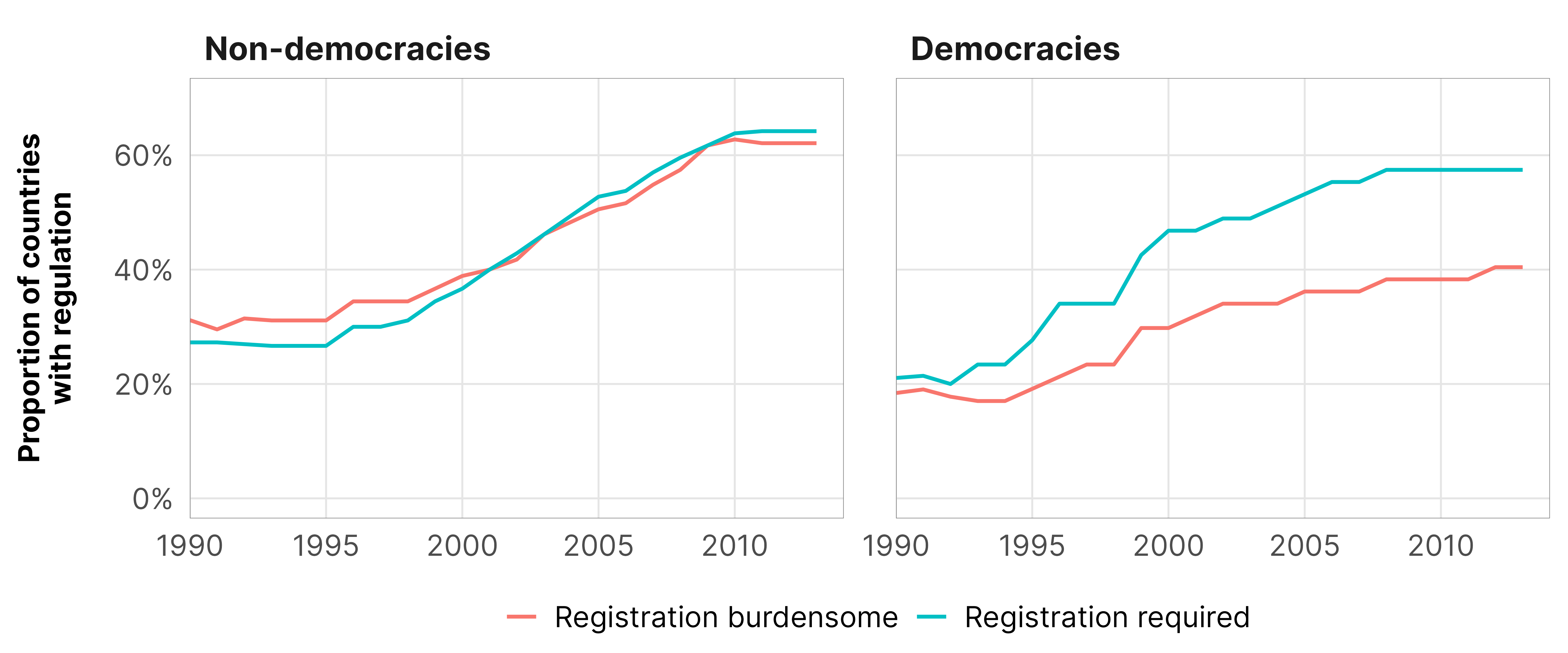
Laws requiring NGO registration aren’t necessarily a sign of oppression—even the US requires that nonprofits that earn above a certain threshold register as 501(c)(3) organizations. Though the figure below shows that compulsory regulation have increased over time, actual restriction has occurred too. Burdensome registration is not just another standard layer of bureaucracy.
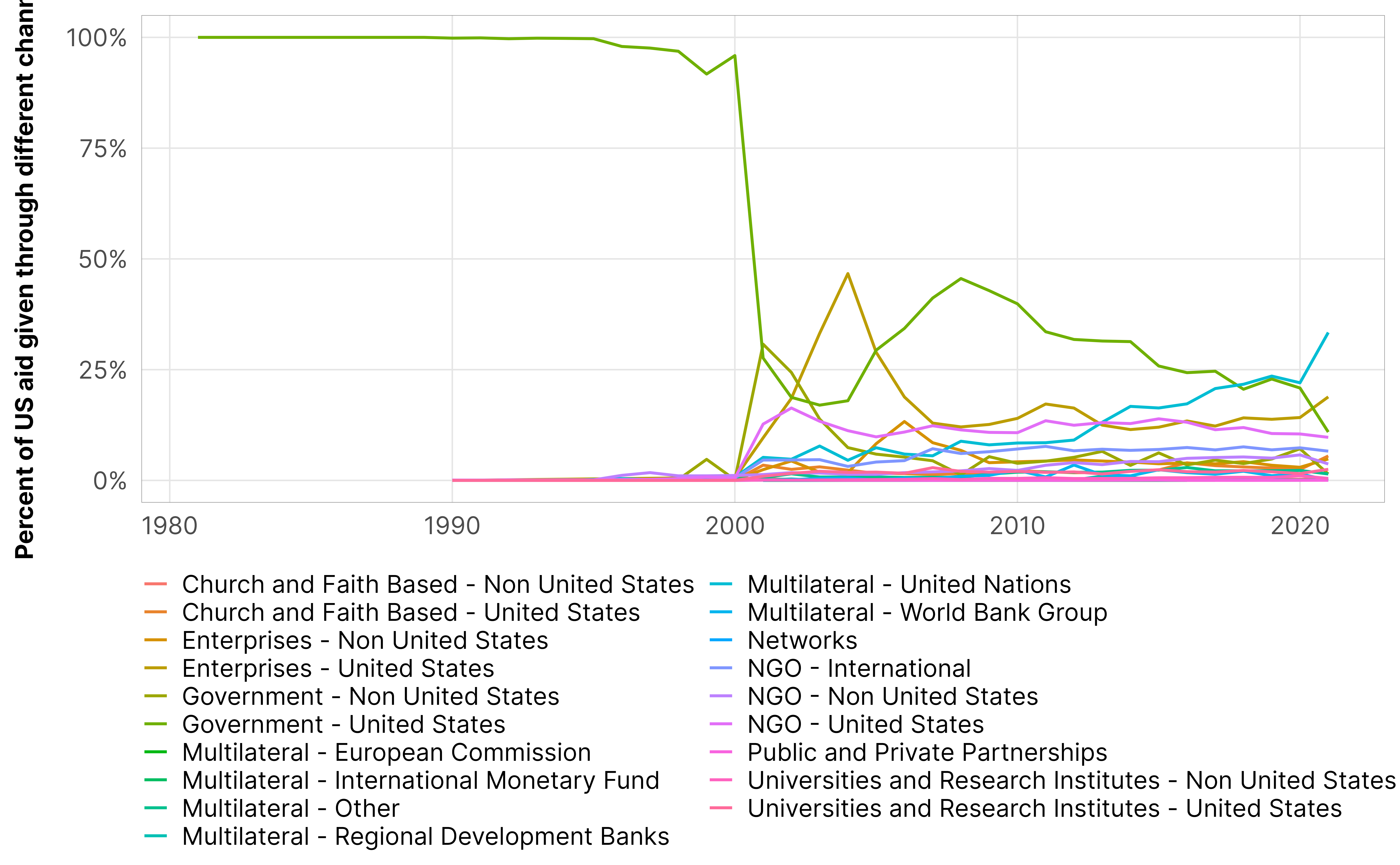
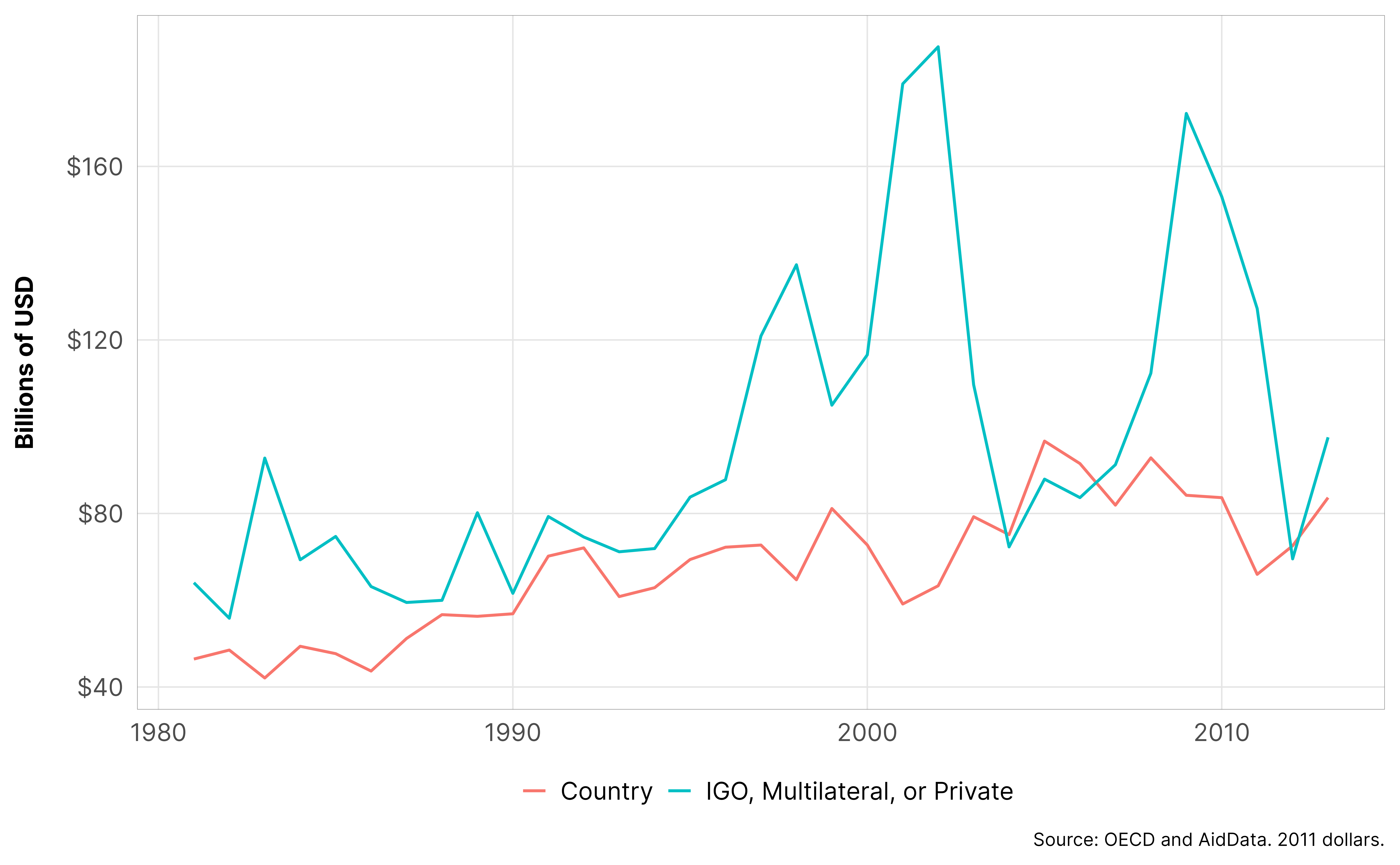
aid_donor_type_time <- df_donor %>%group_by(year, donor_type_collapsed) %>%summarise(total_aid =sum(oda, na.rm =TRUE))ggplot(aid_donor_type_time, aes(x = year, y = total_aid /1000000000,colour = donor_type_collapsed)) +geom_line(size =0.5) +labs(x =NULL, y ="Billions of USD",caption ="Source: OECD and AidData. 2011 dollars.") +guides(colour =guide_legend(title =NULL)) +scale_y_continuous(labels = dollar) +theme_donors()
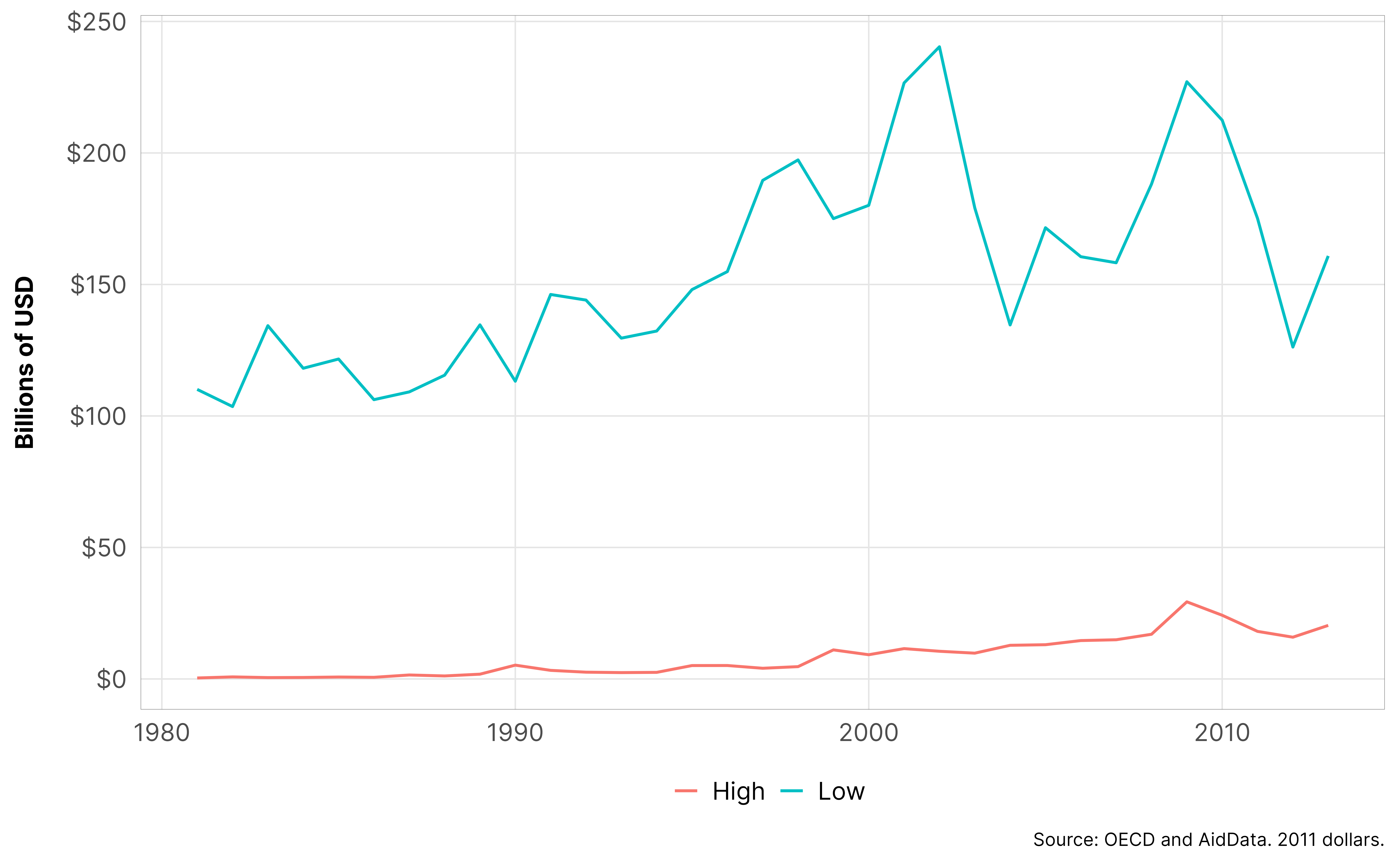
Aid over time, by contentiousness
Code
aid_contention_time <- df_donor %>%group_by(year, purpose_contentiousness) %>%summarise(total_aid =sum(oda, na.rm =TRUE))ggplot(aid_contention_time, aes(x = year, y = total_aid /1000000000,colour = purpose_contentiousness)) +geom_line(size =0.5) +labs(x =NULL, y ="Billions of USD",caption ="Source: OECD and AidData. 2011 dollars.") +guides(colour =guide_legend(title =NULL)) +scale_y_continuous(labels = dollar) +theme_donors()
Restrictions and aid
Code
inv_logit <-function(f, a) { a <- (1-2* a) (a * (1+exp(f)) + (exp(f) -1)) / (2* a * (1+exp(f)))}dvs_clean_names <-tribble(~barrier, ~barrier_clean,"barriers_total", "All barriers","advocacy", "Barriers to advocacy","entry", "Barriers to entry","funding", "Barriers to funding")ivs_clean_names <-tribble(~variable, ~variable_clean, ~hypothesis,"total_oda_lead1", "Total ODA", "H1","prop_contentious_lead1", "Contentious aid", "H2","prop_ngo_dom_lead1", "Aid to domestic NGOs", "H3","prop_ngo_foreign_lead1", "Aid to foreign NGOs", "H3")
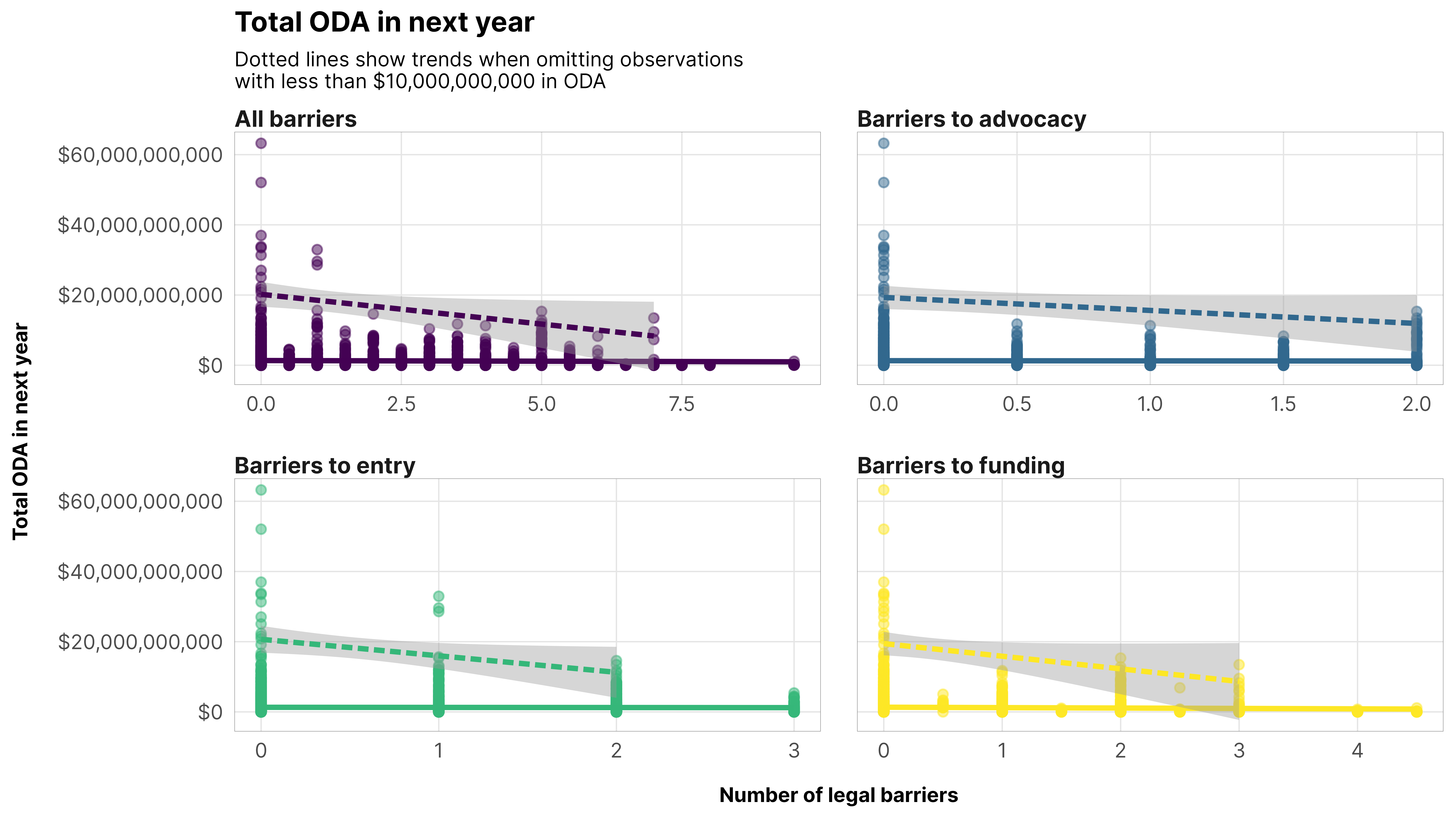
Restrictions and ODA (H1)
Code
df_plot_barriers_oda <- df_country_aid_laws %>%select(year, gwcode, country, total_oda_lead1,one_of(dvs_clean_names$barrier)) %>%pivot_longer(names_to ="barrier", values_to ="value", one_of(dvs_clean_names$barrier)) %>%left_join(dvs_clean_names, by ="barrier") %>%mutate(barrier_clean =fct_inorder(barrier_clean, ordered =TRUE))ggplot(df_plot_barriers_oda, aes(x = value, y = total_oda_lead1, color = barrier_clean)) +geom_point(alpha =0.5) +stat_smooth(method ="lm") +stat_smooth(data =filter(df_plot_barriers_oda, total_oda_lead1 >10000000000), method ="lm", linetype ="21") +scale_y_continuous(labels = dollar) +guides(color ="none") +labs(x ="Number of legal barriers", y ="Total ODA in next year",title ="Total ODA in next year",subtitle ="Dotted lines show trends when omitting observations\nwith less than $10,000,000,000 in ODA") +theme_donors(10) +theme(strip.text.x =element_text(margin =margin(t =1, b =1))) +facet_wrap(vars(barrier_clean), scales ="free_x", nrow =2)
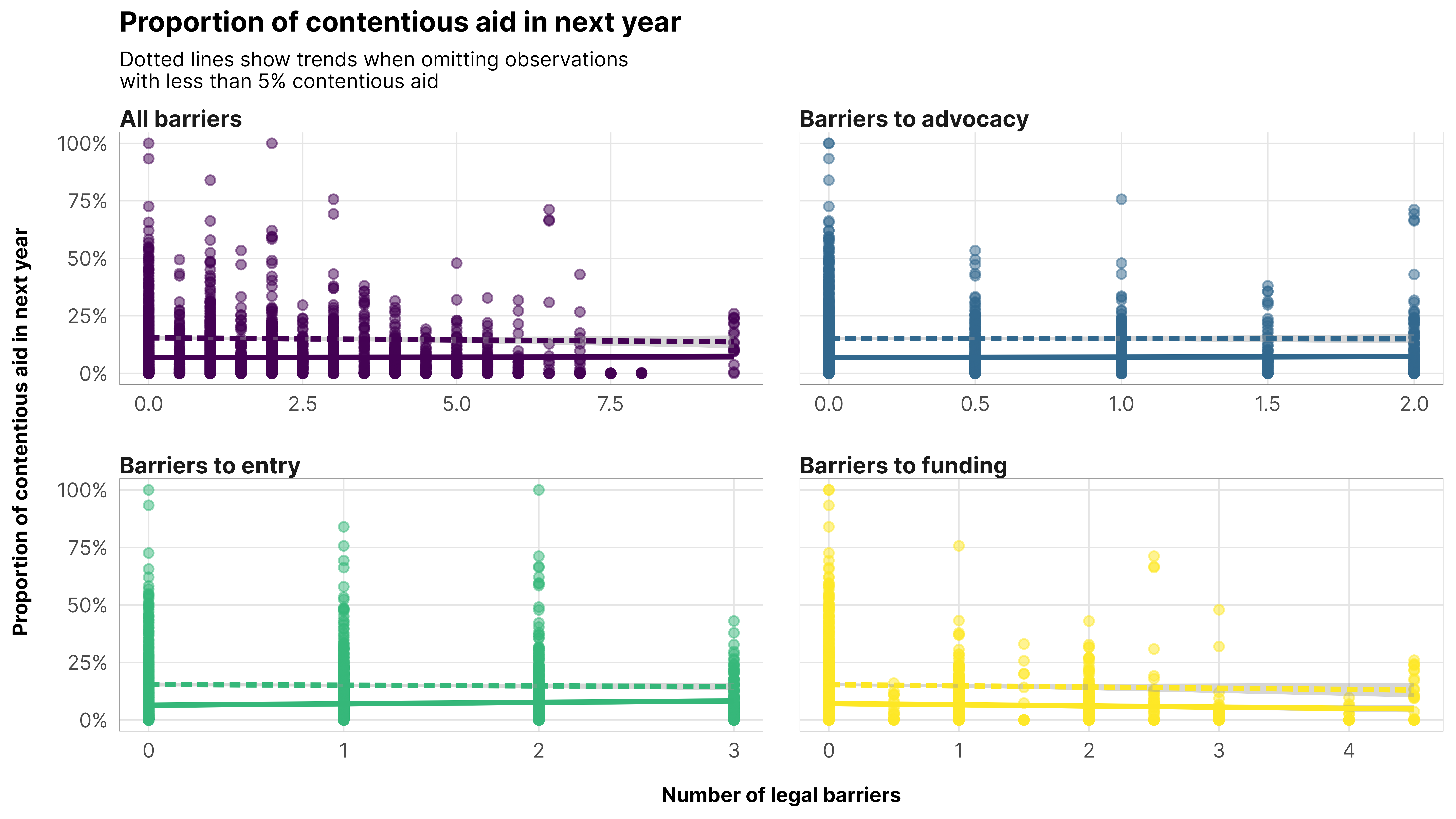
Restrictions and contentiousness (H2)
Code
df_plot_barriers_contention <- df_country_aid_laws %>%select(year, gwcode, country, prop_contentious_lead1,one_of(dvs_clean_names$barrier)) %>%pivot_longer(names_to ="barrier", values_to ="value", one_of(dvs_clean_names$barrier)) %>%left_join(dvs_clean_names, by ="barrier") %>%mutate(barrier_clean =fct_inorder(barrier_clean, ordered =TRUE))ggplot(df_plot_barriers_contention, aes(x = value, y = prop_contentious_lead1, color = barrier_clean)) +geom_point(alpha =0.5) +stat_smooth(method ="lm") +stat_smooth(data =filter(df_plot_barriers_contention, prop_contentious_lead1 >0.05), method ="lm", linetype ="21") +scale_y_continuous(labels = percent) +guides(color ="none") +labs(x ="Number of legal barriers", y ="Proportion of contentious aid in next year",title ="Proportion of contentious aid in next year",subtitle ="Dotted lines show trends when omitting observations\nwith less than 5% contentious aid") +theme_donors(10) +theme(strip.text.x =element_text(margin =margin(t =1, b =1))) +facet_wrap(vars(barrier_clean), scales ="free_x", nrow =2)
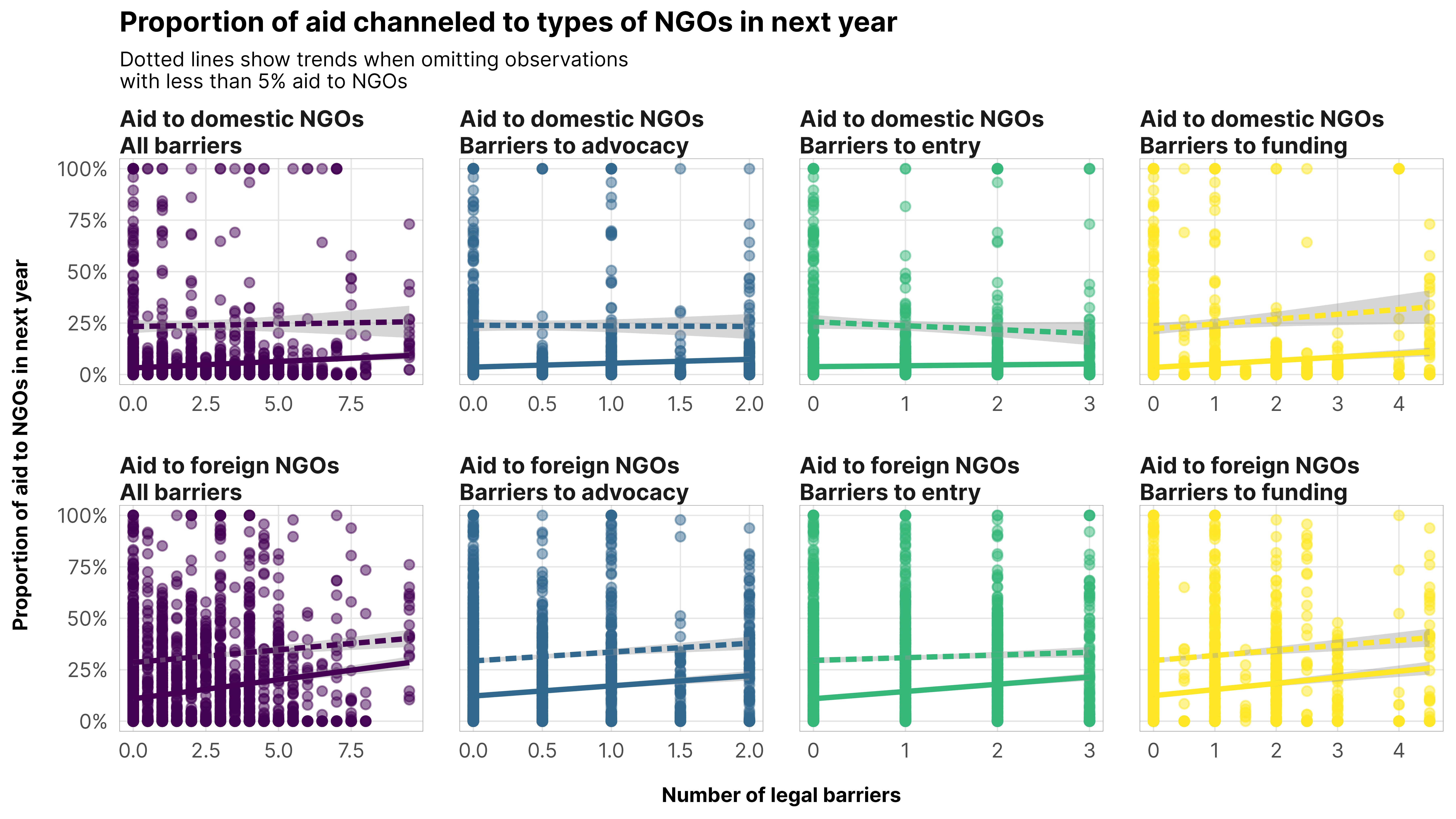
Restrictions and NGOs (H3)
Code
df_plot_barriers_ngos <- df_country_aid_laws %>%select(year, gwcode, country, prop_ngo_dom_lead1, prop_ngo_foreign_lead1,one_of(dvs_clean_names$barrier)) %>%pivot_longer(names_to ="barrier", values_to ="value", one_of(dvs_clean_names$barrier)) %>%pivot_longer(names_to ="ngo_type", values_to ="prop_ngo", c(prop_ngo_dom_lead1, prop_ngo_foreign_lead1)) %>%left_join(dvs_clean_names, by ="barrier") %>%left_join(ivs_clean_names, by =c("ngo_type"="variable")) %>%mutate(barrier_clean =fct_inorder(barrier_clean, ordered =TRUE))ggplot(df_plot_barriers_ngos, aes(x = value, y = prop_ngo, color = barrier_clean)) +geom_point(alpha =0.5) +stat_smooth(method ="lm") +stat_smooth(data =filter(df_plot_barriers_ngos, prop_ngo >0.05), method ="lm", linetype ="21") +scale_y_continuous(labels = percent) +guides(color ="none") +labs(x ="Number of legal barriers", y ="Proportion of aid to NGOs in next year",title ="Proportion of aid channeled to types of NGOs in next year",subtitle ="Dotted lines show trends when omitting observations\nwith less than 5% aid to NGOs") +coord_cartesian(ylim =c(0, 1)) +theme_donors(10) +theme(strip.text.x =element_text(margin =margin(t =1, b =1))) +facet_wrap(vars(variable_clean, barrier_clean), scales ="free_x", ncol =4)
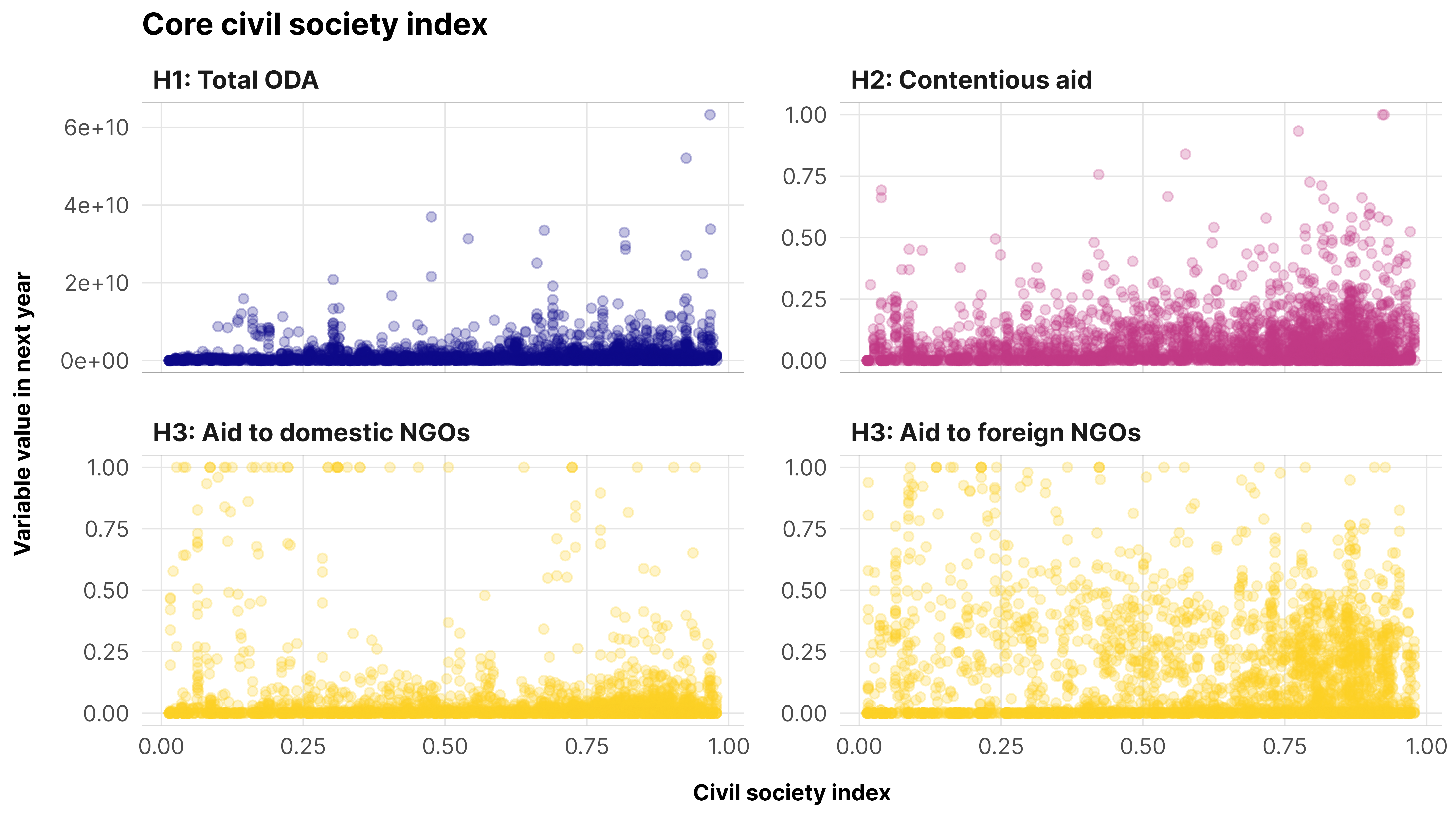
CCSI and all DVs (all hypotheses)
Code
df_plot_ccsi_ngos <- df_country_aid_laws %>%select(year, gwcode, country, one_of(ivs_clean_names$variable), v2xcs_ccsi) %>%pivot_longer(names_to ="variable", values_to ="value", c(one_of(ivs_clean_names$variable))) %>%left_join(ivs_clean_names, by ="variable") %>%mutate(hypothesis_clean =paste0(hypothesis, ": ", variable_clean)) %>%arrange(hypothesis_clean) %>%mutate(hypothesis_clean =fct_inorder(hypothesis_clean, ordered =TRUE))ggplot(df_plot_ccsi_ngos, aes(x = v2xcs_ccsi, y = value, color = hypothesis)) +geom_point(alpha =0.25) +scale_color_viridis_d(option ="plasma", end =0.9) +guides(color ="none") +labs(x ="Civil society index", y ="Variable value in next year",title ="Core civil society index") +theme_donors() +facet_wrap(vars(hypothesis_clean), scales ="free_y")
Coppedge, Michael, John Gerring, Carl Henrik Knutsen, Staffan I. Lindberg, Jan Teorell, David Altman, Michael Bernhard, et al. 2020. “V-Dem [Country-Year/Country-Date] Dataset V10.” Varieties of Democracy (V-Dem) Project. https://doi.org/10.23696/vdemds20.
Source Code
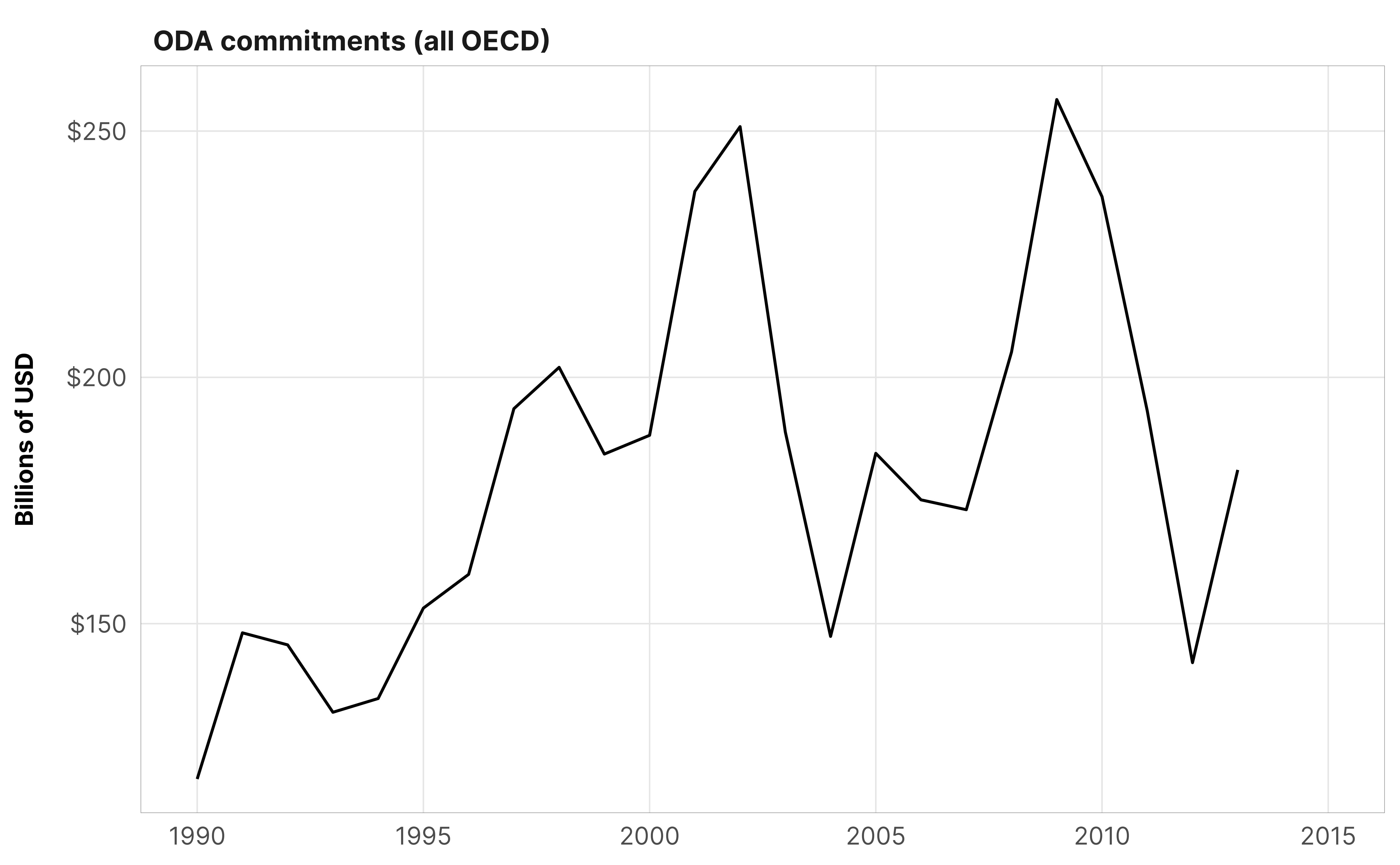
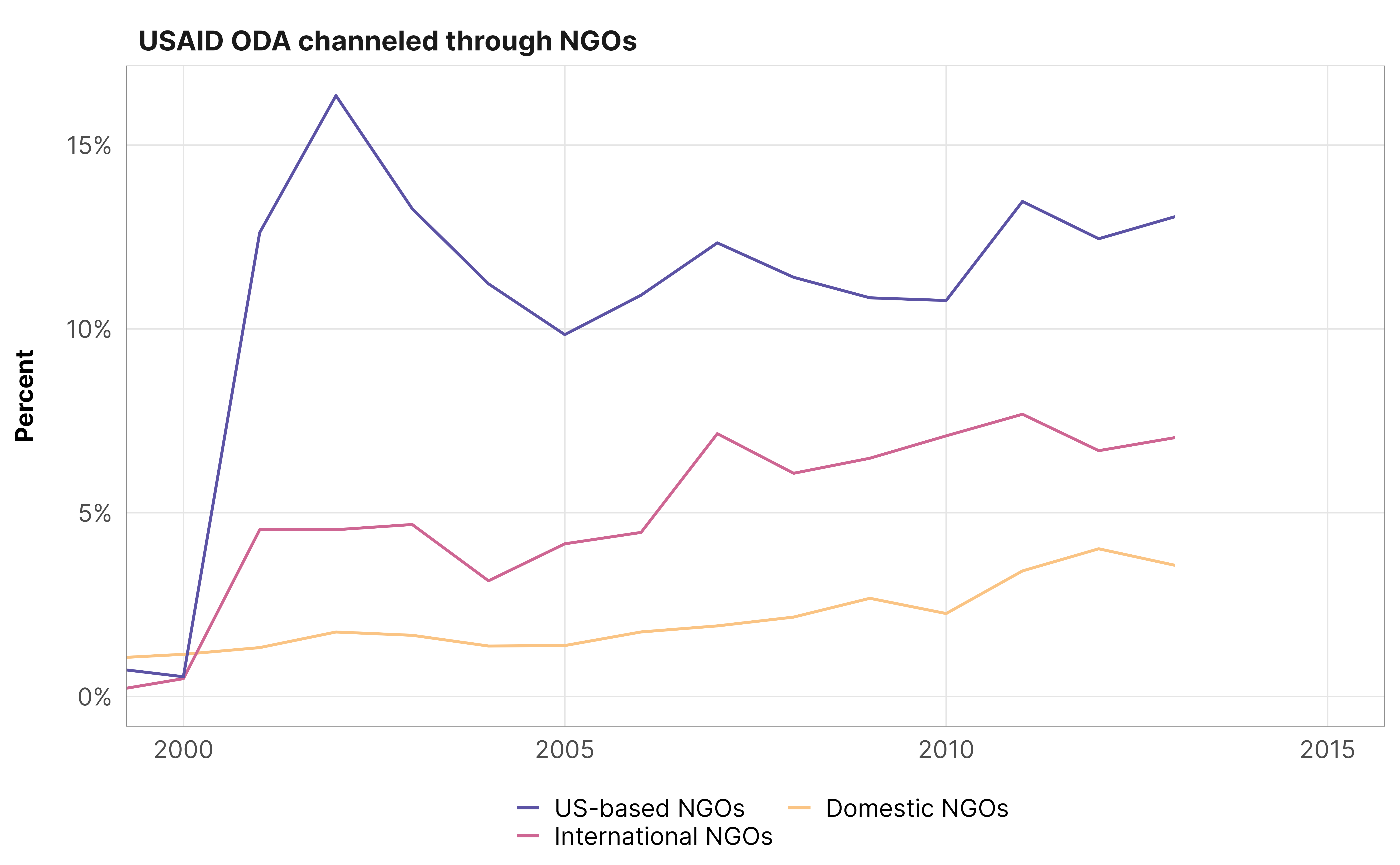
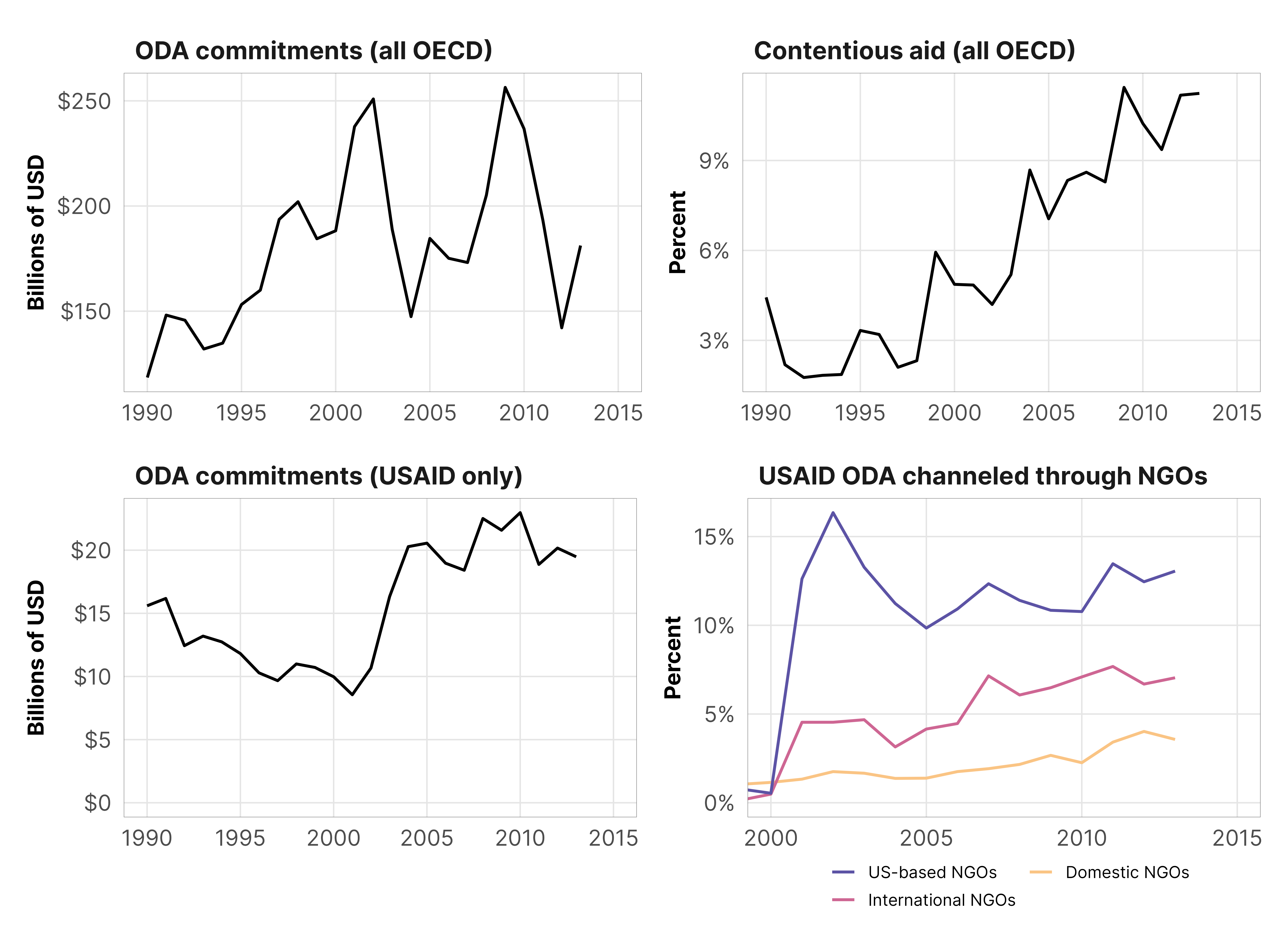
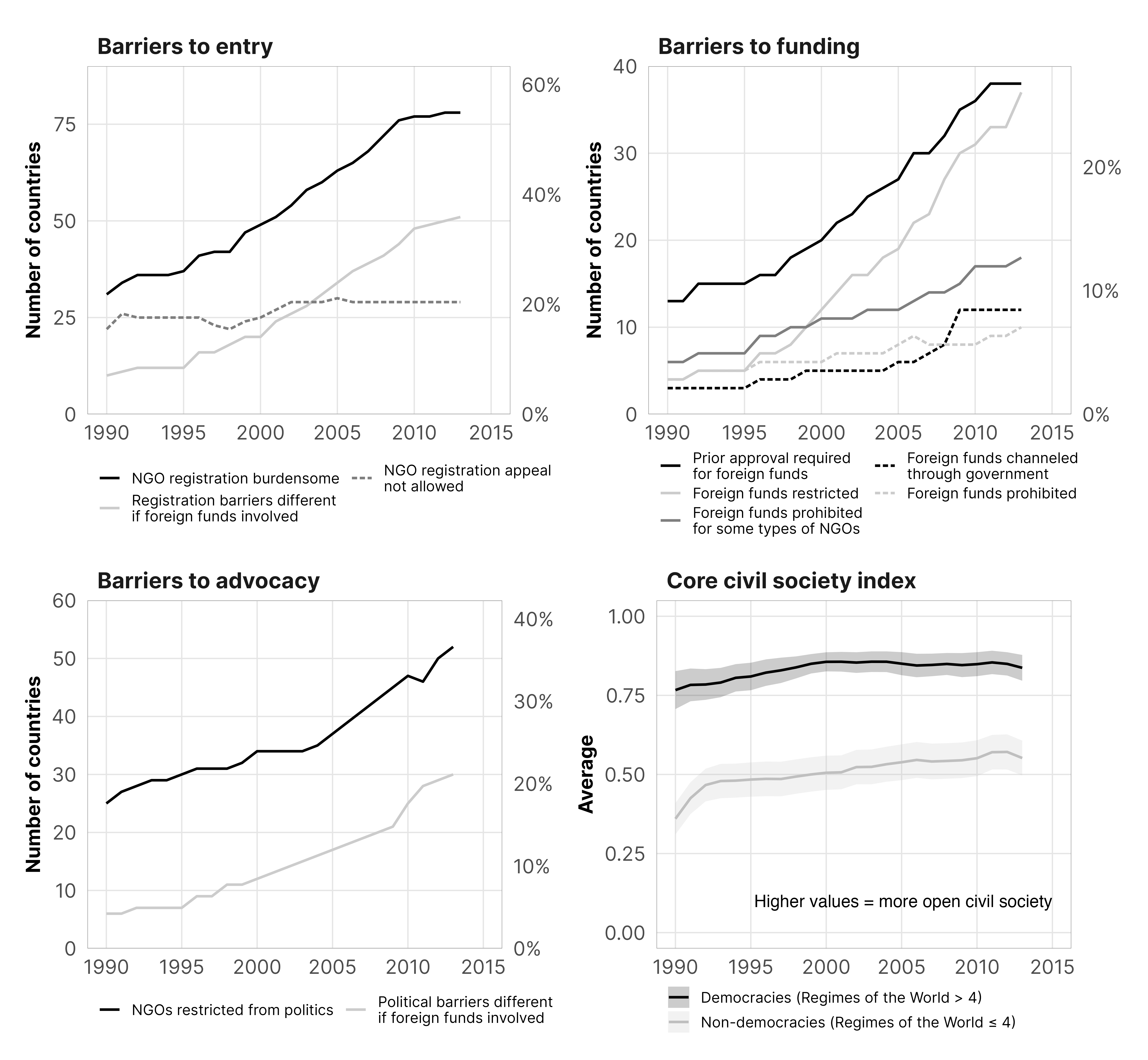
---title: "General analysis"author: "Suparna Chaudhry and Andrew Heiss"date: "`r format(Sys.time(), '%F')`"link-citations: trueeditor_options: chunk_output_type: console---```{r setup, include=FALSE}knitr::opts_chunk$set(fig.retina =3,tidy.opts =list(width.cutoff =120), # For codeoptions(width =90), # For outputfig.asp =0.618, fig.width =7, fig.align ="center", out.width ="85%")options(dplyr.summarise.inform =FALSE,knitr.kable.NA ="")``````{r load-libraries, warning=FALSE, message=FALSE}library(tidyverse)library(targets)library(scales)library(patchwork)library(kableExtra)library(sf)library(here)tar_config_set(store = here::here('_targets'),script = here::here('_targets.R'))# Load things from targetsinvisible(list2env(tar_read(graphic_functions), .GlobalEnv))invisible(list2env(tar_read(misc_funs), .GlobalEnv))df_donor <-tar_read(donor_level_data)df_donor_us <-tar_read(donor_level_data_usaid)df_country_aid <-tar_read(country_aid_final)df_country_aid_laws <-filter(df_country_aid, laws)df_autocracies <-tar_read(autocracies)vars_to_summarize <-tar_read(var_details) %>%mutate(summary_order =1:n())tar_load(c(ngo_index_table, regulations))tar_load(c(civicus_map_data, civicus_clean))my_seed <-1234set.seed(my_seed)```# Overall data summary```{r data-summary}num_countries <- df_country_aid_laws %>%distinct(gwcode) %>%nrow()num_years <- df_country_aid_laws %>%distinct(year) %>%nrow()year_first <- df_country_aid_laws %>%distinct(year) %>%min()year_last <- df_country_aid_laws %>%distinct(year) %>%max()```Our data includes information about `r num_countries` countries across `r num_years` years (from `r year_first`–`r year_last`)# Summary of variables in model(*From our AJPS submission*): The values here are slightly different from what we had at ISA and MPSA (and our ISQ submission) because we're now using V-Dem 8.0 and AidData 3.1. And now the values are even different-er, since we're using V-Dem 10.0 and have really clean data now.```{r summary-vars-model, message=FALSE, results="asis"}vars_summarized <- df_country_aid_laws %>%select(one_of(vars_to_summarize$term)) %>%mutate(total_oda = total_oda /1000000) %>%mutate(gdpcap_log =exp(gdpcap_log)) %>%pivot_longer(names_to ="term", values_to ="value", everything()) %>%filter(!is.na(value)) %>%group_by(term) %>%summarize(N =n(),Mean =mean(value),Median =median(value),`Std. Dev.`=sd(value),Min =min(value),Max =max(value)) %>%ungroup() %>%left_join(vars_to_summarize, by ="term") %>%arrange(summary_order) %>%mutate(across(c(Mean, `Std. Dev.`, Median, Min, Max),~case_when( format =="percent"~percent_format(accuracy =0.1)(.), format =="dollar"~dollar_format(accuracy =1)(.), format =="number"~comma_format(accuracy =0.1)(.)))) %>%mutate(N =comma(N)) %>%select(category, subcategory, Variable = term_clean_table, Source = source, Mean, `Std. Dev.`, Median, Min, Max, N)vars_summarized %>%select(-category, ``= subcategory) %>%kbl() %>%kable_styling() %>%pack_rows(index =table(fct_inorder(vars_summarized$category))) %>%collapse_rows(columns =1, valign ="top") %>%unclass() %>%cat()```# Aid stuff## Overall OECD aid```{r summarize-oecd-aid}total_oecd_aid <- df_country_aid_laws %>%summarise(total =dollar(sum(total_oda))) %>%pull(total)```OECD members donated `r total_oecd_aid` between 1990 and 2013.```{r plot-oecd-aid}plot_aid <- df_country_aid_laws %>%filter(year <=2013) %>%group_by(year) %>%summarise(total =sum(total_oda)) %>%mutate(fake_facet_title ="ODA commitments (all OECD)")fig_oecd_aid <-ggplot(plot_aid, aes(x = year, y = (total /1000000000))) +geom_line(size =0.5) +labs(x =NULL, y ="Billions of USD") +scale_y_continuous(labels = dollar) +coord_cartesian(xlim =c(1990, 2015)) +theme_donors() +facet_wrap(vars(fake_facet_title))fig_oecd_aid```## Proportion of contentious vs. noncontentious aid```{r summarize-contentious-aid}df_donor %>%filter(year >=1990) %>%group_by(purpose_contentiousness) %>%summarise(Total =sum(oda)) %>%ungroup() %>%mutate(Percent = Total /sum(Total)) %>%mutate(Total =dollar(Total), Percent =percent_format(accuracy =0.1)(Percent)) %>%rename(`Contentiousness`= purpose_contentiousness) %>%kbl() %>%kable_styling(full_width =FALSE)``````{r plot-contentious-aid}plot_aid_contentiousness <- df_donor %>%filter(year >=1990) %>%group_by(year, purpose_contentiousness) %>%summarise(total =sum(oda)) %>%mutate(perc = total /sum(total)) %>%filter(purpose_contentiousness =="High") %>%mutate(fake_facet_title ="Contentious aid (all OECD)")fig_oecd_contention <-ggplot(plot_aid_contentiousness, aes(x = year, y = perc)) +geom_line(size =0.5) +scale_y_continuous(labels =percent_format(accuracy =1)) +labs(x =NULL, y ="Percent") +coord_cartesian(xlim =c(1990, 2015)) +theme_donors() +facet_wrap(vars(fake_facet_title))fig_oecd_contention```## USAID aid```{r summarize-us-aid}total_us_aid <- df_country_aid_laws %>%summarise(total =dollar(sum(oda_us))) %>%pull(total)total_us_aid_post_2000 <- df_country_aid_laws %>%filter(year >1999) %>%summarise(total =dollar(sum(oda_us))) %>%pull(total)```The US donated `r total_us_aid` between 1990 and 2014 and `r total_us_aid_post_2000` between 2000 and 2014.```{r plot-us-aid}plot_aid_us <- df_country_aid_laws %>%filter(year >=1990) %>%group_by(year) %>%summarise(total =sum(oda_us)) %>%mutate(fake_facet_title ="ODA commitments (USAID only)")fig_us_aid <-ggplot(plot_aid_us, aes(x = year, y = (total /1000000000))) +geom_line(size =0.5) +expand_limits(y =0) +labs(x =NULL, y ="Billions of USD") +scale_y_continuous(labels = dollar) +coord_cartesian(xlim =c(1990, 2015)) +theme_donors() +facet_wrap(vars(fake_facet_title))fig_us_aid```## Proportion of US aid to types of NGOsTotal amounts over time:```{r summarize-aid-channels}usaid_total <- df_country_aid_laws %>%summarise(total =sum(oda_us)) %>%pull(total)channels_nice <-tribble(~channel, ~channel_clean,"oda_us_ngo_dom", "Domestic NGOs","oda_us_ngo_int", "International NGOs","oda_us_ngo_us", "US-based NGOs")df_country_aid_laws %>%pivot_longer(names_to ="channel", values_to ="total_oda_us",c(oda_us_ngo_dom, oda_us_ngo_int, oda_us_ngo_us)) %>%group_by(channel) %>%summarise(total =sum(total_oda_us)) %>%ungroup() %>%left_join(channels_nice, by ="channel") %>%mutate(perc = total / usaid_total) %>%mutate(total =dollar(total), perc =percent(perc)) %>%select(Channel = channel_clean, Total = total, Percent = perc) %>%kbl() %>%kable_styling(full_width =FALSE)```The US clearly favors US-based NGOs or international NGOs over domestic NGOs.```{r plot-aid-channels}usaid_total_yearly <- df_country_aid_laws %>%group_by(year) %>%summarise(annual_total =sum(oda_us)) %>%mutate(fake_facet_title ="USAID ODA channeled through NGOs")plot_usaid_channel <- df_country_aid_laws %>%filter(year >=1990) %>%pivot_longer(names_to ="channel", values_to ="total_oda_us", c(oda_us_ngo_dom, oda_us_ngo_int, oda_us_ngo_us)) %>%group_by(year, channel) %>%summarise(total =sum(total_oda_us)) %>%left_join(usaid_total_yearly, by ="year") %>%mutate(perc = total / annual_total) %>%left_join(channels_nice, by ="channel")fig_usaid_channel <-ggplot(plot_usaid_channel, aes(x = year, y = perc, colour = channel_clean)) +geom_line(size =0.5) +scale_y_continuous(labels =percent_format(accuracy =1)) +scale_colour_manual(values = clrs$Sunset[c(2, 5, 7)]) +labs(x =NULL, y ="Percent") +guides(colour =guide_legend(title =NULL, reverse =TRUE, nrow =2)) +coord_cartesian(xlim =c(1990, 2015)) +theme_donors() +facet_wrap(vars(fake_facet_title))fig_usaid_channel```USAID data categorizes all aid as government-channeled before 2000 because of some quirk in the data.```{r plot-all-channels}plot_usaid_channels_all <- df_donor_us %>%group_by(year, implementing_partner_sub_category_name) %>%summarise(total =sum(oda_us_2011)) %>%mutate(perc = total /sum(total)) %>%mutate(channel =ifelse(str_detect(implementing_partner_sub_category_name, "NGO"), "NGO", "Other"))ggplot(plot_usaid_channels_all, aes(x = year, y = perc, colour = implementing_partner_sub_category_name)) +geom_line(size =0.5) +scale_y_continuous(labels =percent_format(accuracy =1)) +labs(x =NULL, y ="Percent of US aid given through different channels") +guides(colour =guide_legend(title =NULL, ncol =2)) +theme_donors()```So we just look at aid after 2000.```{r plot-channels-post-2000, warning=FALSE, message=FALSE}fig_usaid_channel_trimmed <- fig_usaid_channel +coord_cartesian(xlim =c(2000, 2015))fig_usaid_channel_trimmed```## All DV figures combined```{r plot-all-dvs, fig.width=6.5, fig.height=4.75, fig.asp=NULL}fig_dvs <- (fig_oecd_aid + fig_oecd_contention) / (fig_us_aid + fig_usaid_channel_trimmed) &theme_donors(base_size =10) +theme(legend.text =element_text(size =rel(0.6)),axis.title.y =element_text(margin =margin(r =3)),legend.box.margin =margin(t =-0.5, unit ="lines"))fig_dvs# ggsave(here("analysis", "output", "fig-dvs.pdf"), fig_dvs,# width = 6.5, height = 4.75, device = cairo_pdf)# ggsave(here("analysis", "output", "fig-dvs.png"), fig_dvs,# width = 6.5, height = 4.75, res = 300, device = ragg::agg_png)```# Legal restrictions on NGOs## DCJW / Chaudhry indexes```{r dcjw-index-table}ngo_index_table <- ngo_index_table %>%mutate(Index_nice =paste0(Index, " (max: ", Max, ")"))ngo_index_table %>%select(`Restriction description`= Description, Coding) %>%kbl(align =c("l", "l"),caption ="Description of indexes of NGO barriers") %>%kable_styling() %>%pack_rows(index =table(fct_inorder(ngo_index_table$Index_nice)),indent =FALSE)```## NGO barriers over time```{r advocacy-laws, message=FALSE, fig.width=6.5, fig.height=6, fig.asp=NULL}regulations <- regulations %>%filter(!ignore_in_index) %>%mutate(barrier_group =paste0("Barriers to ", str_to_lower(barrier))) %>%select(barrier_group, barrier = question_clean, barrier_display = question_display)df_barriers <- df_country_aid_laws %>%group_by(gwcode, year) %>%summarize(across(one_of(regulations$barrier), ~. >0)) %>%group_by(year) %>%summarize(across(-gwcode, ~sum(.))) %>%ungroup() %>%pivot_longer(names_to ="barrier", values_to ="value", -year) %>%left_join(regulations, by ="barrier") %>%mutate(barrier_display =str_replace(barrier_display, "XXX", "\n")) %>%arrange(desc(value)) %>%mutate(barrier_display =fct_inorder(barrier_display, ordered =TRUE))dcjw_entry_plot <-ggplot(filter(df_barriers, barrier_group =="Barriers to entry"), aes(x = year, y = value, color = barrier_display,linetype = barrier_display)) +geom_line(size =0.5) +expand_limits(y =c(0, 90)) +scale_y_continuous(sec.axis =sec_axis(~ . / num_countries,labels =percent_format(accuracy =1)),expand =c(0, 0)) +scale_colour_manual(values =c("black", "grey80", "grey50"), name =NULL) +scale_linetype_manual(values =c("solid", "solid", "21"), name =NULL) +coord_cartesian(xlim =c(1990, 2015), ylim =c(0, 90)) +guides(color =guide_legend(nrow =2)) +labs(x =NULL, y ="Number of countries") +theme_donors(10) +theme(legend.justification ="left") +facet_wrap(vars(barrier_group))dcjw_funding_plot <-ggplot(filter(df_barriers, barrier_group =="Barriers to funding"), aes(x = year, y = value, color = barrier_display,linetype = barrier_display)) +geom_line(size =0.5) +scale_y_continuous(sec.axis =sec_axis(~ . / num_countries,labels =percent_format(accuracy =1)),expand =c(0, 0)) +scale_colour_manual(values =c("black", "grey80", "grey50", "black", "grey80"), name =NULL) +scale_linetype_manual(values =c("solid", "solid", "solid", "21", "21"), name =NULL) +coord_cartesian(xlim =c(1990, 2015), ylim =c(0, 40)) +guides(color =guide_legend(nrow =3),linetype =guide_legend(nrow =3)) +labs(x =NULL, y ="Number of countries") +theme_donors(10) +theme(legend.justification ="left") +facet_wrap(vars(barrier_group))dcjw_advocacy_plot <-ggplot(filter(df_barriers, barrier_group =="Barriers to advocacy"), aes(x = year, y = value, color = barrier_display)) +geom_line(size =0.5) +scale_y_continuous(sec.axis =sec_axis(~ . / num_countries,labels =percent_format(accuracy =1)),expand =c(0, 0)) +scale_colour_manual(values =c("black", "grey80"), name =NULL) +coord_cartesian(xlim =c(1990, 2015), ylim =c(0, 60)) +guides(color =guide_legend(nrow =1)) +labs(x =NULL, y ="Number of countries") +theme_donors(10) +theme(legend.justification ="left") +facet_wrap(vars(barrier_group))df_ccsi_plot <- df_country_aid %>%left_join(df_autocracies, by ="gwcode") %>%group_by(year, autocracy) %>%nest() %>%mutate(cis = data %>%map(~mean_cl_normal(.$v2xcs_ccsi))) %>%unnest(cis) %>%ungroup() %>%mutate(fake_facet_title ="Core civil society index",autocracy =factor(autocracy, labels =c("Democracies (Regimes of the World > 4)","Non-democracies (Regimes of the World ≤ 4)"), ordered =TRUE))fig_ccsi <-ggplot(df_ccsi_plot, aes(x = year, y = y)) +geom_ribbon(aes(ymin = ymin, ymax = ymax, fill = autocracy), alpha =0.2) +geom_line(aes(color = autocracy), size =0.5) +annotate(geom ="text", x =2015, y =0.1, hjust ="right", size =pts(7),label ="Higher values = more open civil society") +scale_colour_manual(values =c("black", "grey75"), name =NULL) +scale_fill_manual(values =c("black", "grey75"), name =NULL) +scale_linetype_manual(values =c("solid", "solid", "21")) +coord_cartesian(xlim =c(1990, 2015), ylim =c(0, 1)) +guides(color =guide_legend(nrow =2)) +labs(y ="Average", x =NULL) +theme_donors(10) +theme(legend.justification ="left") +facet_wrap(vars(fake_facet_title))barriers_summary <- ((dcjw_entry_plot + dcjw_funding_plot) / (dcjw_advocacy_plot + fig_ccsi)) &theme(legend.text =element_text(size =rel(0.6)),axis.title.y =element_text(margin =margin(r =3)),legend.box.margin =margin(t =-0.5, unit ="lines"))barriers_summary# ggsave(here("analysis", "output", "fig-barriers-summary.pdf"), barriers_summary,# width = 6.5, height = 6, device = cairo_pdf)# ggsave(here("analysis", "output", "fig-barriers-summary.png"), barriers_summary,# width = 6.5, height = 6, res = 300, device = ragg::agg_png)```## Compulsory vs. burdensome registrationLaws requiring NGO registration aren't necessarily a sign of oppression—even the US requires that nonprofits that earn above a certain threshold register as 501(c)(3) organizations. Though the figure below shows that compulsory regulation have increased over time, actual restriction has occurred too. Burdensome registration is not just another standard layer of bureaucracy.```{r compulsory-vs-burdensome, fig.width=6, fig.height=2.5, fig.asp=NULL}df_regulation <- df_country_aid_laws %>%left_join(select(df_autocracies, gwcode, autocracy), by ="gwcode") %>%group_by(year, autocracy) %>%summarise(`Registration required`=sum(ngo_register) /n(),`Registration burdensome`=sum(ngo_register_burden) /n()) %>%ungroup() %>%pivot_longer(names_to ="type_of_law", values_to ="value", -c(year, autocracy)) %>%mutate(autocracy =factor(autocracy, levels =c(TRUE, FALSE),labels =c("Non-democracies", "Democracies")))fig_regulation_burden <-ggplot(df_regulation, aes(x = year, y = value, color = type_of_law)) +geom_line(size =0.5) +scale_y_continuous(labels =percent_format(accuracy =1)) +scale_x_continuous(expand =c(0, 0)) +coord_cartesian(ylim =c(0, 0.7), xlim =c(1990, 2014)) +guides(colour =guide_legend(title =NULL)) +labs(x =NULL, y ="Proportion of countries\nwith regulation") +theme_donors(10) +facet_wrap(vars(autocracy))fig_regulation_burden# ggsave(here("analysis", "output", "fig-regulation-burden.pdf"), fig_dvs,# width = 6, height = 2.5, device = cairo_pdf)# ggsave(here("analysis", "output", "fig-regulation-burden.png"), fig_dvs,# width = 6, height = 2.5, res = 300, device = ragg::agg_png)```# Aid## Aid over time, by donor type```{r aid-by-donor}aid_donor_type_time <- df_donor %>%group_by(year, donor_type_collapsed) %>%summarise(total_aid =sum(oda, na.rm =TRUE))ggplot(aid_donor_type_time, aes(x = year, y = total_aid /1000000000,colour = donor_type_collapsed)) +geom_line(size =0.5) +labs(x =NULL, y ="Billions of USD",caption ="Source: OECD and AidData. 2011 dollars.") +guides(colour =guide_legend(title =NULL)) +scale_y_continuous(labels = dollar) +theme_donors()```## Aid over time, by contentiousness```{r aid-by-contention}aid_contention_time <- df_donor %>%group_by(year, purpose_contentiousness) %>%summarise(total_aid =sum(oda, na.rm =TRUE))ggplot(aid_contention_time, aes(x = year, y = total_aid /1000000000,colour = purpose_contentiousness)) +geom_line(size =0.5) +labs(x =NULL, y ="Billions of USD",caption ="Source: OECD and AidData. 2011 dollars.") +guides(colour =guide_legend(title =NULL)) +scale_y_continuous(labels = dollar) +theme_donors()```# Restrictions and aid {.tabset .tabset-fade .tabset-pills}```{r restrictions-aid-correlations}inv_logit <-function(f, a) { a <- (1-2* a) (a * (1+exp(f)) + (exp(f) -1)) / (2* a * (1+exp(f)))}dvs_clean_names <-tribble(~barrier, ~barrier_clean,"barriers_total", "All barriers","advocacy", "Barriers to advocacy","entry", "Barriers to entry","funding", "Barriers to funding")ivs_clean_names <-tribble(~variable, ~variable_clean, ~hypothesis,"total_oda_lead1", "Total ODA", "H1","prop_contentious_lead1", "Contentious aid", "H2","prop_ngo_dom_lead1", "Aid to domestic NGOs", "H3","prop_ngo_foreign_lead1", "Aid to foreign NGOs", "H3")```## Restrictions and ODA (H~1~)```{r restrictions-aid-h1, warning=FALSE, message=FALSE, fig.width=8, fig.height=4.5, fig.asp=NULL}df_plot_barriers_oda <- df_country_aid_laws %>%select(year, gwcode, country, total_oda_lead1,one_of(dvs_clean_names$barrier)) %>%pivot_longer(names_to ="barrier", values_to ="value", one_of(dvs_clean_names$barrier)) %>%left_join(dvs_clean_names, by ="barrier") %>%mutate(barrier_clean =fct_inorder(barrier_clean, ordered =TRUE))ggplot(df_plot_barriers_oda, aes(x = value, y = total_oda_lead1, color = barrier_clean)) +geom_point(alpha =0.5) +stat_smooth(method ="lm") +stat_smooth(data =filter(df_plot_barriers_oda, total_oda_lead1 >10000000000), method ="lm", linetype ="21") +scale_y_continuous(labels = dollar) +guides(color ="none") +labs(x ="Number of legal barriers", y ="Total ODA in next year",title ="Total ODA in next year",subtitle ="Dotted lines show trends when omitting observations\nwith less than $10,000,000,000 in ODA") +theme_donors(10) +theme(strip.text.x =element_text(margin =margin(t =1, b =1))) +facet_wrap(vars(barrier_clean), scales ="free_x", nrow =2)```## Restrictions and contentiousness (H~2~)```{r restrictions-aid-h2, warning=FALSE, message=FALSE, fig.width=8, fig.height=4.5, fig.asp=NULL}df_plot_barriers_contention <- df_country_aid_laws %>%select(year, gwcode, country, prop_contentious_lead1,one_of(dvs_clean_names$barrier)) %>%pivot_longer(names_to ="barrier", values_to ="value", one_of(dvs_clean_names$barrier)) %>%left_join(dvs_clean_names, by ="barrier") %>%mutate(barrier_clean =fct_inorder(barrier_clean, ordered =TRUE))ggplot(df_plot_barriers_contention, aes(x = value, y = prop_contentious_lead1, color = barrier_clean)) +geom_point(alpha =0.5) +stat_smooth(method ="lm") +stat_smooth(data =filter(df_plot_barriers_contention, prop_contentious_lead1 >0.05), method ="lm", linetype ="21") +scale_y_continuous(labels = percent) +guides(color ="none") +labs(x ="Number of legal barriers", y ="Proportion of contentious aid in next year",title ="Proportion of contentious aid in next year",subtitle ="Dotted lines show trends when omitting observations\nwith less than 5% contentious aid") +theme_donors(10) +theme(strip.text.x =element_text(margin =margin(t =1, b =1))) +facet_wrap(vars(barrier_clean), scales ="free_x", nrow =2)```## Restrictions and NGOs (H~3~)```{r restrictions-aid-h3, warning=FALSE, message=FALSE, fig.width=8, fig.height=4.5, fig.asp=NULL}df_plot_barriers_ngos <- df_country_aid_laws %>%select(year, gwcode, country, prop_ngo_dom_lead1, prop_ngo_foreign_lead1,one_of(dvs_clean_names$barrier)) %>%pivot_longer(names_to ="barrier", values_to ="value", one_of(dvs_clean_names$barrier)) %>%pivot_longer(names_to ="ngo_type", values_to ="prop_ngo", c(prop_ngo_dom_lead1, prop_ngo_foreign_lead1)) %>%left_join(dvs_clean_names, by ="barrier") %>%left_join(ivs_clean_names, by =c("ngo_type"="variable")) %>%mutate(barrier_clean =fct_inorder(barrier_clean, ordered =TRUE))ggplot(df_plot_barriers_ngos, aes(x = value, y = prop_ngo, color = barrier_clean)) +geom_point(alpha =0.5) +stat_smooth(method ="lm") +stat_smooth(data =filter(df_plot_barriers_ngos, prop_ngo >0.05), method ="lm", linetype ="21") +scale_y_continuous(labels = percent) +guides(color ="none") +labs(x ="Number of legal barriers", y ="Proportion of aid to NGOs in next year",title ="Proportion of aid channeled to types of NGOs in next year",subtitle ="Dotted lines show trends when omitting observations\nwith less than 5% aid to NGOs") +coord_cartesian(ylim =c(0, 1)) +theme_donors(10) +theme(strip.text.x =element_text(margin =margin(t =1, b =1))) +facet_wrap(vars(variable_clean, barrier_clean), scales ="free_x", ncol =4)```## CCSI and all DVs (all hypotheses)```{r ccsi-aid-allhs, warning=FALSE, fig.width=8, fig.height=4.5, fig.asp=NULL}df_plot_ccsi_ngos <- df_country_aid_laws %>%select(year, gwcode, country, one_of(ivs_clean_names$variable), v2xcs_ccsi) %>%pivot_longer(names_to ="variable", values_to ="value", c(one_of(ivs_clean_names$variable))) %>%left_join(ivs_clean_names, by ="variable") %>%mutate(hypothesis_clean =paste0(hypothesis, ": ", variable_clean)) %>%arrange(hypothesis_clean) %>%mutate(hypothesis_clean =fct_inorder(hypothesis_clean, ordered =TRUE))ggplot(df_plot_ccsi_ngos, aes(x = v2xcs_ccsi, y = value, color = hypothesis)) +geom_point(alpha =0.25) +scale_color_viridis_d(option ="plasma", end =0.9) +guides(color ="none") +labs(x ="Civil society index", y ="Variable value in next year",title ="Core civil society index") +theme_donors() +facet_wrap(vars(hypothesis_clean), scales ="free_y")```# CIVICUS restrictions```{r civicus-numbers}civicus_clean %>%filter(!is.na(category)) %>%count(Rating = category, name ="Count") %>%arrange(desc(Rating)) %>%kbl(align =c("l", "c")) %>%kable_styling(full_width =FALSE)``````{r civicus-map, fig.width=5.5, fig.height=3, fig.asp=NULL}plot_civicus_map <-ggplot() +geom_sf(data = civicus_map_data, aes(fill =fct_rev(category)), size =0.15, color ="black") +coord_sf(crs =st_crs("ESRI:54030"), datum =NA) +# Robinson# scale_fill_manual(values = c("grey90", "grey70", "grey45",# "grey20", "black"),# na.translate = FALSE, name = "Civic space") +scale_fill_viridis_d(option ="plasma", end =0.9, na.translate =FALSE, name ="Civic space") +theme_donors_map() +theme(legend.position ="bottom",legend.key.size =unit(0.7, "lines"))plot_civicus_map# ggsave(here("analysis", "output", "fig-civicus-map.pdf"), plot_civicus_map,# width = 5.5, height = 3, device = cairo_pdf)# ggsave(here("analysis", "output", "fig-civicus-map-new.png"), plot_civicus_map,# width = 5.5, height = 3, res = 300, device = ragg::agg_png)```# List of countries included in models```{r list-countries, results="asis"}ncol_countries <-4all_countries <- df_country_aid_laws %>%distinct(country) %>%arrange(country) %>%pull(country) countries_caption <-paste0("All countries included in models (N = ", length(all_countries), ")")all_countries %>%matrix_from_vector(ncol = ncol_countries) %>%kbl(caption = countries_caption) %>%kable_styling(bootstrap_options =c("condensed", "striped"), full_width =FALSE)```# References