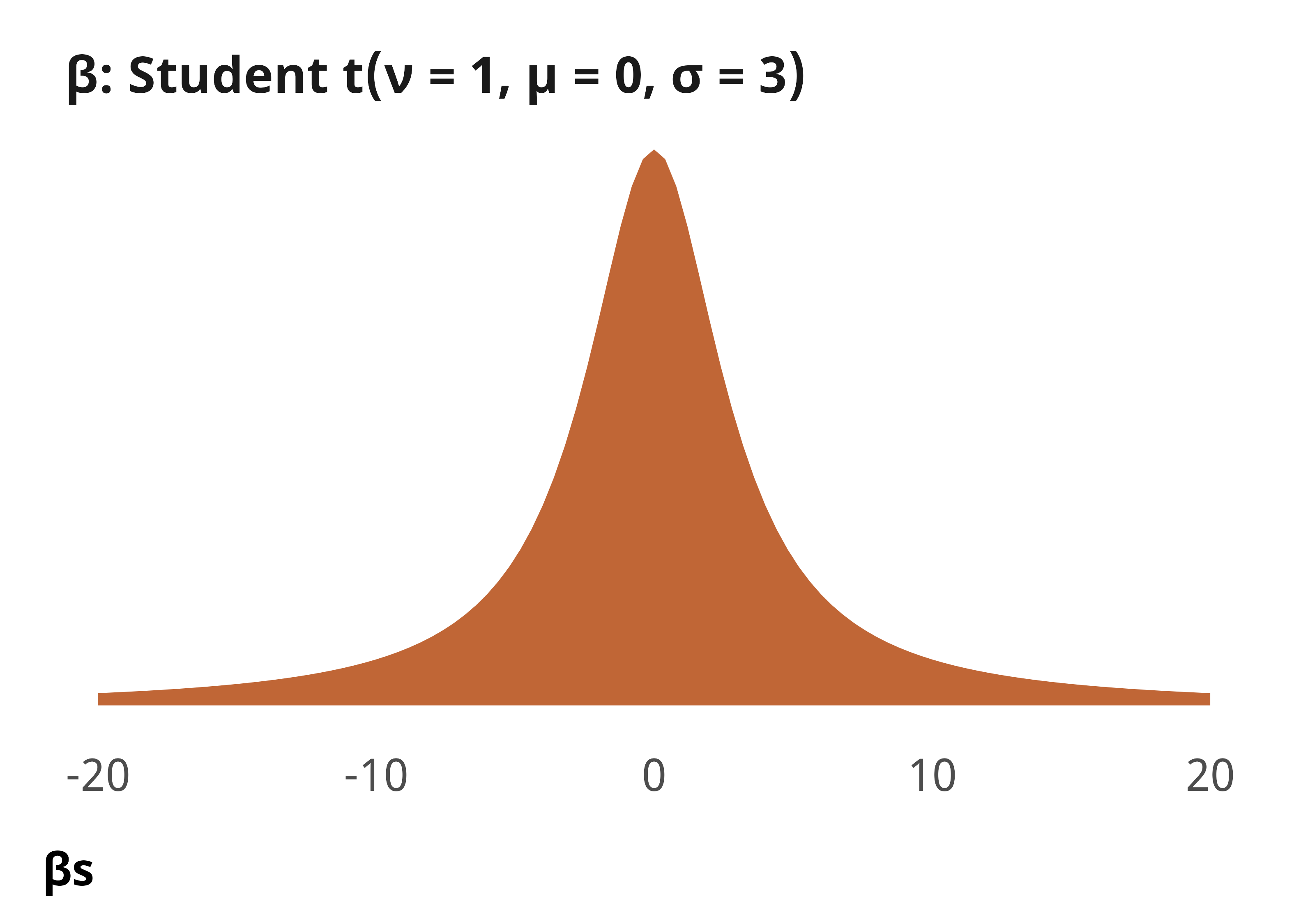
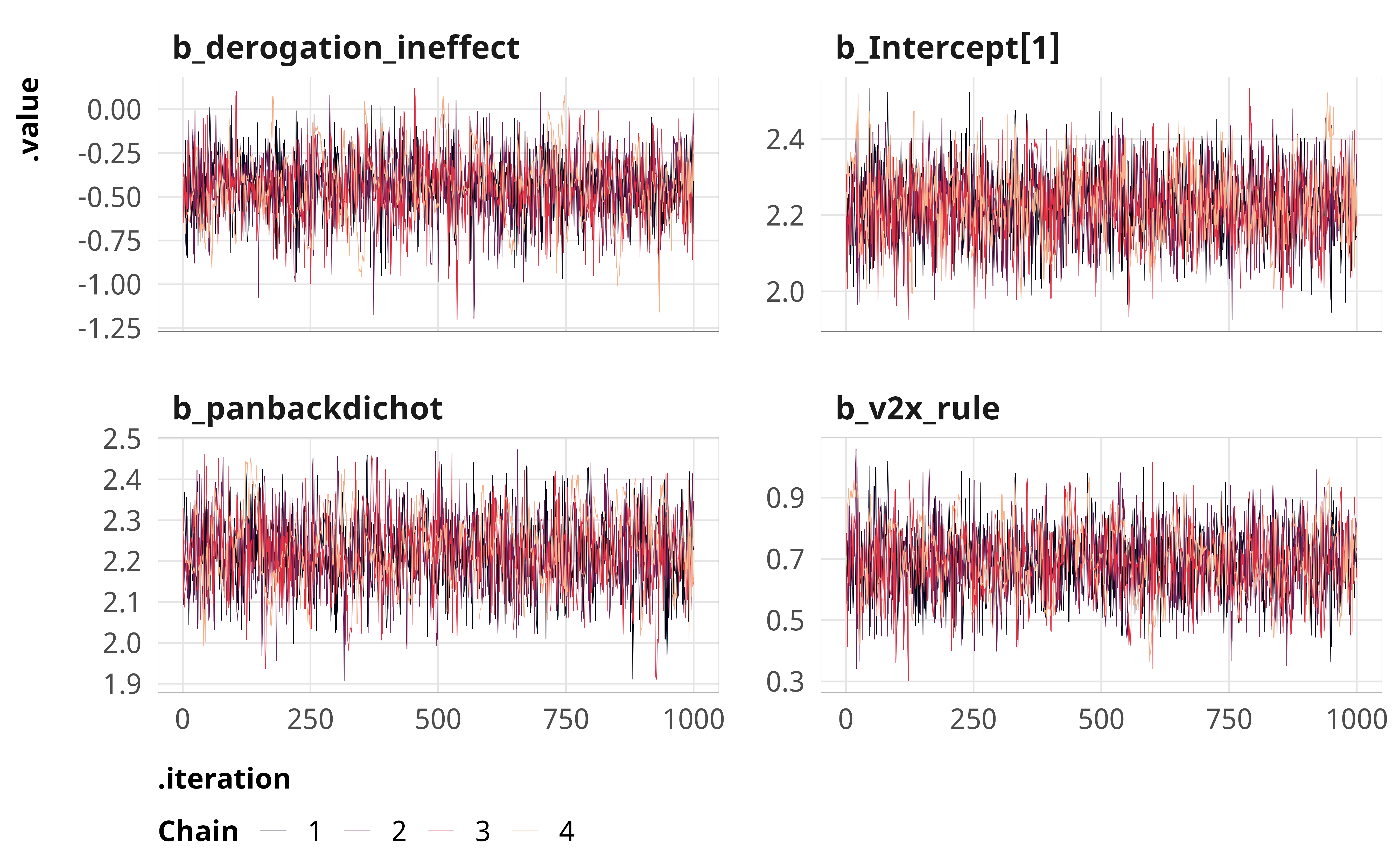
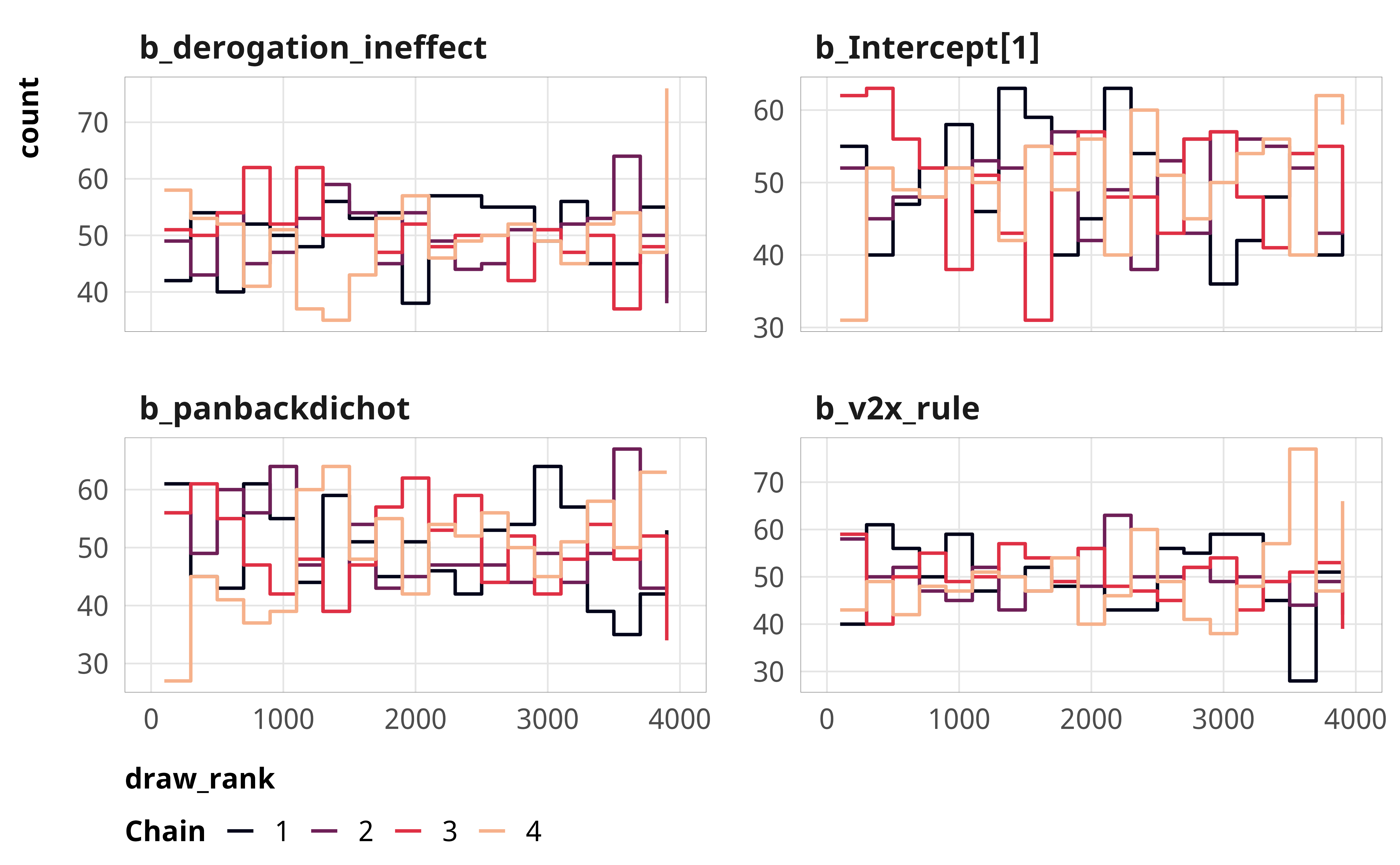
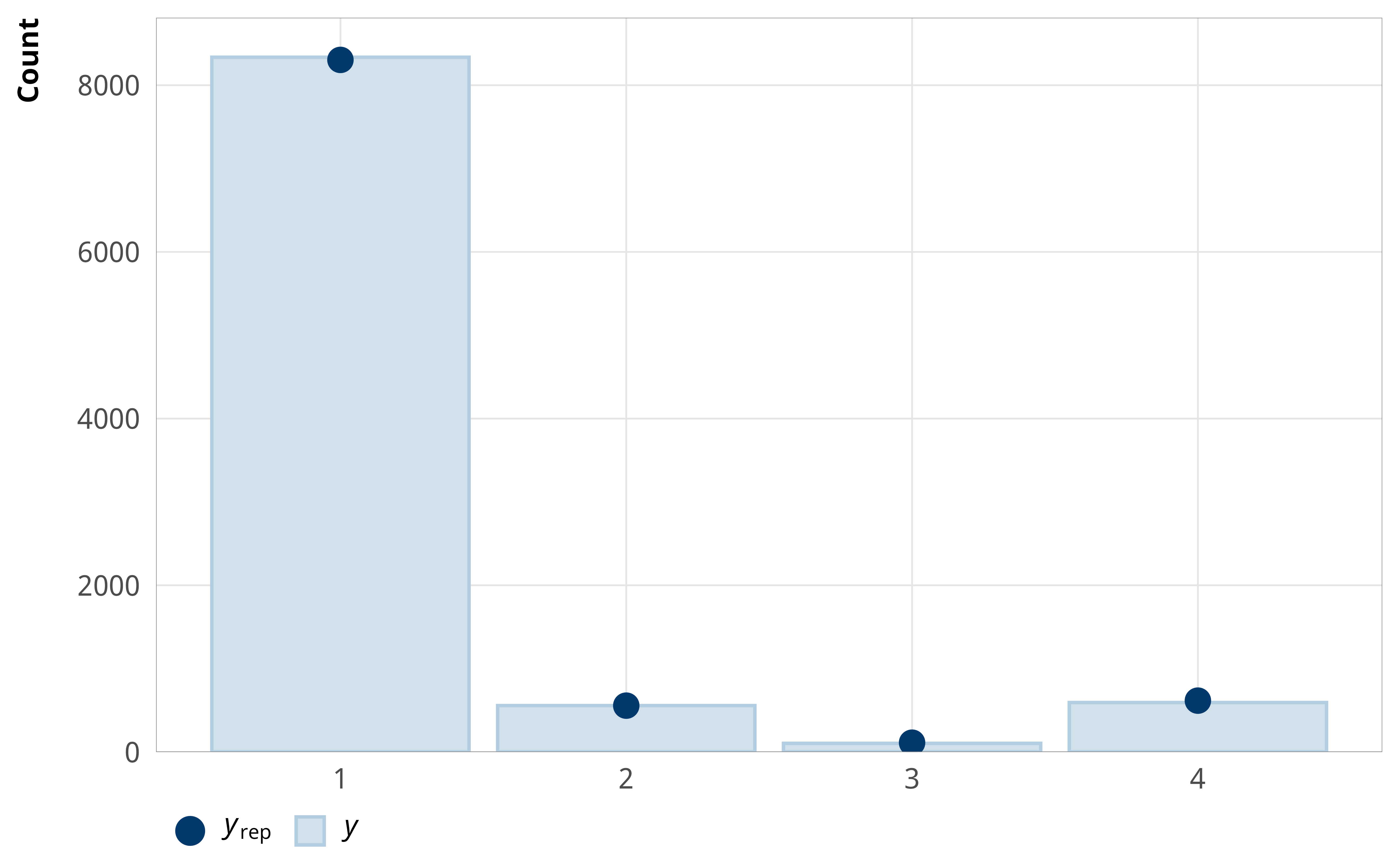
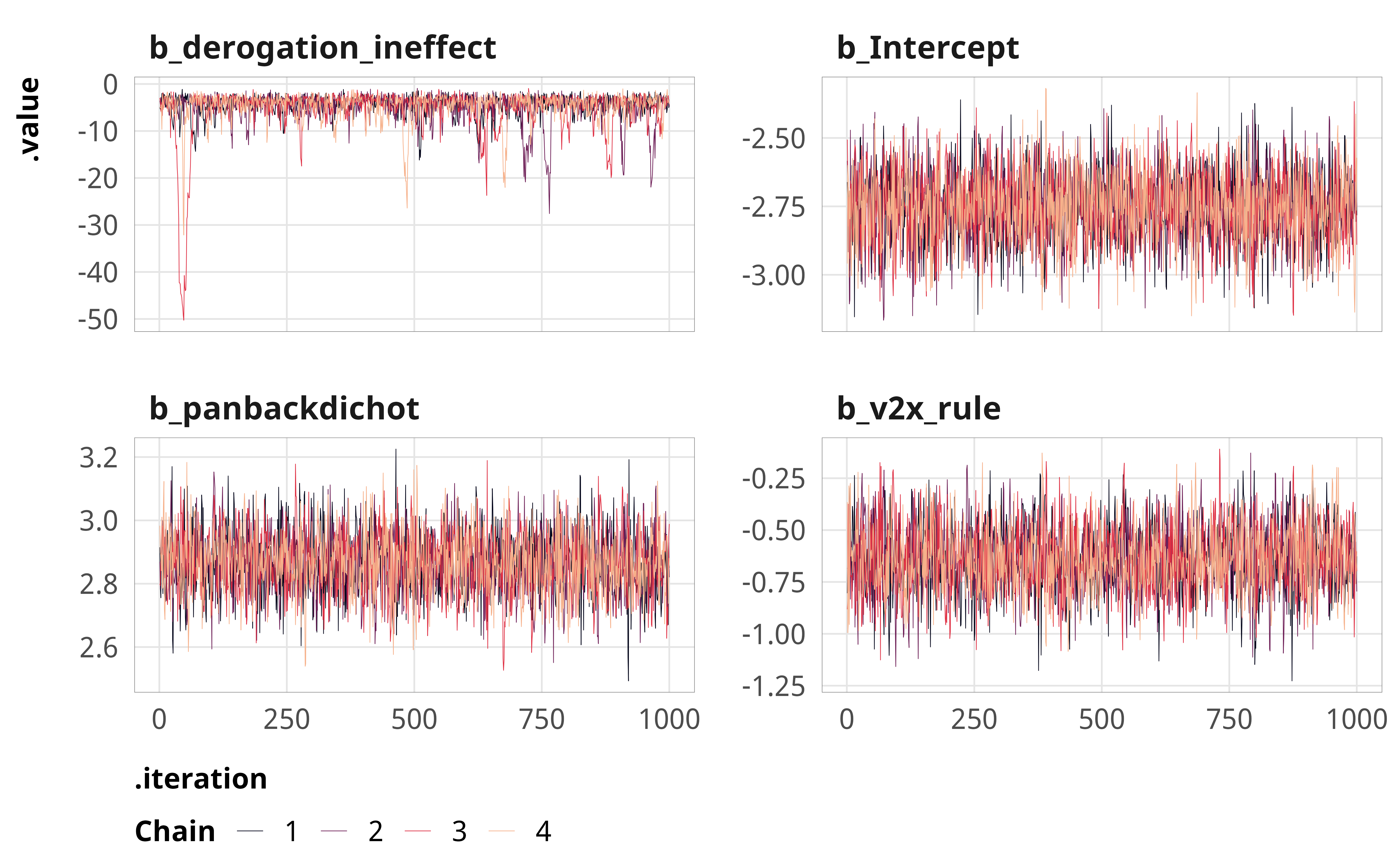
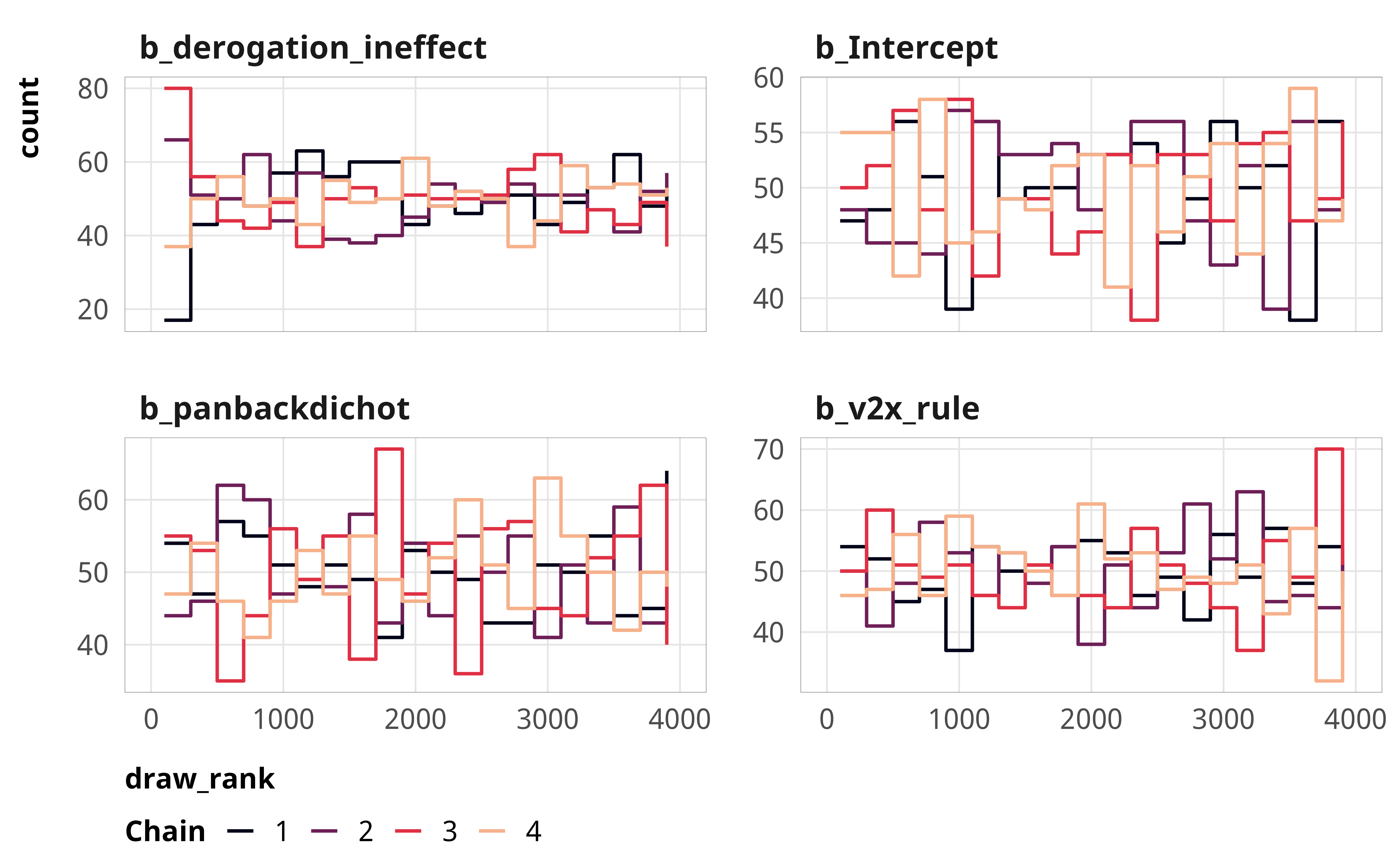
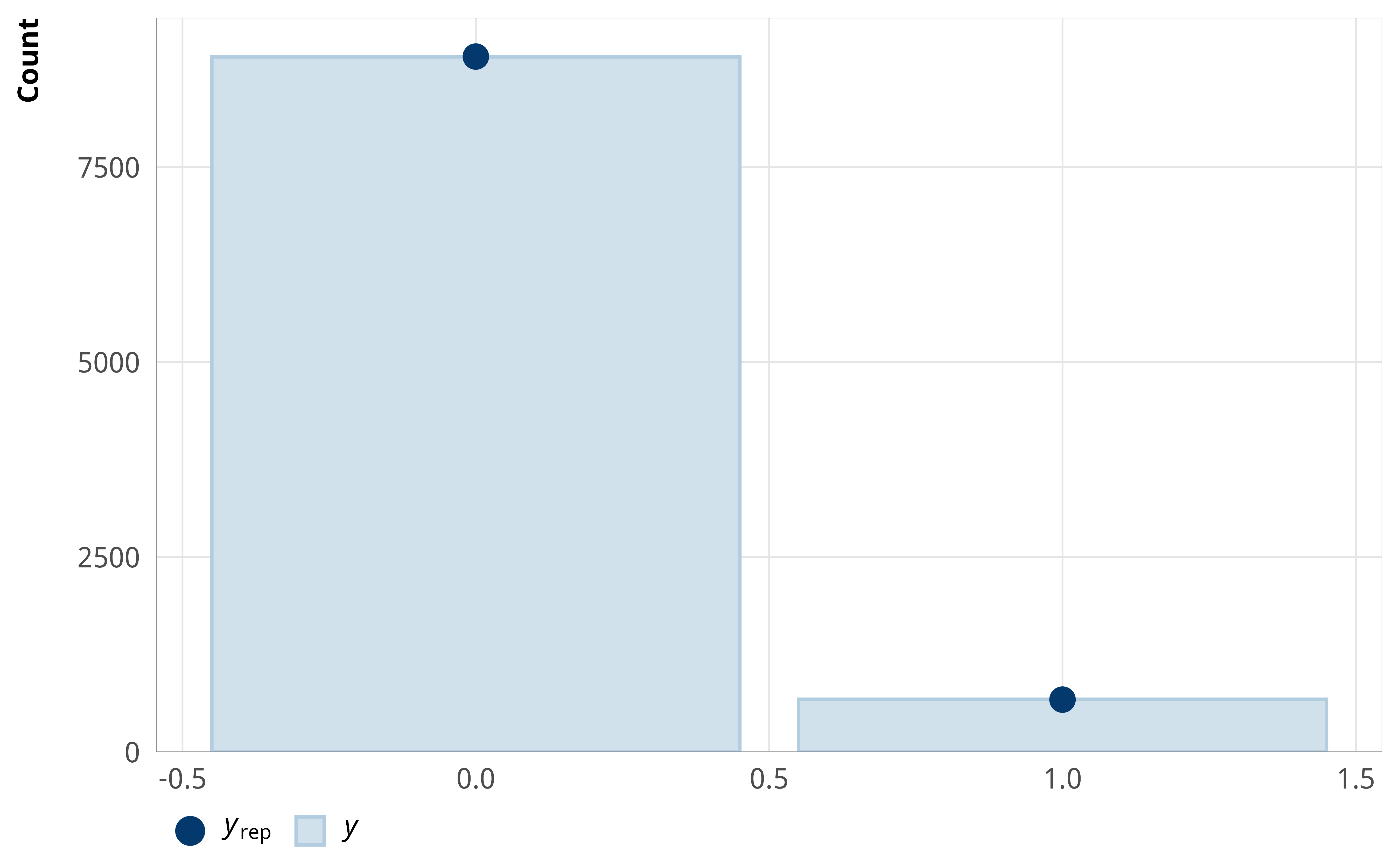
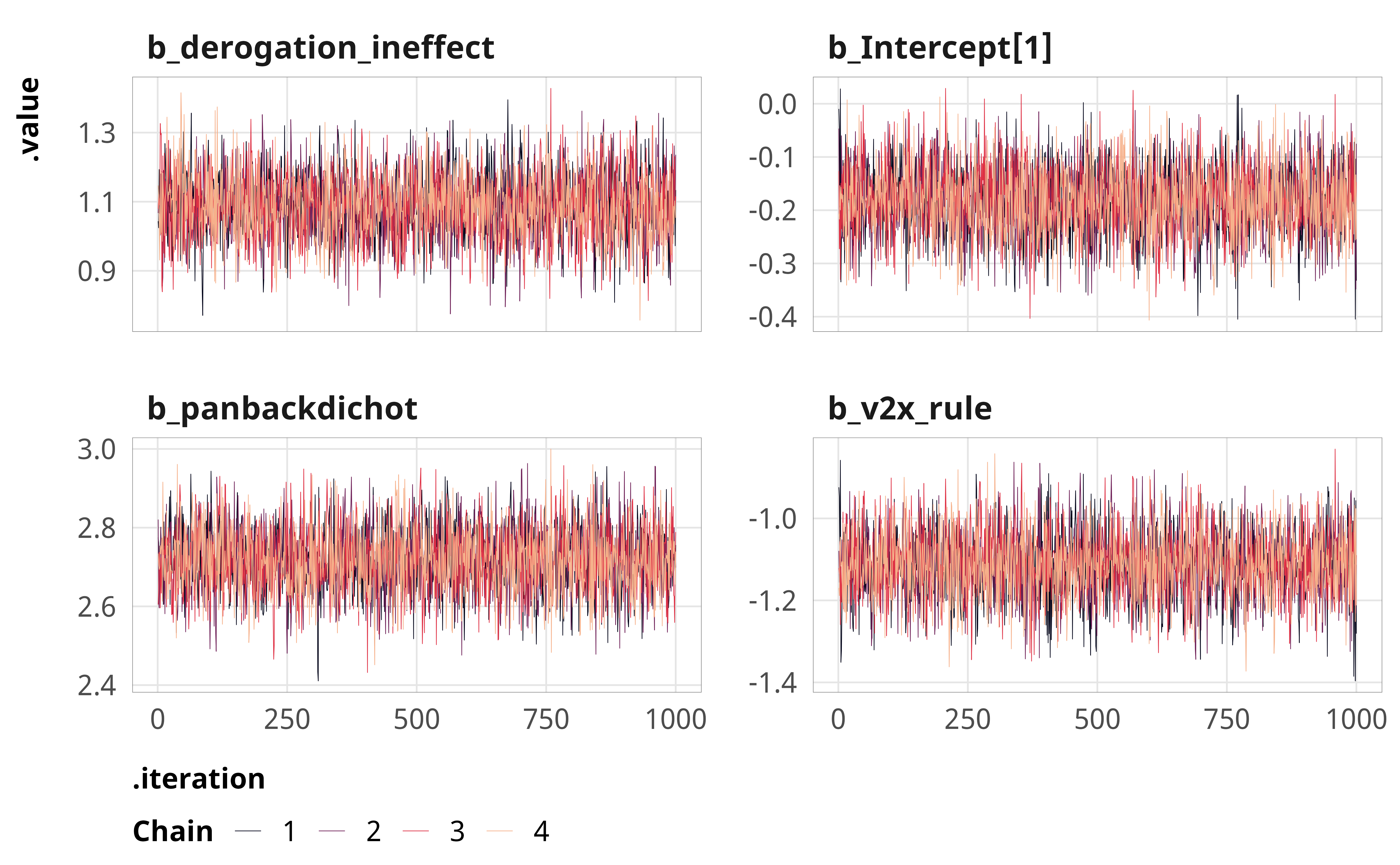
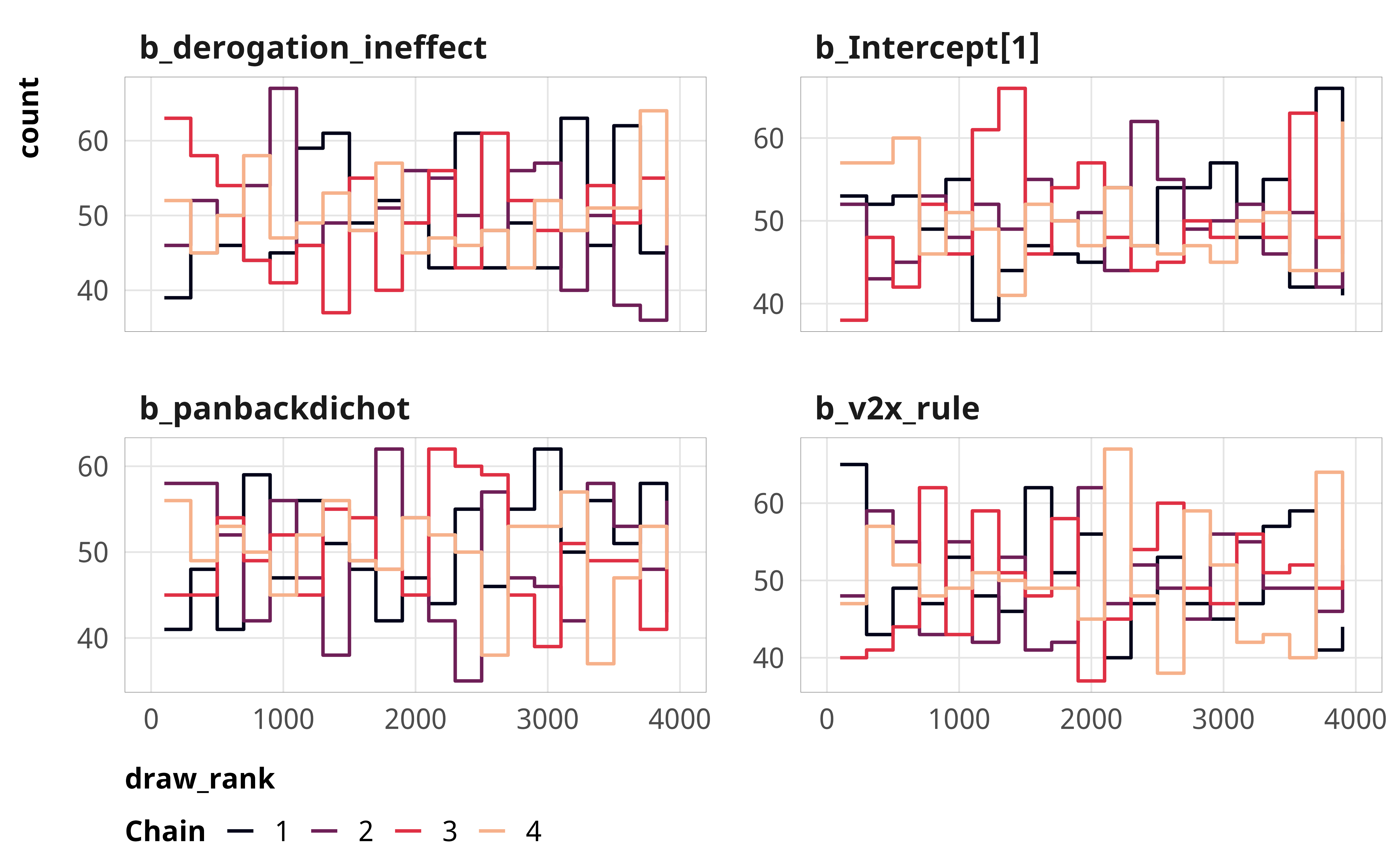
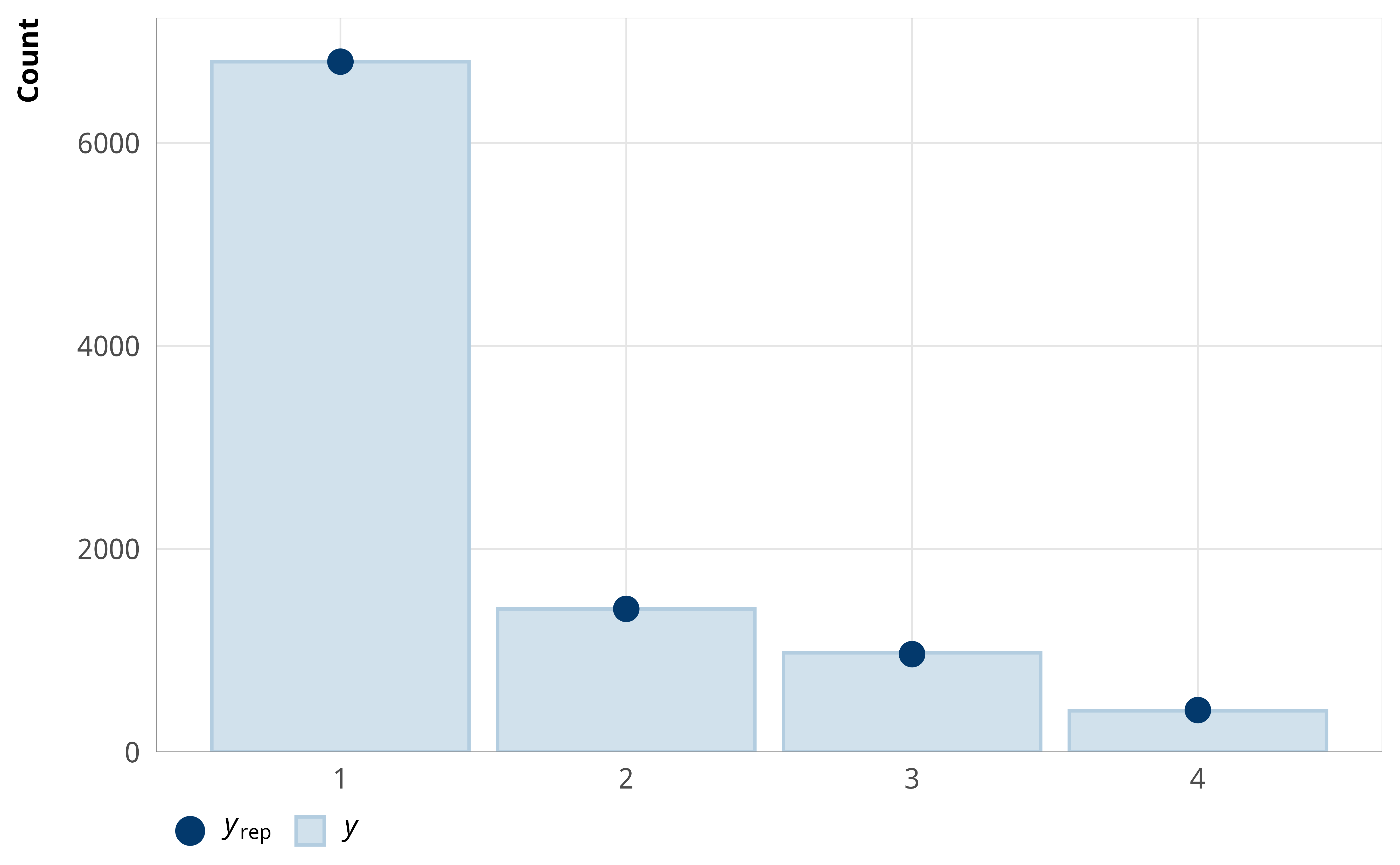
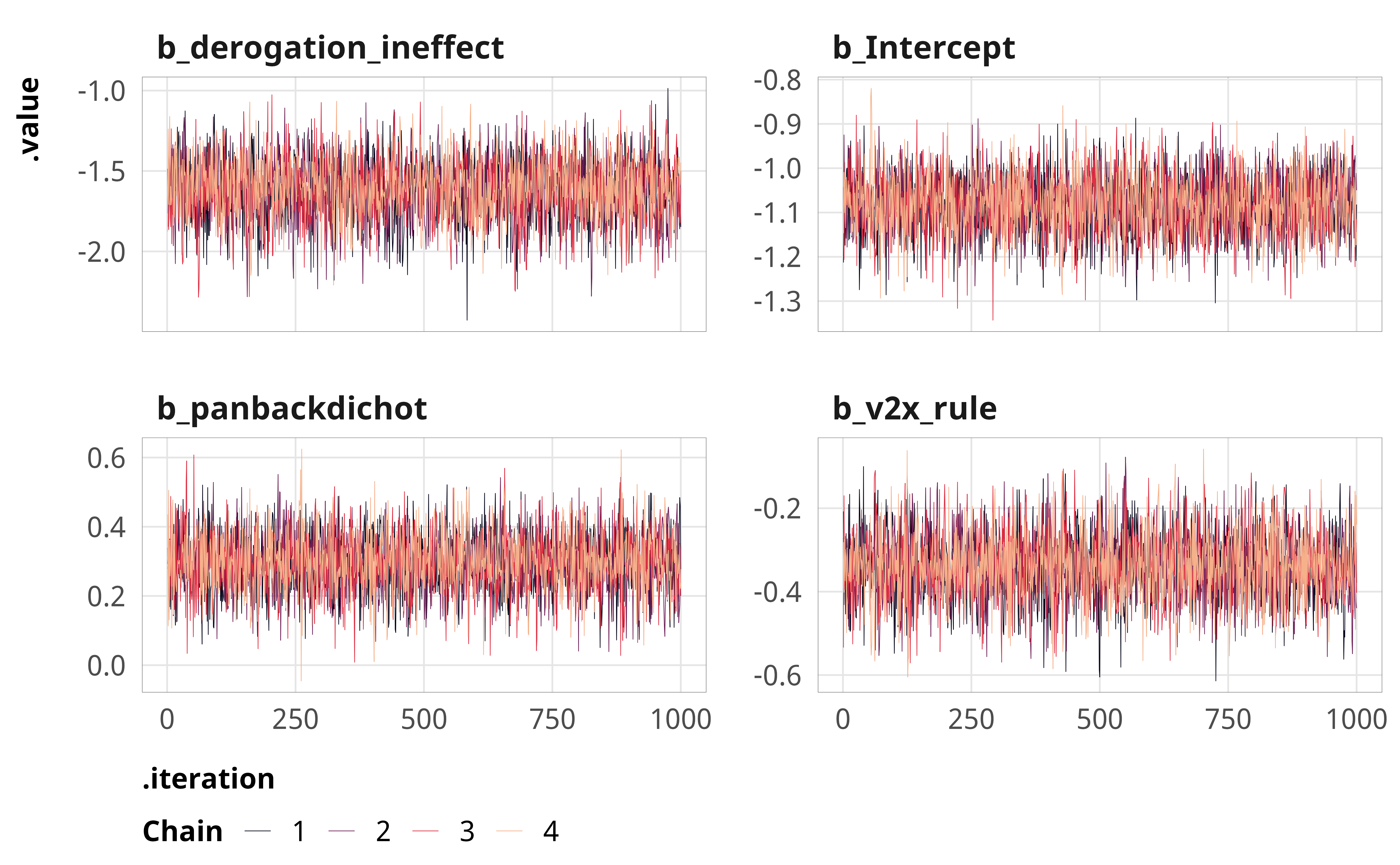
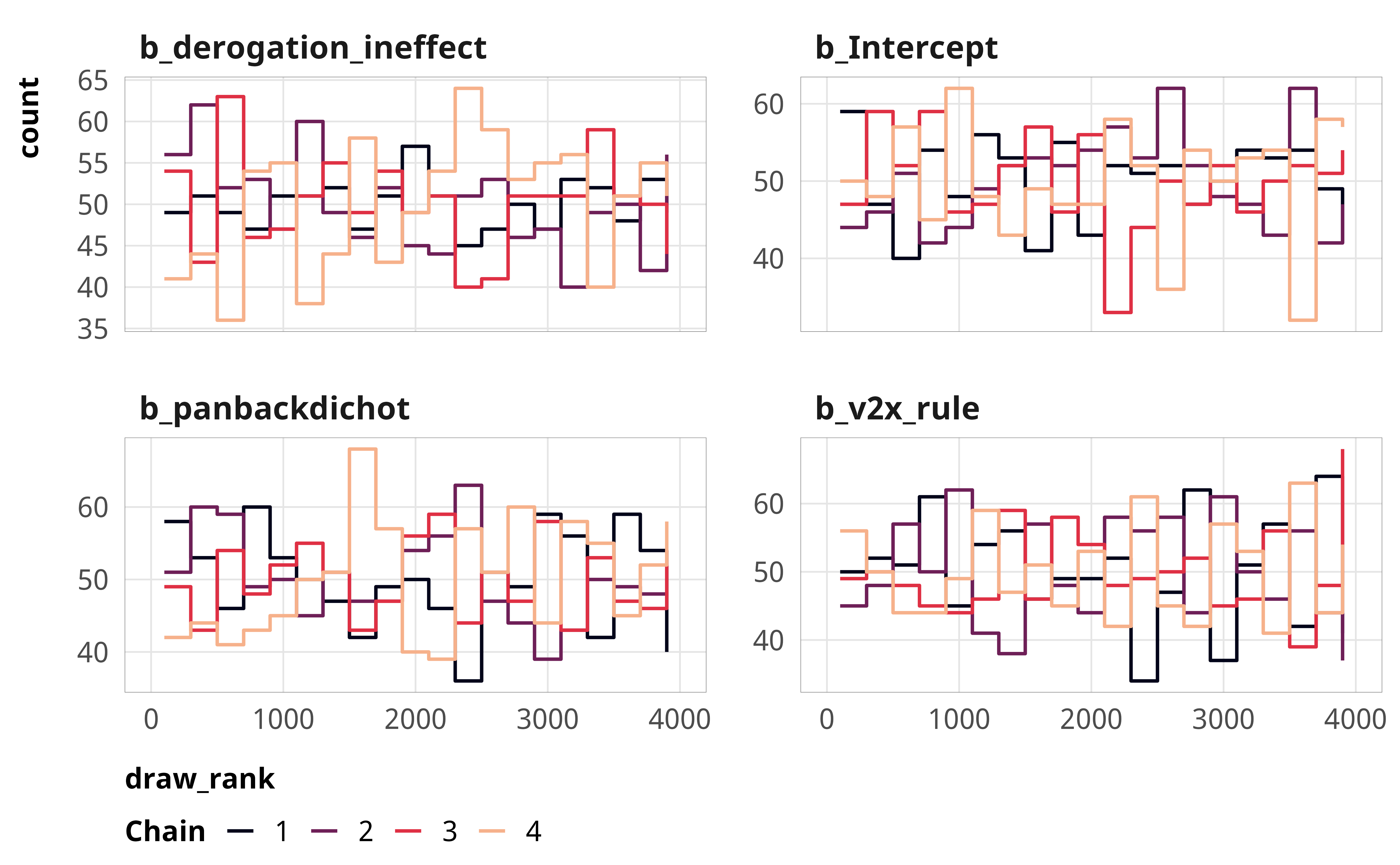
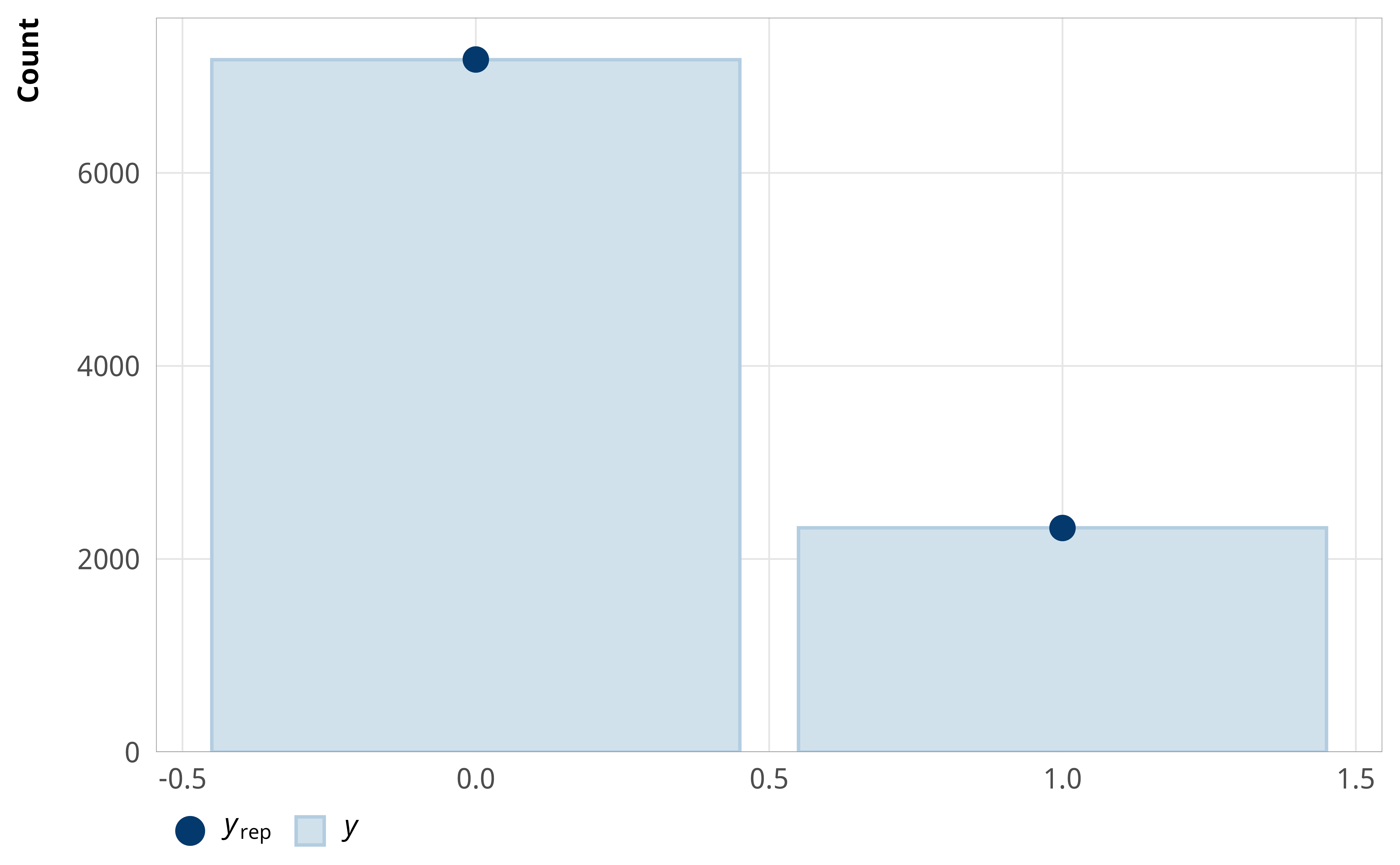
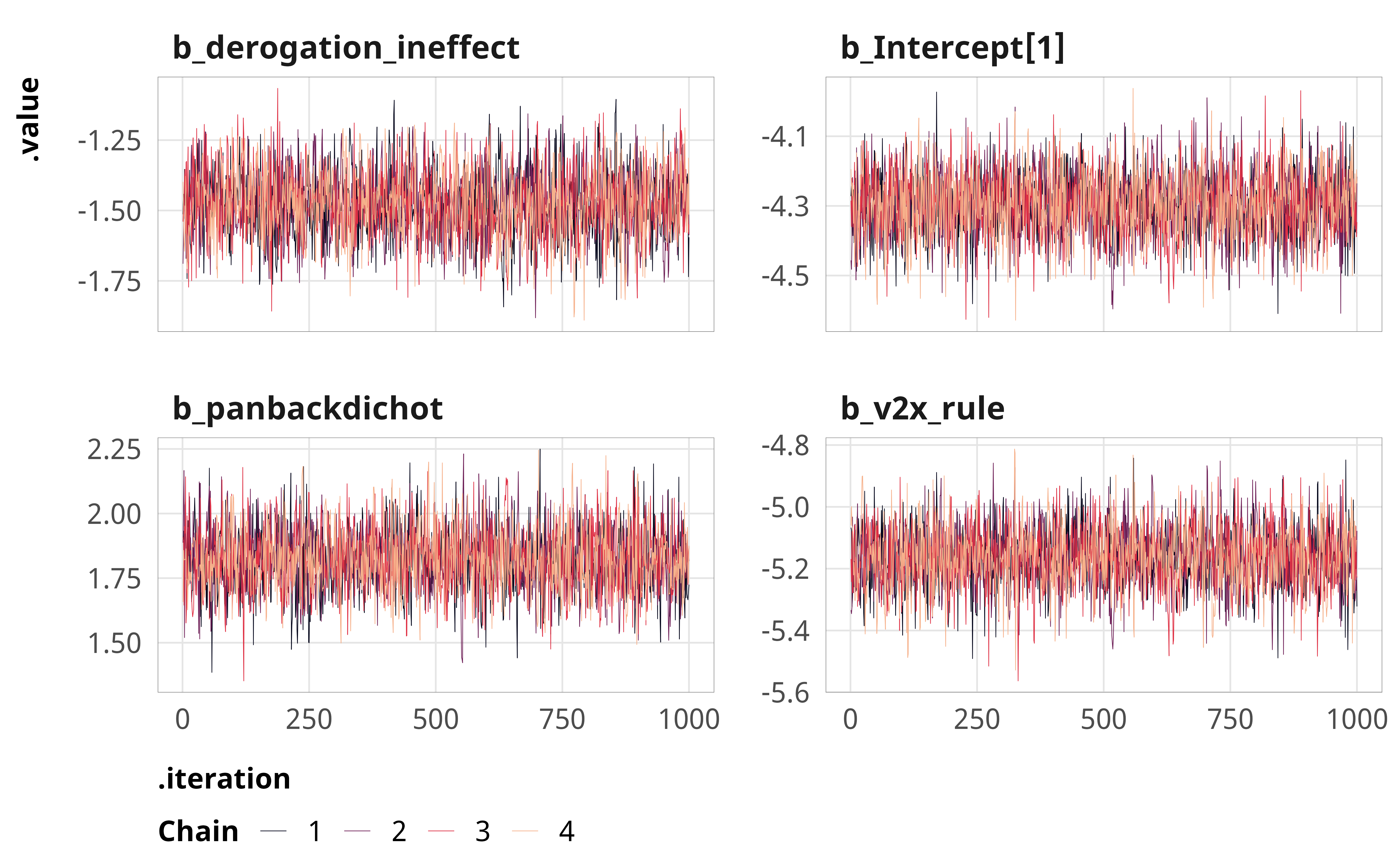
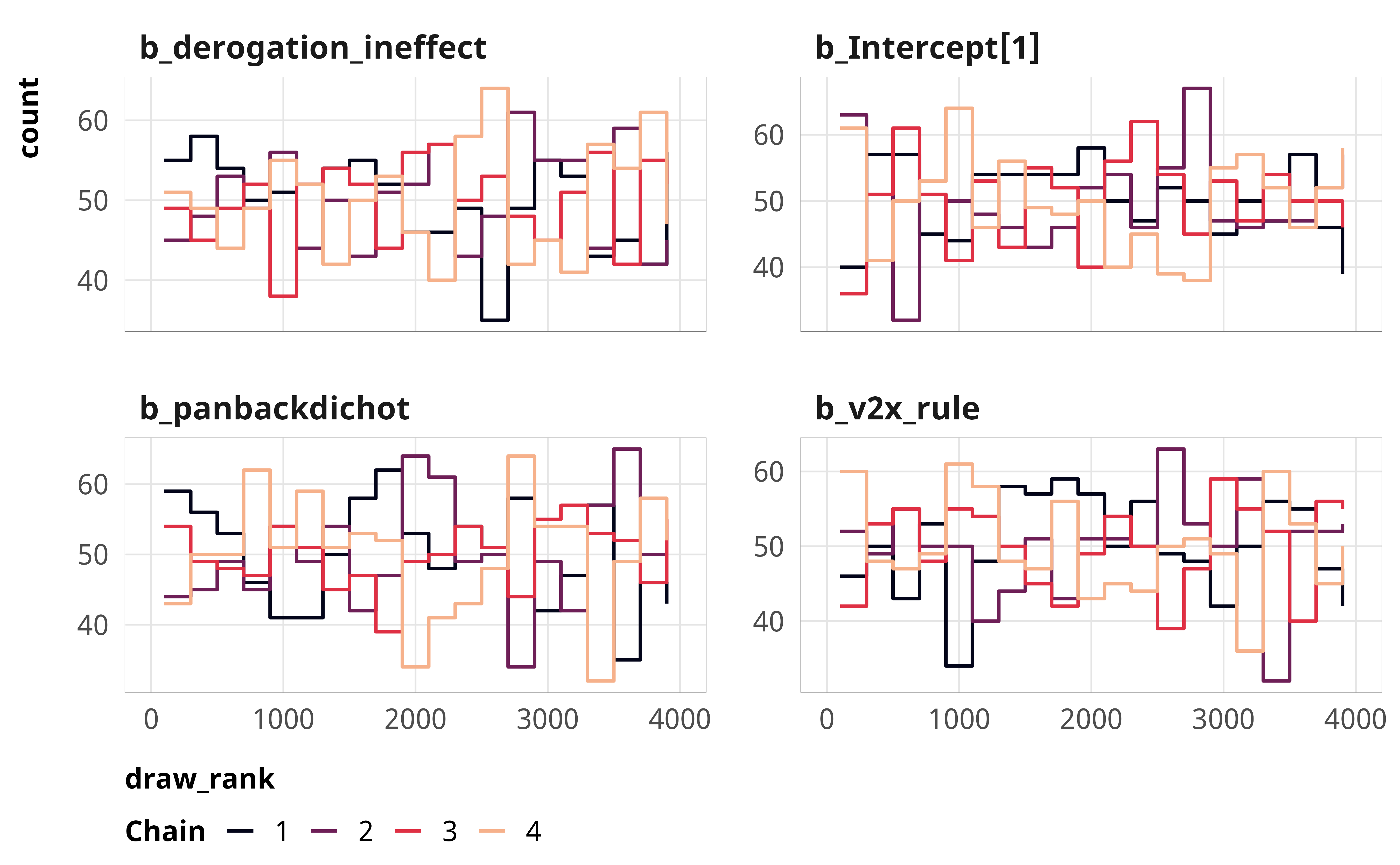
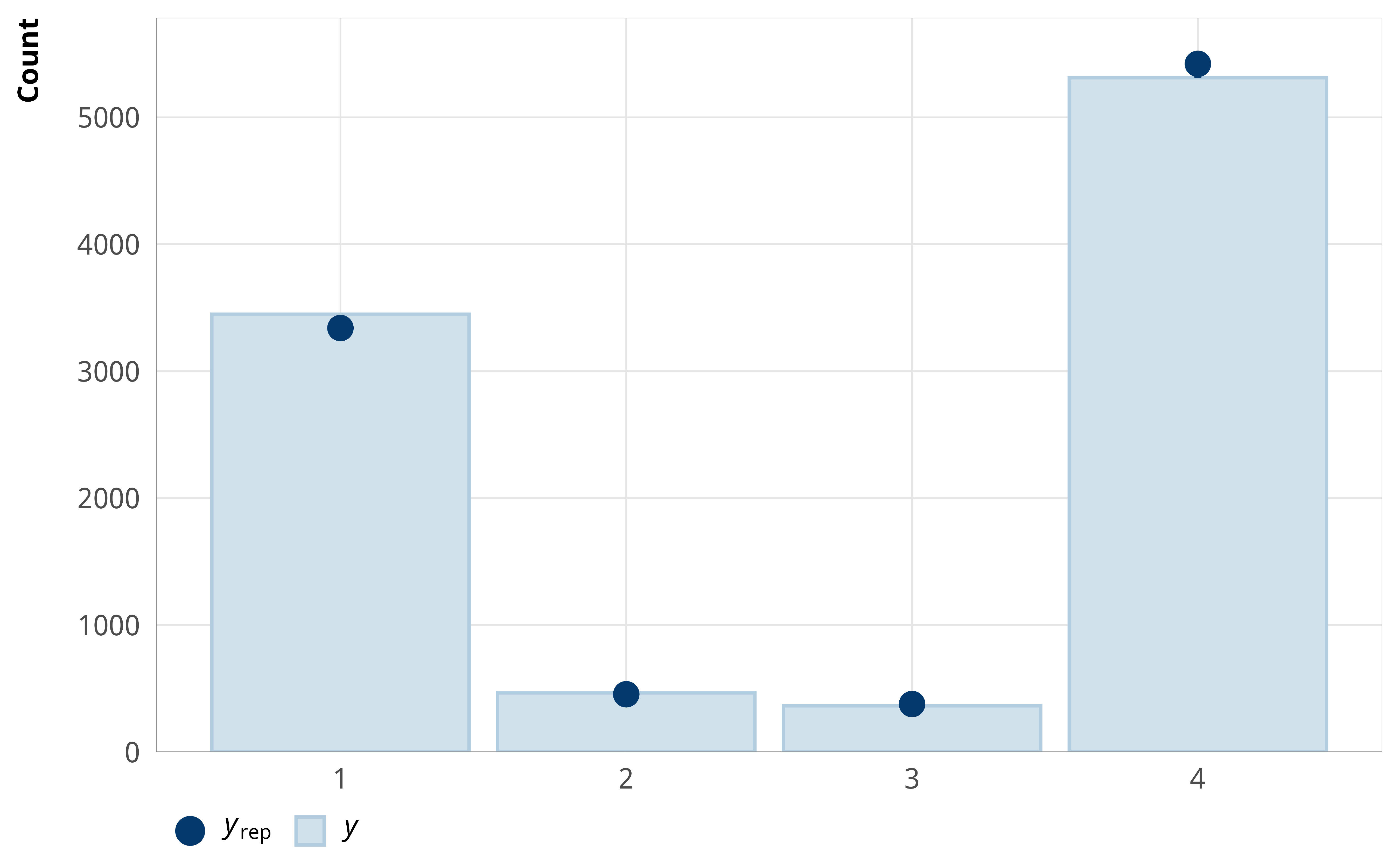
--- title: "Explaining human rights violations" format: html: code-fold: true --- ```{r} #| label: setup #| include: false :: opts_chunk$ set (fig.width = 6 , fig.height = (6 * 0.618 ), out.width = "80%" ,fig.align = "center" , fig.retina = 3 ,collapse = TRUE options (digits = 3 , width = 120 , dplyr.summarise.inform = FALSE )``` ```{r} #| label: libraries-data #| warning: false #| message: false library (tidyverse)library (tidybayes)library (modelsummary)library (marginaleffects)library (scales)library (glue)library (ggtext)library (patchwork)library (ggh4x)library (tinytable)library (targets)tar_config_set (store = here:: here ("_targets" ),script = here:: here ("_targets.R" )tar_load (c (m_hr, m_tbl_hr))invisible (list2env (tar_read (graphic_functions), .GlobalEnv))invisible (list2env (tar_read (diagnostic_functions), .GlobalEnv))invisible (list2env (tar_read (helper_functions), .GlobalEnv))invisible (list2env (tar_read (modelsummary_functions), .GlobalEnv))set_annotation_fonts ()``` # Model details ## Formal model specification \\ \\ [ 0.75em ] \\ \\ [ \text{PanBack (binary)}_{it} \times \text{Derogation in effect}_{it} ] + \\ \\ \\ \\ [ 0.75em ] \\ \\ ## Priors ```{r} #| label: figure-prior #| fig-cap: "Density plot of prior distribution for model parameters" #| fig-width: 3.5 #| fig-height: 2.5 #| out-width: "50%" ggplot () + stat_function (geom = "area" ,fun = ~ extraDistr:: dlst (., df = 1 , mu = 0 , sigma = 3 ),fill = clrs[2 ]+ xlim (c (- 20 , 20 )) + labs (x = "βs" ) + facet_wrap (vars ("β: Student t(ν = 1, µ = 0, σ = 3)" )) + theme_pandem (prior = TRUE )``` ## Simplified R code ```r brm (bf (outcome ~ derogation_ineffect* panbackdichot + + cumulative_cases_z + + cumulative_deaths_z + + year_week_num),family = cumulative (),prior = c (prior (student_t (1 , 0 , 3 ), class = Intercept),prior (student_t (1 , 0 , 3 ), class = b)),``` ## Model evaluation ```{r} <- c ("b_Intercept[1]" , "b_derogation_ineffect" , "b_panbackdichot" , "b_v2x_rule" )<- c ("b_Intercept" , "b_derogation_ineffect" , "b_panbackdichot" , "b_v2x_rule" )``` ### Discriminatory policy ```{r} plot_trace (m_hr$ m_hr_discrim, params_to_show)``` ```{r} plot_trank (m_hr$ m_hr_discrim, params_to_show)``` ```{r} plot_pp (m_hr$ m_hr_discrim)``` ### Non-derogable rights ```{r} plot_trace (m_hr$ m_hr_ndrights, params_to_show_logit)``` ```{r} plot_trank (m_hr$ m_hr_ndrights, params_to_show_logit)``` ```{r} plot_pp (m_hr$ m_hr_ndrights)``` ### Abusive enforcement ```{r} plot_trace (m_hr$ m_hr_abusive, params_to_show)``` ```{r} plot_trank (m_hr$ m_hr_abusive, params_to_show)``` ```{r} plot_pp (m_hr$ m_hr_abusive)``` ### No time limits ```{r} plot_trace (m_hr$ m_hr_nolimit, params_to_show_logit)``` ```{r} plot_trank (m_hr$ m_hr_nolimit, params_to_show_logit)``` ```{r} plot_pp (m_hr$ m_hr_nolimit)``` ### Media restrictions ```{r} plot_trace (m_hr$ m_hr_media, params_to_show)``` ```{r} plot_trank (m_hr$ m_hr_media, params_to_show)``` ```{r} plot_pp (m_hr$ m_hr_media)``` # Results ## Predictions ```{r} #| label: calc-preds-hr # Discriminatory policy <- calc_preds (m_hr$ m_hr_discrim)<- calc_preds_details (preds_hr_discrim)<- calc_preds_diffs (preds_hr_discrim)<- calc_preds_diffs_details (diffs_hr_discrim)# Non-derogable rights <- calc_preds (m_hr$ m_hr_ndrights)<- bind_rows (|> mutate (.category = "Major" ),|> mutate (.category = "None" ) |> mutate (.epred = 1 - .epred)|> mutate (.category = factor (.category, levels = c ("None" , "Major" ), ordered = TRUE ))<- calc_preds_details (preds_hr_ndrights_plot)<- calc_preds_diffs (preds_hr_ndrights_plot)<- calc_preds_diffs_details (diffs_hr_ndrights)# Abusive enforcement <- calc_preds (m_hr$ m_hr_abusive)<- calc_preds_details (preds_hr_abusive)<- calc_preds_diffs (preds_hr_abusive)<- calc_preds_diffs_details (diffs_hr_abusive)# Time limits <- calc_preds (m_hr$ m_hr_nolimit)<- bind_rows (|> mutate (.category = "Moderate" ),|> mutate (.category = "None" ) |> mutate (.epred = 1 - .epred)|> mutate (.category = factor (.category, levels = c ("None" , "Moderate" ), ordered = TRUE ))<- calc_preds_details (preds_hr_nolimit_plot)<- calc_preds_diffs (preds_hr_nolimit_plot)<- calc_preds_diffs_details (diffs_hr_nolimit)# Media restrictions <- calc_preds (m_hr$ m_hr_media)<- calc_preds_details (preds_hr_media)<- calc_preds_diffs (preds_hr_media)<- calc_preds_diffs_details (diffs_hr_media)``` ```{r} #| label: figure-hr-preds #| fig-cap: Predicted probabilities of violating human rights across states with low and high risks of democratic backsliding and derogation status #| fig-width: 9.75 #| fig-height: 8.75 #| out-width: 100% #| lightbox: true <- ggplot (preds_hr_discrim, aes (x = .draw, y = .epred)) + geom_area (aes (fill = .category), position = position_stack ()) + geom_label (data = calc_fuzzy_labs (preds_hr_discrim_details),aes (x = x, y = y, label = prob_ci_nice, hjust = hjust),fill = scales:: alpha ("white" , 0.4 ), label.size = 0 ,fontface = "bold" , size = 8 , size.unit = "pt" + scale_x_continuous (breaks = NULL , expand = c (0 , 0 )) + scale_y_continuous (labels = label_percent (), expand = c (0 , 0 )) + scale_fill_manual (values = clrs[c (7 , 4 , 2 , 1 )]) + labs (x = NULL , y = "Cumulative \n probabilities" ,fill = "Discriminatory policy" , tag = "A" + facet_nested_wrap (vars (panbackdichot, derogation_ineffect),strip = nested_settings,nrow = 1 + theme_pandem () + <- ggplot (preds_hr_ndrights_plot, aes (x = .draw, y = .epred)) + geom_area (aes (fill = .category), position = position_stack ()) + geom_label (data = calc_fuzzy_labs (preds_hr_ndrights_details),aes (x = x, y = y, label = prob_ci_nice, hjust = hjust),fill = scales:: alpha ("white" , 0.4 ), label.size = 0 ,fontface = "bold" , size = 8 , size.unit = "pt" + scale_x_continuous (breaks = NULL , expand = c (0 , 0 )) + scale_y_continuous (labels = label_percent (), expand = c (0 , 0 )) + scale_fill_manual (values = clrs[c (7 , 1 )]) + labs (x = NULL , y = "Cumulative \n probabilities" ,fill = "Violation of non-derogable rights" , tag = "B" + facet_nested_wrap (vars (panbackdichot, derogation_ineffect),strip = nested_settings,nrow = 1 + theme_pandem () + <- ggplot (preds_hr_abusive, aes (x = .draw, y = .epred)) + geom_area (aes (fill = .category), position = position_stack ()) + geom_label (data = calc_fuzzy_labs (preds_hr_abusive_details),aes (x = x, y = y, label = prob_ci_nice, hjust = hjust),fill = scales:: alpha ("white" , 0.4 ), label.size = 0 ,fontface = "bold" , size = 8 , size.unit = "pt" + scale_x_continuous (breaks = NULL , expand = c (0 , 0 )) + scale_y_continuous (labels = label_percent (), expand = c (0 , 0 )) + scale_fill_manual (values = clrs[c (7 , 4 , 2 , 1 )]) + labs (x = NULL , y = "Cumulative \n probabilities" ,fill = "Abusive enforcement" , tag = "C" + facet_nested_wrap (vars (panbackdichot, derogation_ineffect),strip = nested_settings,nrow = 1 + theme_pandem () + <- ggplot (preds_hr_nolimit_plot, aes (x = .draw, y = .epred)) + geom_area (aes (fill = .category), position = position_stack ()) + geom_label (data = calc_fuzzy_labs (preds_hr_nolimit_details),aes (x = x, y = y, label = prob_ci_nice, hjust = hjust),fill = scales:: alpha ("white" , 0.4 ), label.size = 0 ,fontface = "bold" , size = 8 , size.unit = "pt" + scale_x_continuous (breaks = NULL , expand = c (0 , 0 )) + scale_y_continuous (labels = label_percent (), expand = c (0 , 0 )) + scale_fill_manual (values = clrs[c (7 , 2 )]) + labs (x = NULL , y = "Cumulative \n probabilities" ,fill = "No time limited measures" , tag = "D" + facet_nested_wrap (vars (panbackdichot, derogation_ineffect),strip = nested_settings,nrow = 1 + theme_pandem () + <- ggplot (preds_hr_media, aes (x = .draw, y = .epred)) + geom_area (aes (fill = .category), position = position_stack ()) + geom_label (data = calc_fuzzy_labs (preds_hr_media_details),aes (x = x, y = y, label = prob_ci_nice, hjust = hjust),fill = scales:: alpha ("white" , 0.4 ), label.size = 0 ,fontface = "bold" , size = 8 , size.unit = "pt" + scale_x_continuous (breaks = NULL , expand = c (0 , 0 )) + scale_y_continuous (labels = label_percent (), expand = c (0 , 0 )) + scale_fill_manual (values = clrs[c (7 , 4 , 2 , 1 )]) + labs (x = NULL , y = "Cumulative \n probabilities" ,fill = "Media restrictions" , tag = "E" + facet_nested_wrap (vars (panbackdichot, derogation_ineffect),strip = nested_settings,nrow = 1 + theme_pandem () + <- " AID FIG BIE HI# CI# " + p2 + p3 + p4 + p5 + line_divider + line_divider + line_divider + line_divider_v + plot_layout (design = layout,heights = c (0.31 , 0.035 , 0.31 , 0.035 , 0.31 ),widths = c (0.94 , 0.02 , 0.94 )+ plot_annotation (caption = str_wrap (glue ("The vertical slices of the bars depict 500 posterior samples;" ,"the fuzziness represents the uncertainty in category boundaries." ,"95% credible intervals are shown as ranges in each category" ,.sep = " " width = 100 theme = theme (plot.caption = element_text (margin = margin (t = 10 ), size = rel (0.7 ),family = "Noto Sans" , face = "plain" ``` ## Complete table of results ```{r} #| label: table-results-full-hr #| tbl-cap: "Complete results from models showing relationship between derogations and human rights violations (H~2~ and H~3~)" <- paste ("Note: Estimates are median posterior log odds from logistic and ordered logistic regression models;" ,"95% credible intervals (highest density posterior interval, or HDPI) in brackets." |> set_names (c ("Discriminatory policy" , "Non-derogable rights" ,"Abusive enforcement" , "No time limits" , "Media restrictions" )) |> modelsummary (estimate = "{estimate}" ,statistic = "[{conf.low}, {conf.high}]" ,coef_map = coef_map,gof_map = gof_map,output = "tinytable" ,fmt = fmt_significant (2 ),notes = notes,width = c (0.2 , rep (0.16 , 5 ))|> style_tt (i = seq (1 , 27 , 2 ), j = 1 , rowspan = 2 , alignv = "t" ) |> style_tt (bootstrap_class = "table table-sm" ``` ## Contrasts ```{r} #| label: figure-restriction-diffs #| fig-cap: Contrasts in predicted probabilities of implementing COVID restrictions across states with low and high risks of democratic backsliding and derogation status #| fig-width: 9.5 #| fig-height: 10 #| out-width: 100% #| lightbox: true <- diffs_hr_discrim |> ggplot (aes (x = .epred, y = fct_rev (.category), color = .category)) + geom_vline (xintercept = 0 , linewidth = 0.25 , linetype = "21" ) + stat_pointinterval () + facet_nested_wrap (vars (panbackdichot, derogation_ineffect), strip = nested_settings_diffs) + scale_x_continuous (labels = label_pp) + scale_color_manual (values = clrs[c (7 , 4 , 2 , 1 )], guide = "none" ) + labs (x = NULL , y = NULL ,title = "Discriminatory policy" , tag = "A" + theme_pandem () + <- diffs_hr_ndrights |> ggplot (aes (x = .epred, y = fct_rev (.category), color = .category)) + geom_vline (xintercept = 0 , linewidth = 0.25 , linetype = "21" ) + stat_pointinterval () + facet_nested_wrap (vars (panbackdichot, derogation_ineffect), strip = nested_settings_diffs) + scale_x_continuous (labels = label_pp) + scale_color_manual (values = clrs[c (7 , 1 )], guide = "none" ) + labs (x = NULL , y = NULL ,title = "Non-derogable rights" , tag = "B" + theme_pandem () + <- diffs_hr_abusive |> ggplot (aes (x = .epred, y = fct_rev (.category), color = .category)) + geom_vline (xintercept = 0 , linewidth = 0.25 , linetype = "21" ) + stat_pointinterval () + facet_nested_wrap (vars (panbackdichot, derogation_ineffect), strip = nested_settings_diffs) + scale_x_continuous (labels = label_pp) + scale_color_manual (values = clrs[c (7 , 4 , 2 , 1 )], guide = "none" ) + labs (x = NULL , y = NULL ,title = "Abusive enforcement" , tag = "C" + theme_pandem () + <- diffs_hr_nolimit |> ggplot (aes (x = .epred, y = fct_rev (.category), color = .category)) + geom_vline (xintercept = 0 , linewidth = 0.25 , linetype = "21" ) + stat_pointinterval () + facet_nested_wrap (vars (panbackdichot, derogation_ineffect), strip = nested_settings_diffs) + scale_x_continuous (labels = label_pp) + scale_color_manual (values = clrs[c (7 , 2 )], guide = "none" ) + labs (x = NULL , y = NULL ,title = "No time limited measures" , tag = "D" + theme_pandem () + <- diffs_hr_media |> ggplot (aes (x = .epred, y = fct_rev (.category), color = .category)) + geom_vline (xintercept = 0 , linewidth = 0.25 , linetype = "21" ) + stat_pointinterval () + facet_nested_wrap (vars (panbackdichot, derogation_ineffect), strip = nested_settings_diffs) + scale_x_continuous (labels = label_pp) + scale_color_manual (values = clrs[c (7 , 4 , 2 , 1 )], guide = "none" ) + labs (x = NULL , y = NULL ,title = "Media restrictions" , tag = "E" + theme_pandem () + + p2 + p3 + p4 + p5 + line_divider + line_divider + line_divider + line_divider_v) + plot_layout (design = layout,heights = c (0.31 , 0.035 , 0.31 , 0.035 , 0.31 ),widths = c (0.94 , 0.02 , 0.94 )+ plot_annotation (caption = str_wrap (glue ("Point shows posterior median;" , " thick lines show 80% credible interval;" ,"thin black lines show 95% credible interval" ,.sep = " " width = 150 theme = theme (plot.caption = element_text (margin = margin (t = 10 ), size = rel (0.7 ),family = "Noto Sans" , face = "plain" ``` ### Discriminatory policy ```{r} make_diffs_tbl (diffs_hr_discrim)``` ### Non-derogable rights ```{r} make_diffs_tbl (diffs_hr_ndrights)``` ### Abusive enforcement ```{r} make_diffs_tbl (diffs_hr_abusive)``` ### No time limits ```{r} make_diffs_tbl (diffs_hr_nolimit)``` ### Media restrictions ```{r} make_diffs_tbl (diffs_hr_media)```