Complete results from models showing predictors of derogations
(H1)
ICCPR action
Derogation filed
Other action
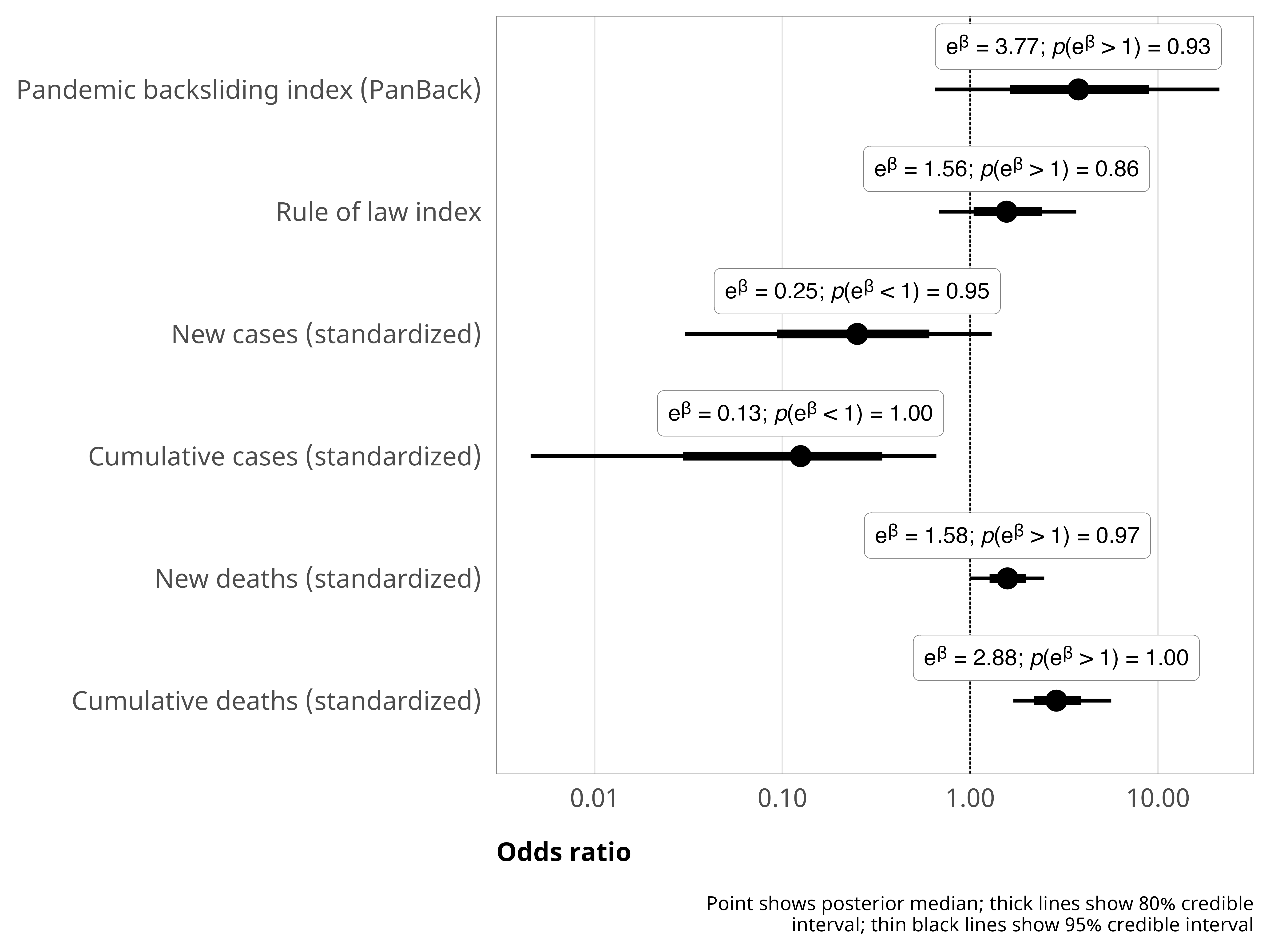
Note: Estimates are median posterior log odds from logistic regression models; 95% credible intervals (highest density posterior interval, or HDPI) in brackets.
Pandemic backsliding (PanBack)
1.33
-2.4
[-0.41, 3.08]
[-7.8, 1.5]
New cases (standardized)
-1.38
-0.42
[-3.29, 0.37]
[-1.89, 0.70]
New deaths (standardized)
0.458
-0.11
[-0.013, 0.893]
[-1.16, 0.72]
Cumulative cases (standardized)
-2.08
-0.59
[-4.96, -0.28]
[-1.44, 0.28]
Cumulative deaths (standardized)
1.06
0.65
[0.51, 1.68]
[-0.15, 1.33]
Rule of law index
0.45
3.2
[-0.40, 1.28]
[1.2, 5.5]
Year-week number
-0.0229
0.010
[-0.0382, -0.0097]
[-0.013, 0.033]
Intercept
-5.1
-8.7
[-6.0, -4.2]
[-11.2, -6.6]
N
9591
9591
\(R^2\)
0.01
0.00
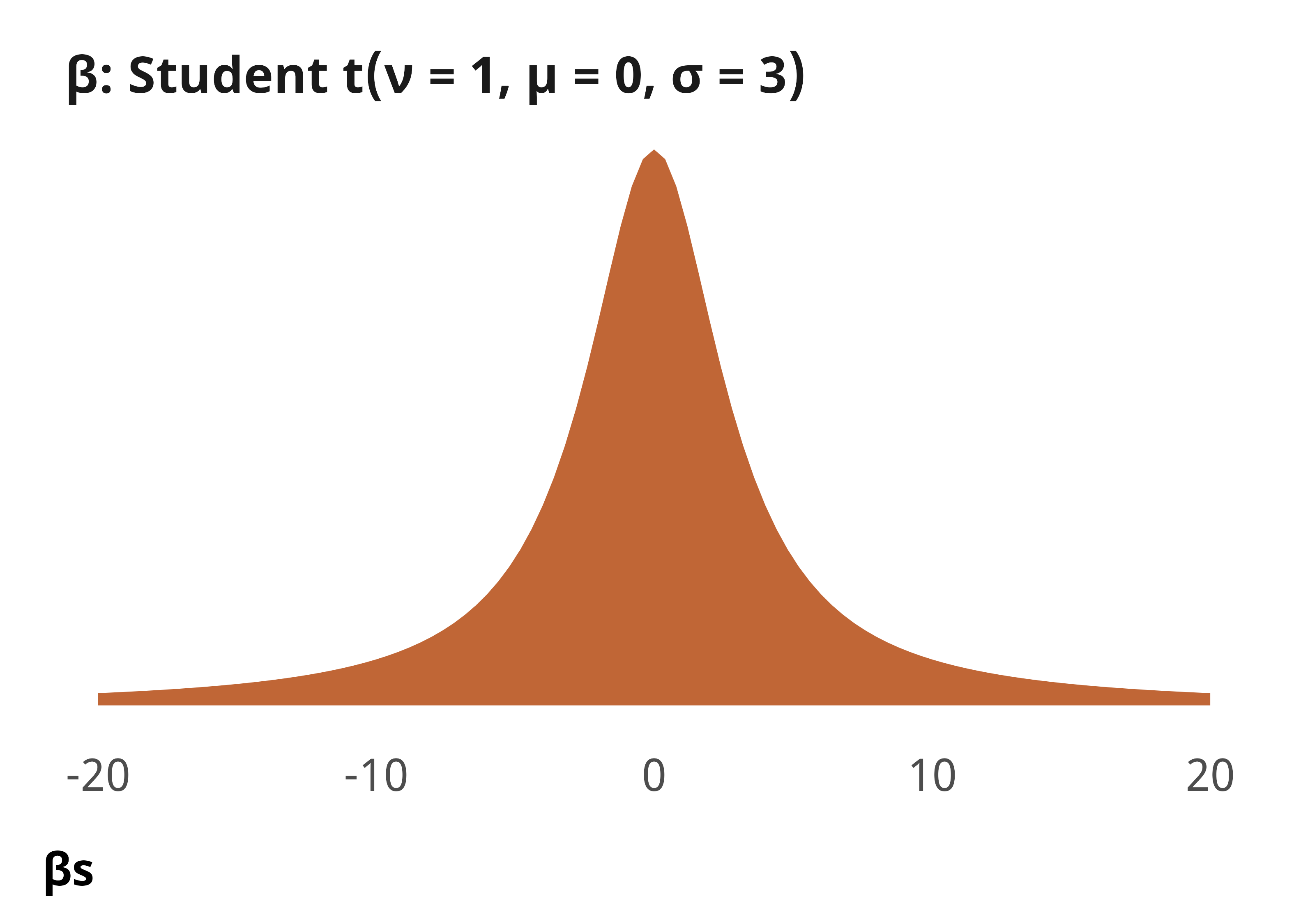
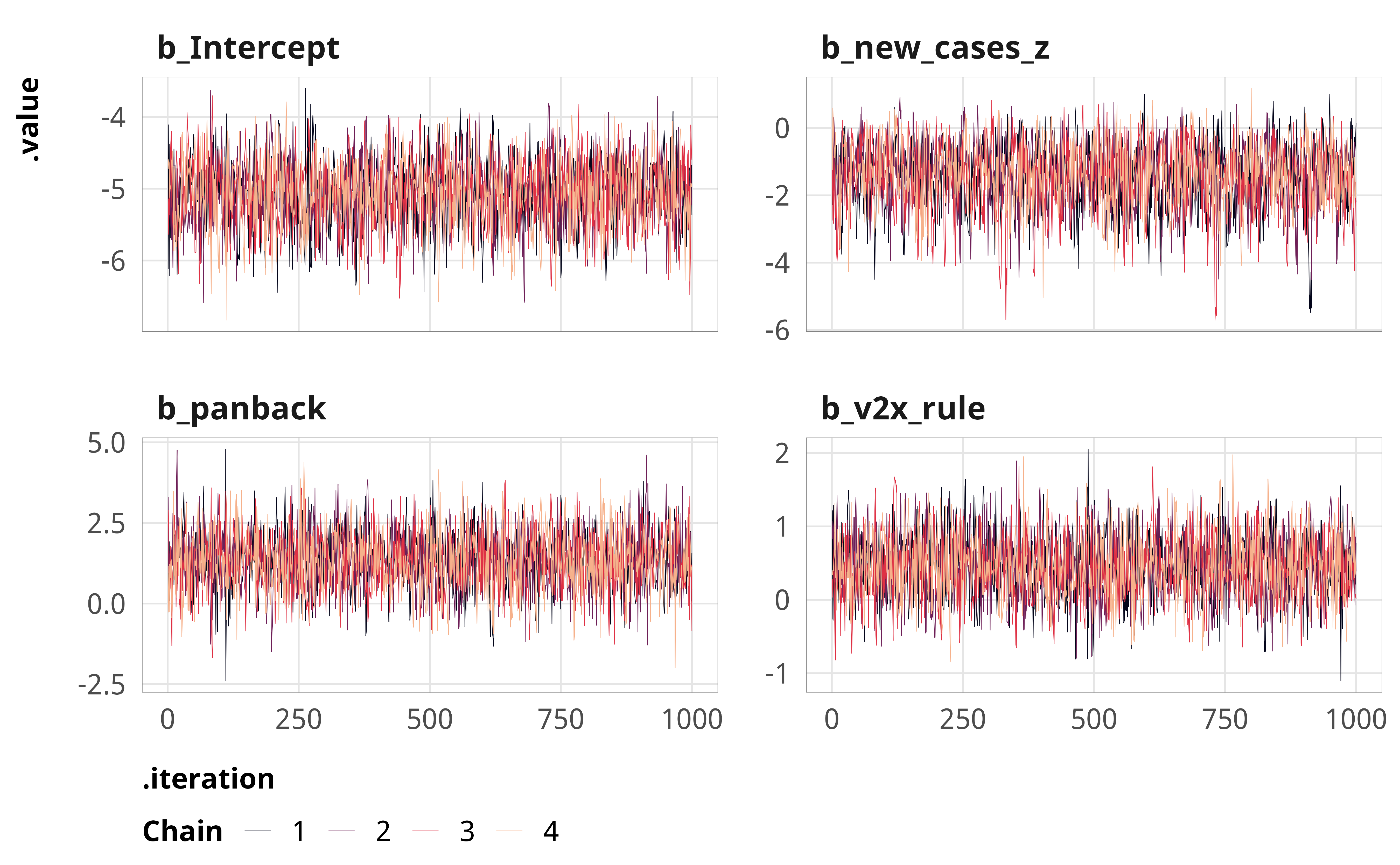
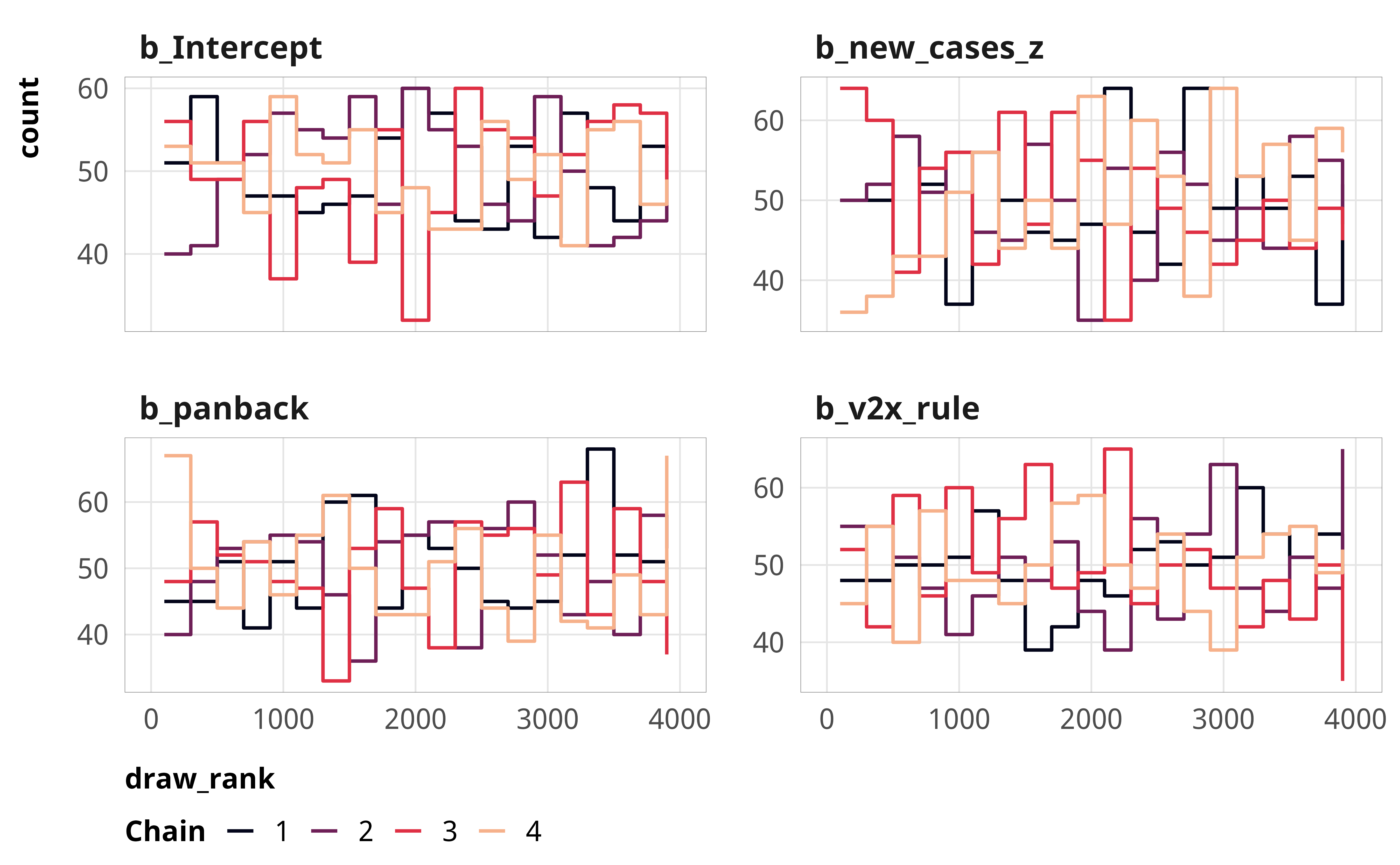
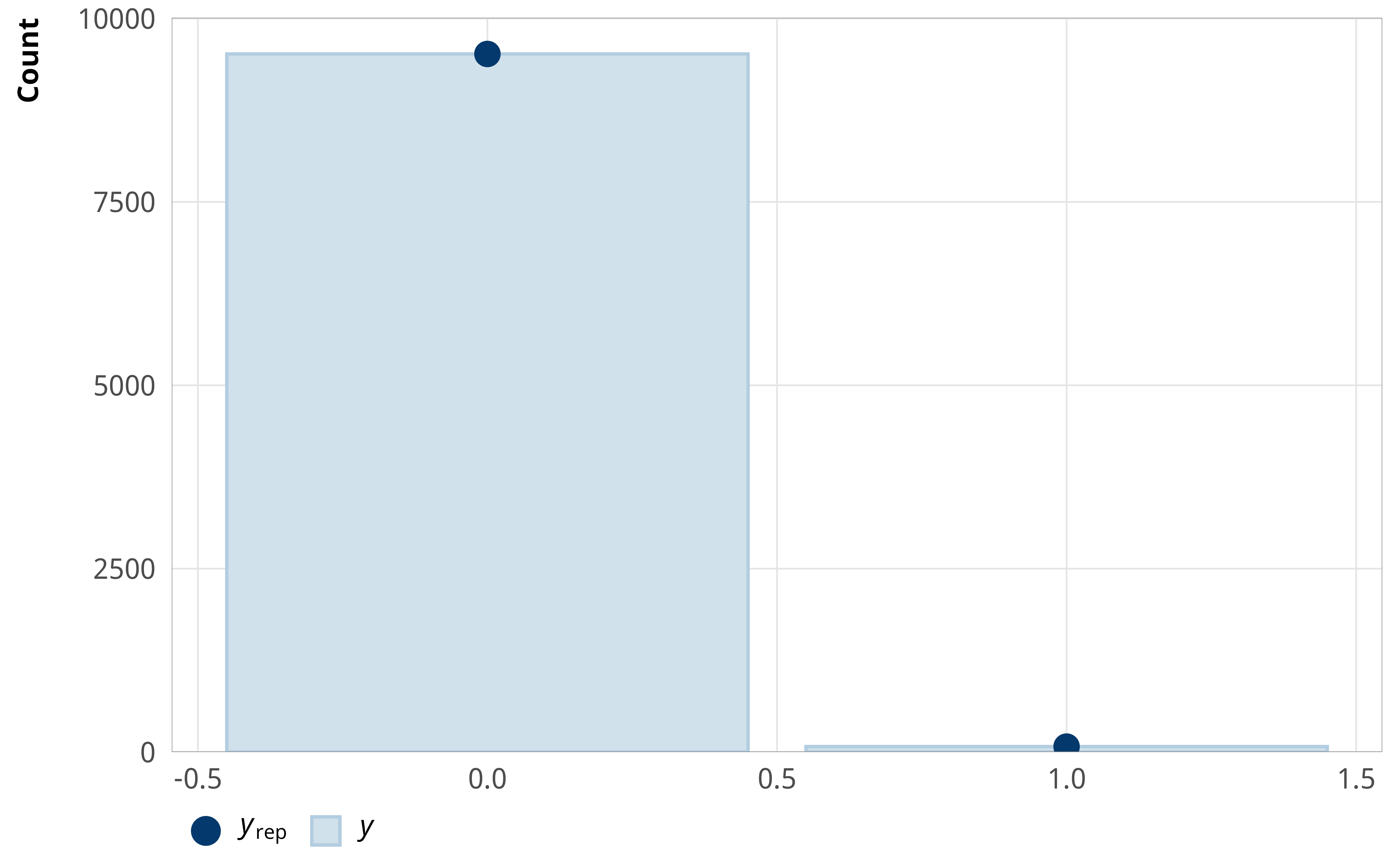
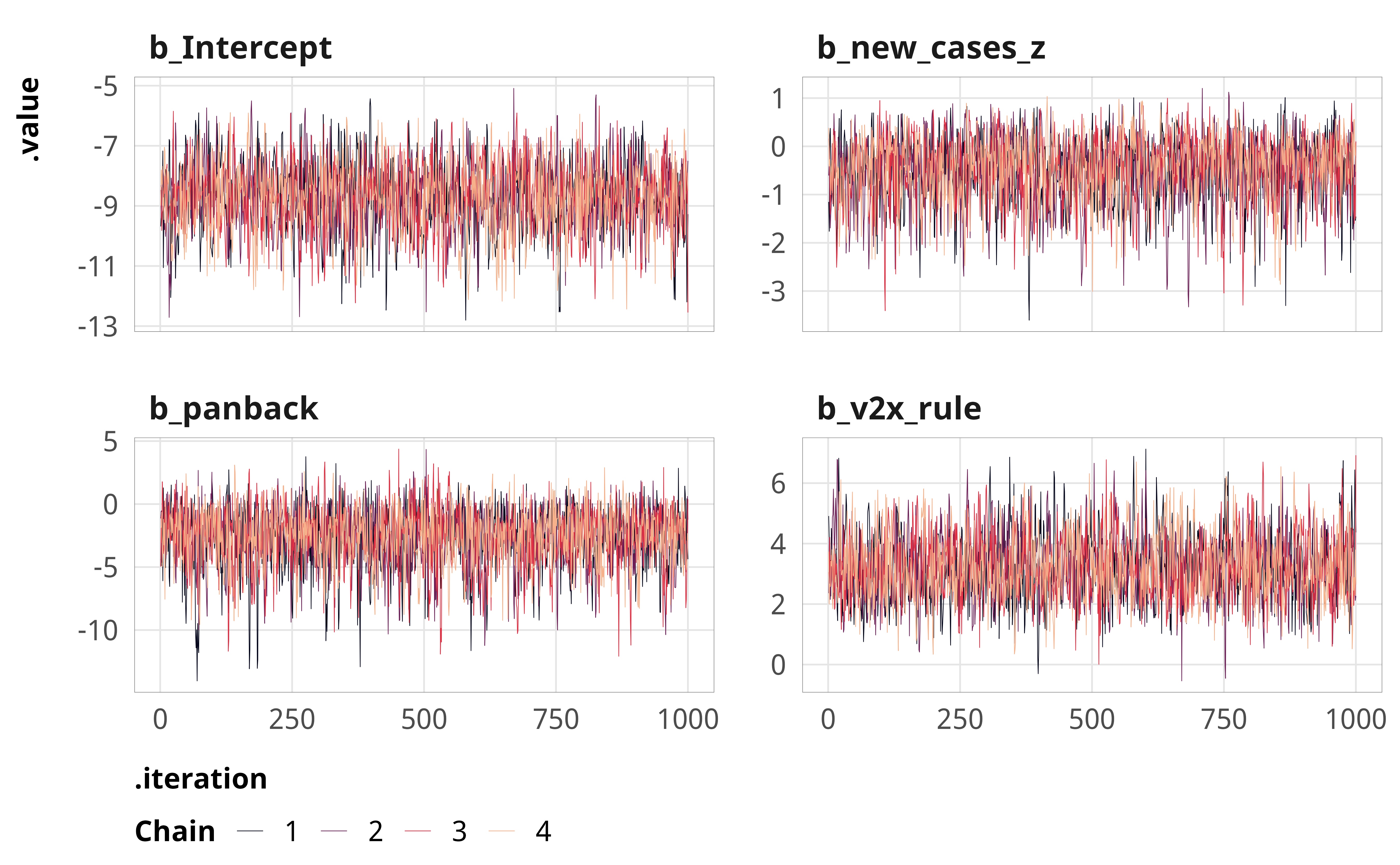
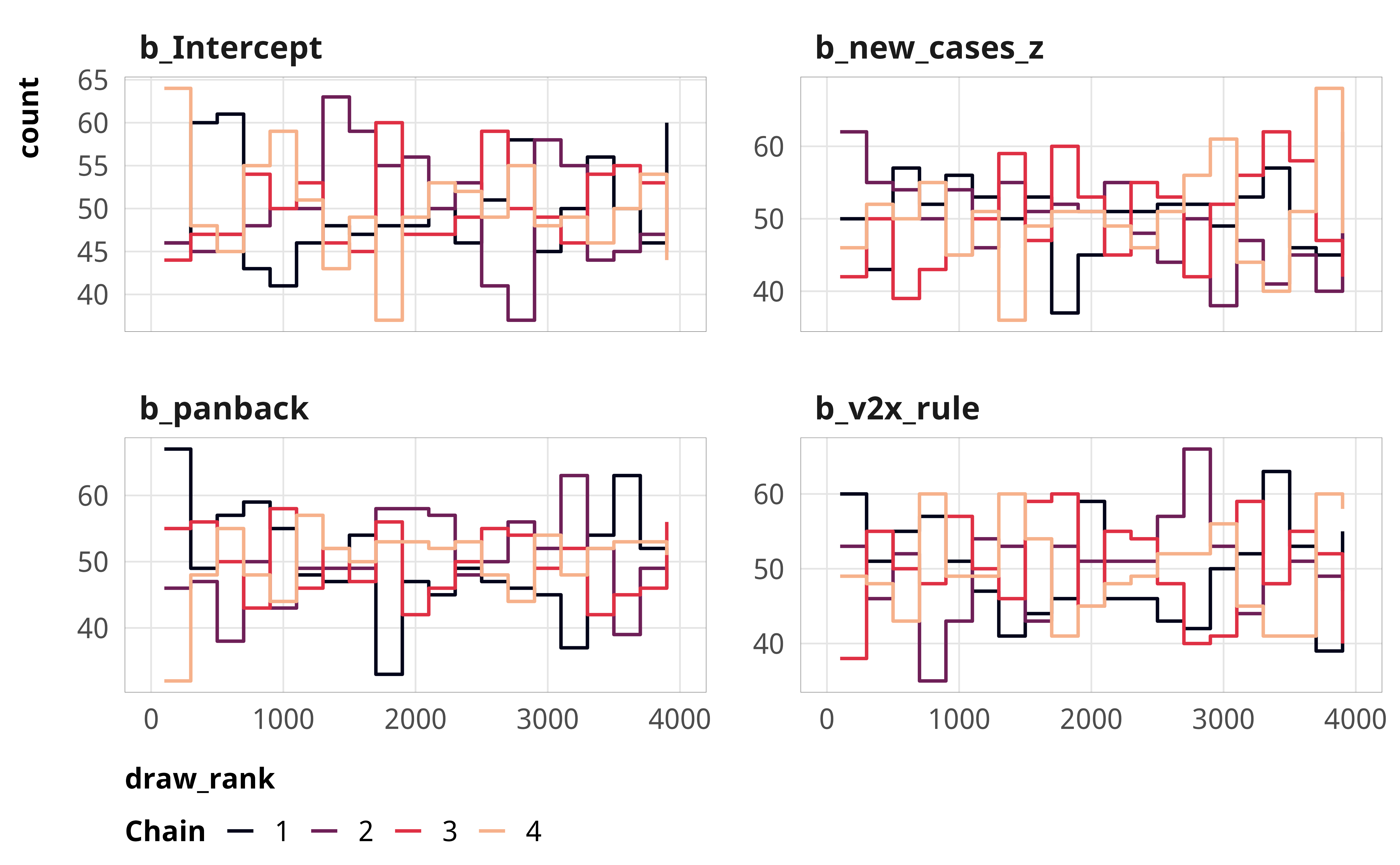
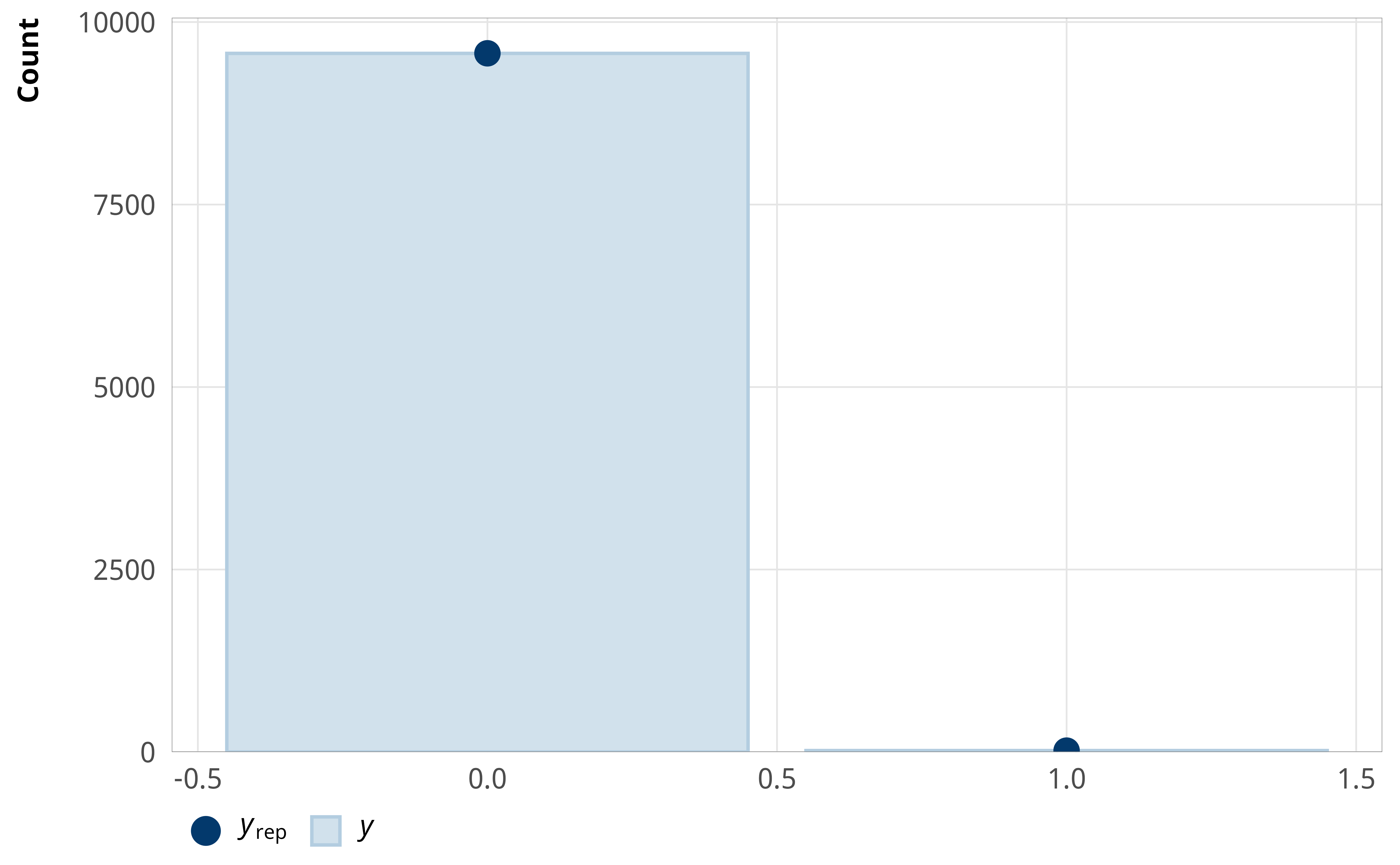
Source Code
---title: "Explaining derogations"format: html: code-fold: true---```{r}#| label: setup#| include: falseknitr::opts_chunk$set(fig.width =6, fig.height = (6*0.618), out.width ="80%",fig.align ="center", fig.retina =3,collapse =TRUE)options(digits =3, width =120, dplyr.summarise.inform =FALSE)``````{r}#| label: libraries-data#| warning: false#| message: falselibrary(tidyverse)library(tidybayes)library(modelsummary)library(scales)library(glue)library(ggtext)library(tinytable)library(targets)tar_config_set(store = here::here("_targets"),script = here::here("_targets.R"))tar_load(c(m_derogations, m_tbl_derogations, action_state_type))invisible(list2env(tar_read(graphic_functions), .GlobalEnv))invisible(list2env(tar_read(diagnostic_functions), .GlobalEnv))invisible(list2env(tar_read(helper_functions), .GlobalEnv))invisible(list2env(tar_read(modelsummary_functions), .GlobalEnv))```# Model details## Formal model specification$$\begin{aligned}&\ \mathrlap{\textbf{Binary outcome $i$ across week $t$}} \\\text{Treaty action}_{it_j} \sim&\ \operatorname{Bernoulli}(\pi_{it_j}) \\[0.75em]&\ \textbf{Distribution parameters} \\\pi_{it} =&\ \beta_0 + \beta_1\ \text{PanBack}_{it} + \\&\ \beta_2\ \text{New cases}_{it}\ + \beta_3\ \text{Cumulative cases}_{it}\ + \\&\ \beta_4\ \text{New deaths}_{it}\ + \beta_5\ \text{Cumulative deaths}_{it}\ + \\&\ \beta_6\ \text{Rule of law index}_{it}\ + \beta_7\ \text{Week number}_{it} \\[0.75em]&\ \textbf{Priors} \\\beta_{0 \dots 7} \sim&\ \operatorname{Student\ t}(\nu = 1, \mu = 0, \sigma = 3)\end{aligned}$$## Priors```{r}#| label: figure-prior#| fig-cap: "Density plot of prior distribution for model parameters"#| fig-width: 3.5#| fig-height: 2.5#| out-width: "50%"ggplot() +stat_function(geom ="area",fun =~extraDistr::dlst(., df =1, mu =0, sigma =3),fill = clrs[2] ) +xlim(c(-20, 20)) +labs(x ="βs") +facet_wrap(vars("β: Student t(ν = 1, µ = 0, σ = 3)")) +theme_pandem(prior =TRUE)```## Simplified R code```rbrm(bf(outcome ~ panback + new_cases_z + cumulative_cases_z + new_deaths_z + cumulative_deaths_z + v2x_rule + year_week_num),family =bernoulli(),prior =c(prior(student_t(1, 0, 3), class = Intercept),prior(student_t(1, 0, 3), class = b)), ...)```## Model evaluation```{r}params_to_show <-c("b_Intercept", "b_panback", "b_new_cases_z", "b_v2x_rule")```::: {.panel-tabset}### Derogation filed```{r}plot_trace(m_derogations$m_derogations_panback, params_to_show)``````{r}plot_trank(m_derogations$m_derogations_panback, params_to_show)``````{r}plot_pp(m_derogations$m_derogations_panback)```### Other treaty action```{r}plot_trace(m_derogations$m_other_panback, params_to_show)``````{r}plot_trank(m_derogations$m_other_panback, params_to_show)``````{r}plot_pp(m_derogations$m_other_panback)```:::# Results```{r}#| label: calc-derog-coefscoef_lookup <-tribble(~coef, ~coef_nice,"b_panback", "Pandemic backsliding index (PanBack)","b_v2x_rule", "Rule of law index","b_new_cases_z", "New cases (standardized)","b_cumulative_cases_z", "Cumulative cases (standardized)","b_new_deaths_z", "New deaths (standardized)","b_cumulative_deaths_z", "Cumulative deaths (standardized)") |>mutate(coef_nice =fct_inorder(coef_nice))m_derog_draws <- m_derogations$m_derogations_panback |>gather_draws(`^b_.*`, regex =TRUE) |>filter(.variable %in% coef_lookup$coef) |>left_join(coef_lookup, by =join_by(.variable == coef))derog_coefs <- m_derog_draws |>mutate(.value_exp =exp(.value)) |>group_by(.variable, coef_nice) |>reframe(post_medians =median_hdci(.value_exp, .width =0.95),p_gt_0 =sum(.value_exp >1) /n() ) |>unnest(post_medians) |>mutate(y_nice =fmt_coef(y),y_nice_html =fmt_coef(y, html =TRUE) ) |>mutate(p_lt_0 =1- p_gt_0,p_gt =fmt_p_inline(p_gt_0, "gt"),p_lt =fmt_p_inline(p_lt_0, "lt"),p_gt_html =fmt_p_inline(p_gt_0, "gt", html =TRUE),p_lt_html =fmt_p_inline(p_lt_0, "lt", html =TRUE) ) |>mutate(p_d =if_else(y >1, p_gt, p_lt),p_d_html =if_else(y >1, p_gt_html, p_lt_html),plot_label =glue("{y_nice_html}; {p_d_html}") ) |>mutate(or_pct =label_percent(accuracy =1)(abs(1- y)))```## Coefficient plot```{r}#| label: figure-derog-coefs#| fig-width: 6#| fig-height: 4.5#| fig-cap: "Odds ratios for coefficients from logistic regression model predicting the probability of derogation from the ICCPR"#| out-width: 100%m_derog_draws |>mutate(.value =exp(.value)) |>ggplot(aes(x = .value, y =fct_rev(coef_nice))) +stat_pointinterval() +geom_vline(xintercept =1, linewidth =0.25, linetype ="21") +geom_richtext(data = derog_coefs, aes(x = y, label = plot_label),size =2.7, nudge_y =0.35, label.size =0.1, label.colour ="grey50" ) +scale_x_log10() +labs(x ="Odds ratio", y =NULL,caption =str_wrap(glue("Point shows posterior median;", " thick lines show 80% credible interval;","thin black lines show 95% credible interval",.sep =" " ),width =60 ) ) +theme_pandem() +theme(panel.grid.major.y =element_blank())```## Complete table of results```{r}#| label: table-results-full-derogations#| tbl-cap: "Complete results from models showing predictors of derogations (H~1~)"notes <-paste("Note: Estimates are median posterior log odds from logistic regression models;","95% credible intervals (highest density posterior interval, or HDPI) in brackets.")m_tbl_derogations |>set_names("Derogation filed", "Other action") |>modelsummary(estimate ="{estimate}",statistic ="[{conf.low}, {conf.high}]",coef_map = coef_map,gof_map = gof_map,output ="tinytable",fmt =fmt_significant(2),notes =c(notes),width =c(0.4, rep(0.3, 2)) ) |>group_tt(j =list("ICCPR action"=2:3)) |>style_tt(j =2:3, align ="c") |>style_tt(i =seq(1, 15, 2), j =1, rowspan =2, alignv ="t") |>style_tt(bootstrap_class ="table table-sm" )```