library(tidyverse)library(targets)library(brms)library(ordbetareg)library(marginaleffects)library(tidybayes)library(ggdist)library(patchwork)library(scales)# Generated via random.orgset.seed(196491)# Load targetstar_load(ongo)tar_load(c(m_full_ordbeta, m_full_zoib))invisible(list2env(tar_read(graphic_functions), .GlobalEnv))theme_set(theme_ongo())
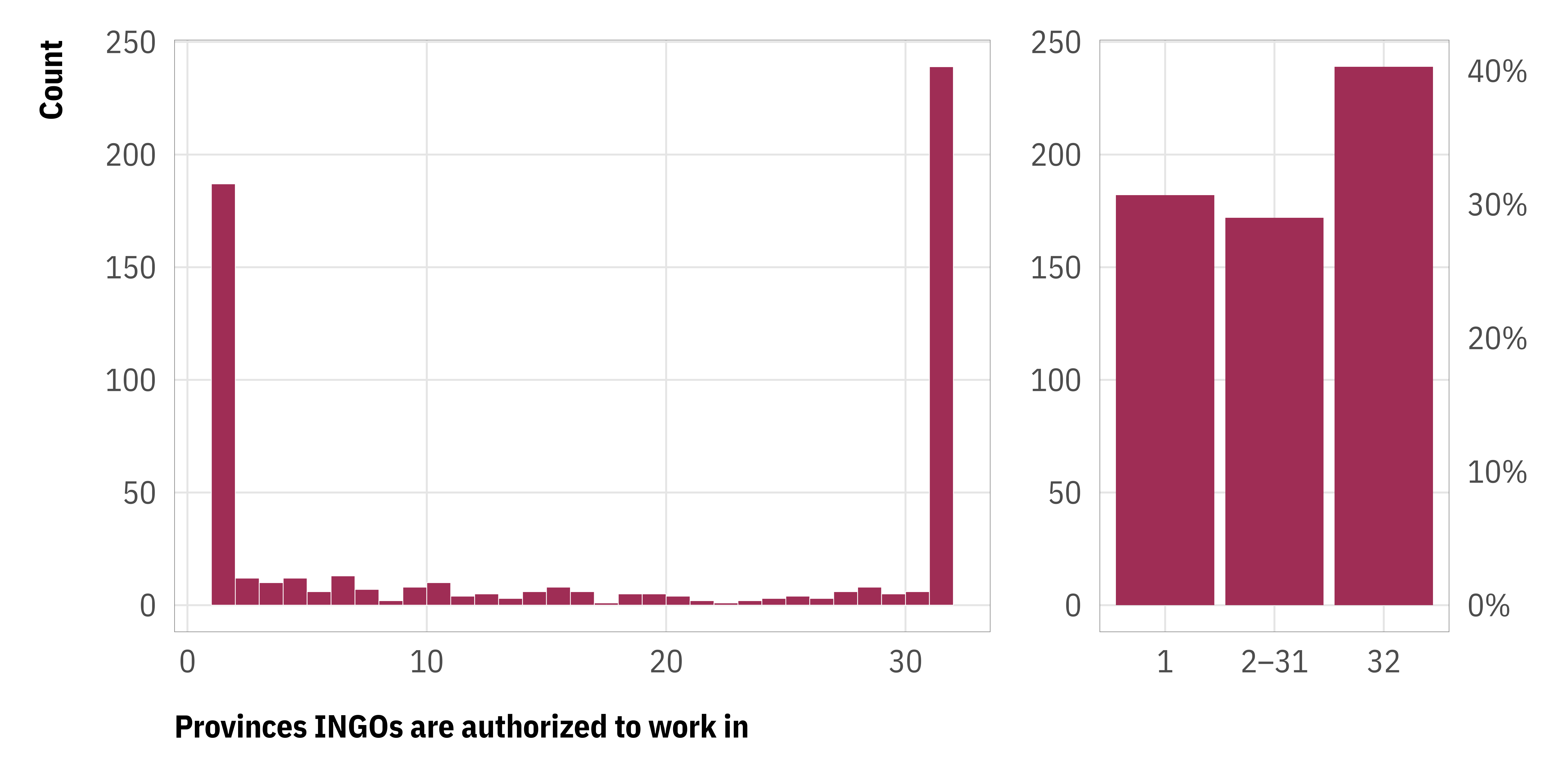
The distribution of our outcome here—the number of provinces an INGO is authorized to work in—poses a unique statistical challenge. It’s a mix of three different processes. 30ish% of INGOs are registered only in one province, 40% are registered in all provinces, and the remaining 30ish% are registered in 2–31 provinces.
Additionally, the outcome is bounded between 1 and 32 and we don’t want predicted values to go beyond those limits. Using something like OLS thus doesn’t work, since (1) it can’t capture all three of the only-one, nationwide, or somewhere-in-between processes, and (2) it just draws straight lines that will create predictions like −5 or 42 provinces.
Proportions instead of counts
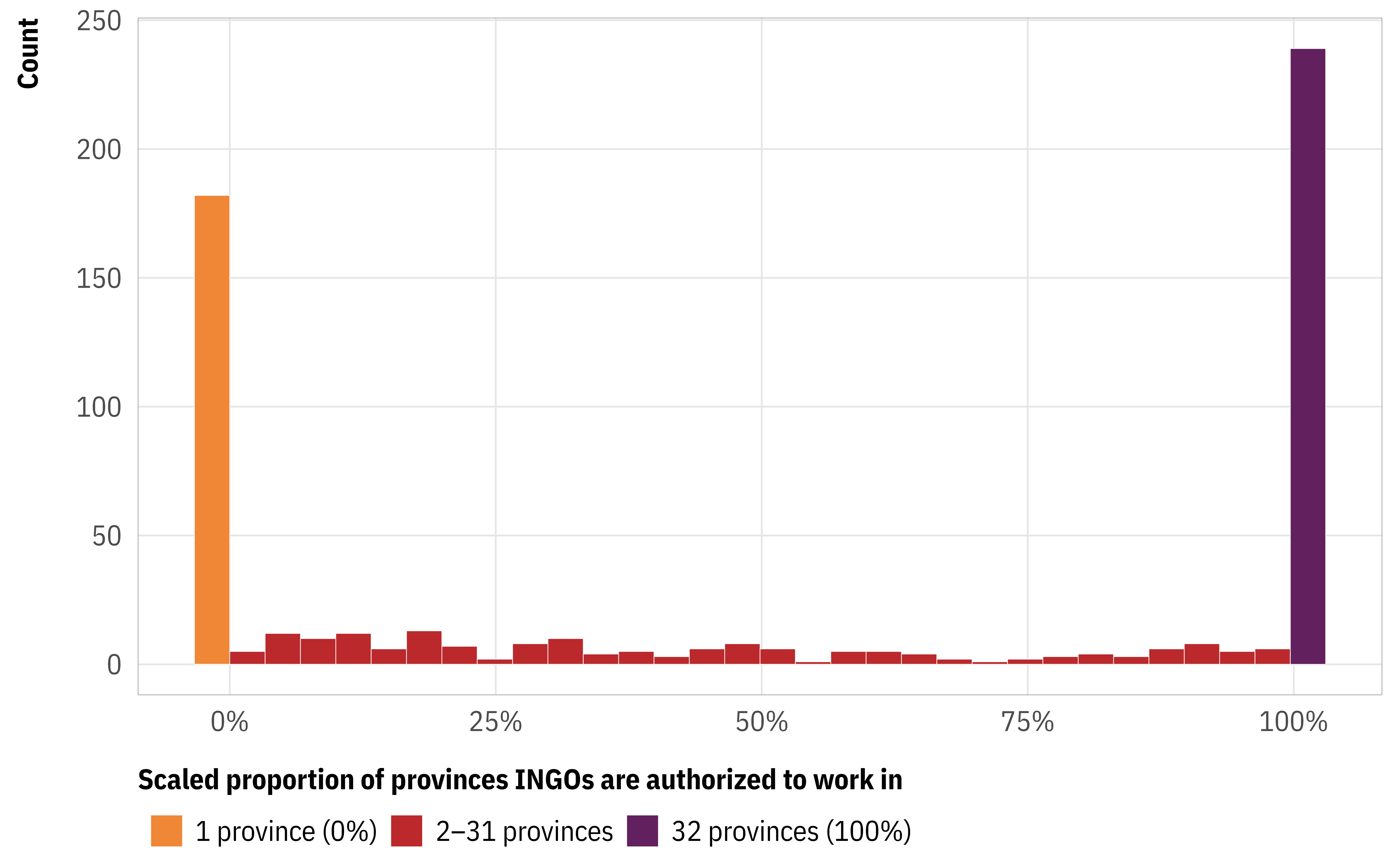
We can constrain predictions of the outcome variable by working with proportions instead of counts, which lets us use Beta regression, which naturally limits outcomes to between 0–1. We can scale the count variable down to a 0–1 range by making 32 provinces = 1, 1 province = 0, and all the in-between province counts some percentage. Just dividing the count by 32 doesn’t quite work—32/32 is indeed 1, but 1/32 is 0.031, not the 0 we’re looking for. Instead, we can subtract 1 from the province count and the total, so that 32 provinces is 31/31, 1 province is 0/31, and so on:
\[
\frac{\text{Province count} - 1}{32 - 1}
\]
We can reverse this process too by multiplying the proportion by 31 and adding 1:
\[
[\text{Province count} \times (32 - 1)] + 1
\]
We can make this easier and more generalizable with some helper functions:
The distribution of proportions is the same as it was for counts, as expected, but now everything is between 0 and 1 and with a lot of values that are exactly 0 or 1:
Code
ongo |>mutate(province_prop =provinces_to_prop(province_count)) |># Add some variables for plottingmutate(is_zero = province_prop ==0,is_one = province_prop ==1,province_prop =case_when( is_zero ~-0.01, is_one ~1.02,.default = province_prop ) ) |>mutate(outcome_type =case_when( is_zero ~"1 province (0%)", is_one ~"32 provinces (100%)",.default ="2–31 provinces" )) |>ggplot(aes(x = province_prop)) +geom_histogram(aes(fill = outcome_type),bins =32, linewidth =0.1, boundary =0,color ="white") +scale_x_continuous(labels =label_percent()) +scale_y_continuous(breaks =seq(0, 250, 50)) +scale_fill_manual(values = clrs[c(3, 5, 7)]) +labs(x ="Scaled proportion of provinces INGOs are authorized to work in", y ="Count", fill =NULL) +theme_ongo()
Zero-one-inflated Beta (ZOIB) regression
Beta regression by itself can’t deal with values that are exactly 0 or 1, but we can use zero-one-inflated beta (ZOIB) regression to deal with them (see this for a guide about that). For zero-one-inflated regression, we actually model three different processes:
A logistic regression model that predicts if an outcome is either (1) exactly 0 or 1 or (2) not exactly 0 or 1. This is typically defined as \(\alpha\), or zoi in {brms}
A logistic regression model that predicts if the exactly-0-or-1 outcomes are either (1) 0 or (2) 1. This is typically defined as \(\gamma\), or coi in {brms}
A Beta regression model that works with the not-exactly-0-or-1 outcomes. These Beta parameters are typically defined as \(\mu\) and \(\phi\), or name_of_outcome and phi in {brms}
This kind of model works really well for our weird {0, (0, 1), 1} outcome, but it requires that we specify covariates for each process of the model. That’s both neat (if we have theoretical reasons that the 0 process is different from the 1 process, for instance, we can use different covariates) and intimidating (SO MANY PARAMETERS).
As an example, here’s what our full model looks like when using zero-one-inflated regression:
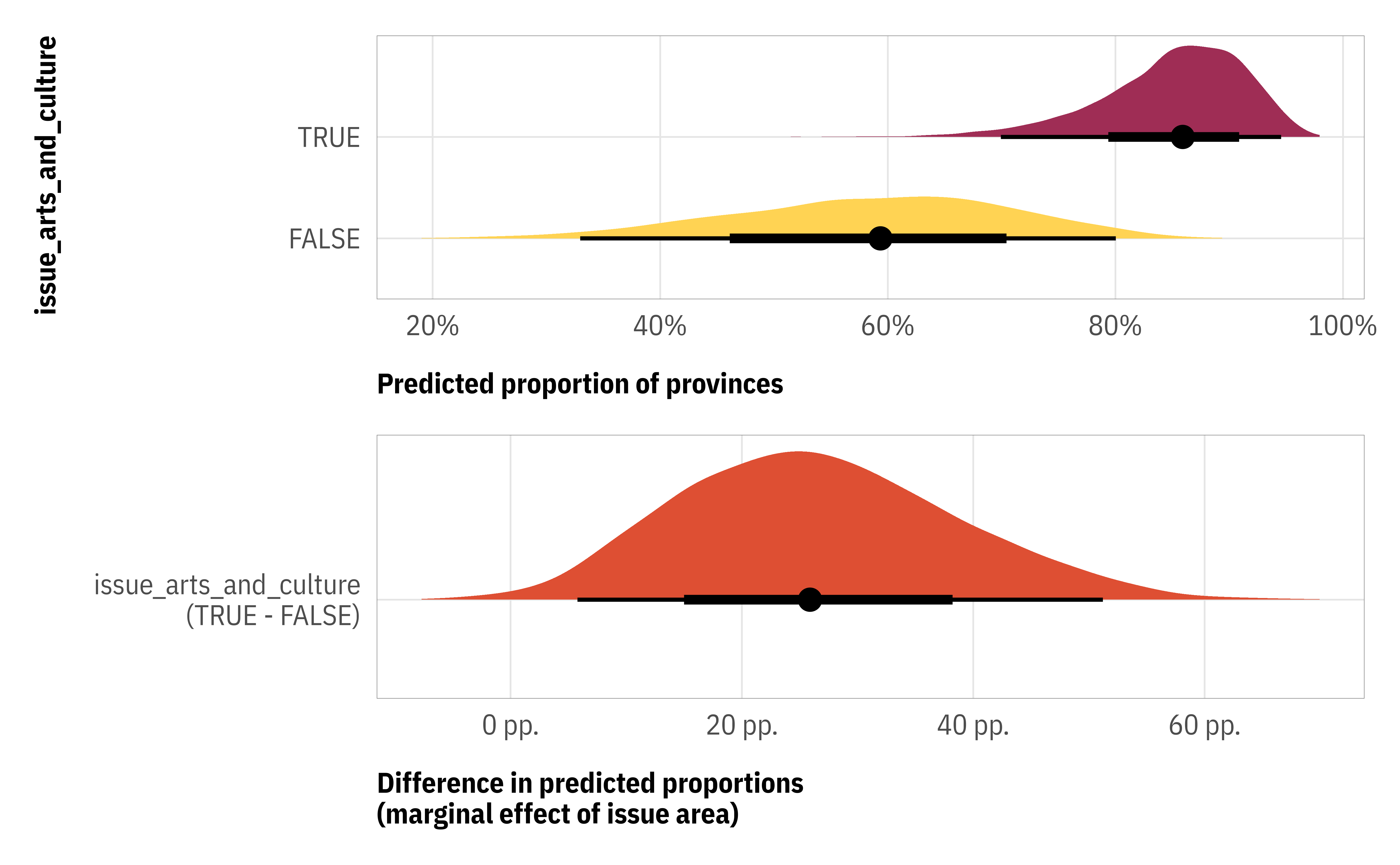
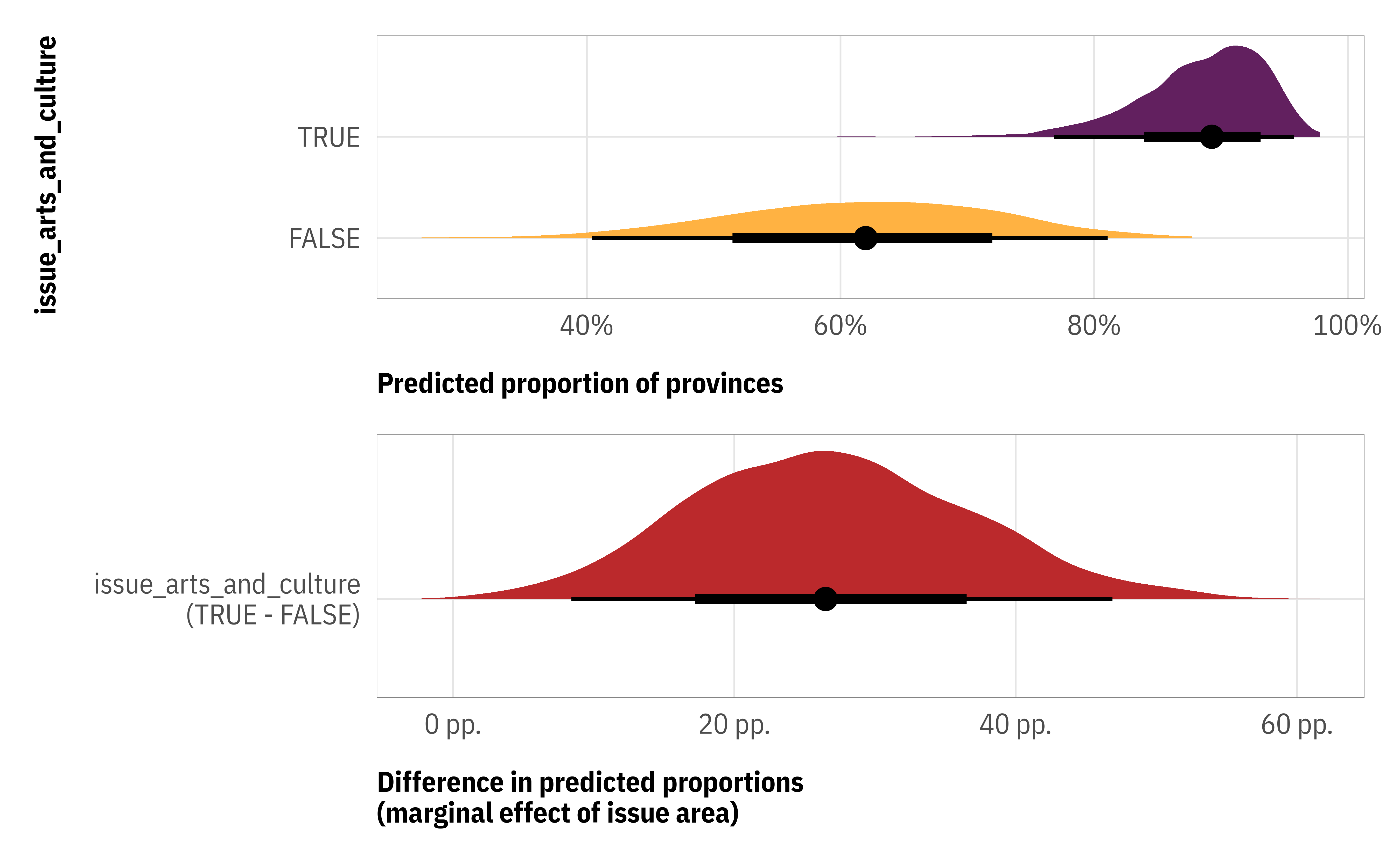
If we’re interested in the effect of one of these coefficients, like issue_arts_and_culture, we need need to work with three different versions of it: issue_arts_and_culture (for the 0-1 process), zoi_issue_arts_and_culture (for the exactly-0-or-1 process), and coi_issue_arts_and_culture (for the 0 or 1 process). To do this, we can calculate predictions that average over (or marginalize over) all three submodels. We can do that with marginaleffects::predictions() and marginaleffects::avg_comparisons():
Zero-one-inflated Beta regression works, but it’s complicated. So instead, we can use a special version of ZOIB regression called “ordered Beta regression” (Kubinec 2022)—see here for a tutorial about it.
To grossly oversimplify how this all works, an ordered Beta model is essentially a zero-one-inflated Beta model fused with an ordinal logistic regression model. With ordered logit, we model the probability of ordered categories (e.g. “strongly disagree”, “disagree”, “neutral”, “agree”, “strongly agree”) with a single set of covariates that predicts cutpoints between each category. That is, each coefficient shows the effect of moving from “strongly disagree” to any of the other options, then (“strongly disagree” or “disagree”) to the other options, and so on, with cutpoint parameters showing the boundaries or thresholds between the probabilities of these categories. Since there’s only one underlying process, there’s only one set of coefficients to work with, which makes post-processing and interpretation fairly straightforward—there’s no need to worry about separate zoi and coi parts!
Ordered Beta models apply the same intuition to Beta regression. Beta regression can’t handle outcomes that are exactly 0 or 1, so we can create three ordered categories to use as an outcome variable: (1) exactly 0, (2) somewhere between 0 and 1, and (3) exactly 1. Then, instead of using logistic regression to model the process of moving along the range of probabilities for these categories (i.e. from “exactly 0” to (“somewhere between 0 and 1” or “exactly 1”) and then from (“exactly 0” or “somewhere between 0 and 1”) to “exactly 1”), we use Beta regression, which captures continuous values between 0-1.
The ordbetareg() function from {ordbetareg} is a wrapper around brm() that handles this hybrid sort of model. It also automatically scales down the data to be a percentage within specific bounds, so we don’t need to model province_pct, and can model province_count directly.
Check out these results. We have just one set of coefficients now (no more zoi and coi), and we have ordered-logit-esque cutpoints for moving between the exactly-0 and exactly-1 categories. It’s Beta regression and ordered regression at the same time. Magic!
These coefficients are on an uninterpretable log odds scale (since it’s a Beta regression model), so we need to use something like {marginaleffects} or posterior_epred() to get these into useful proportion scale estimates:
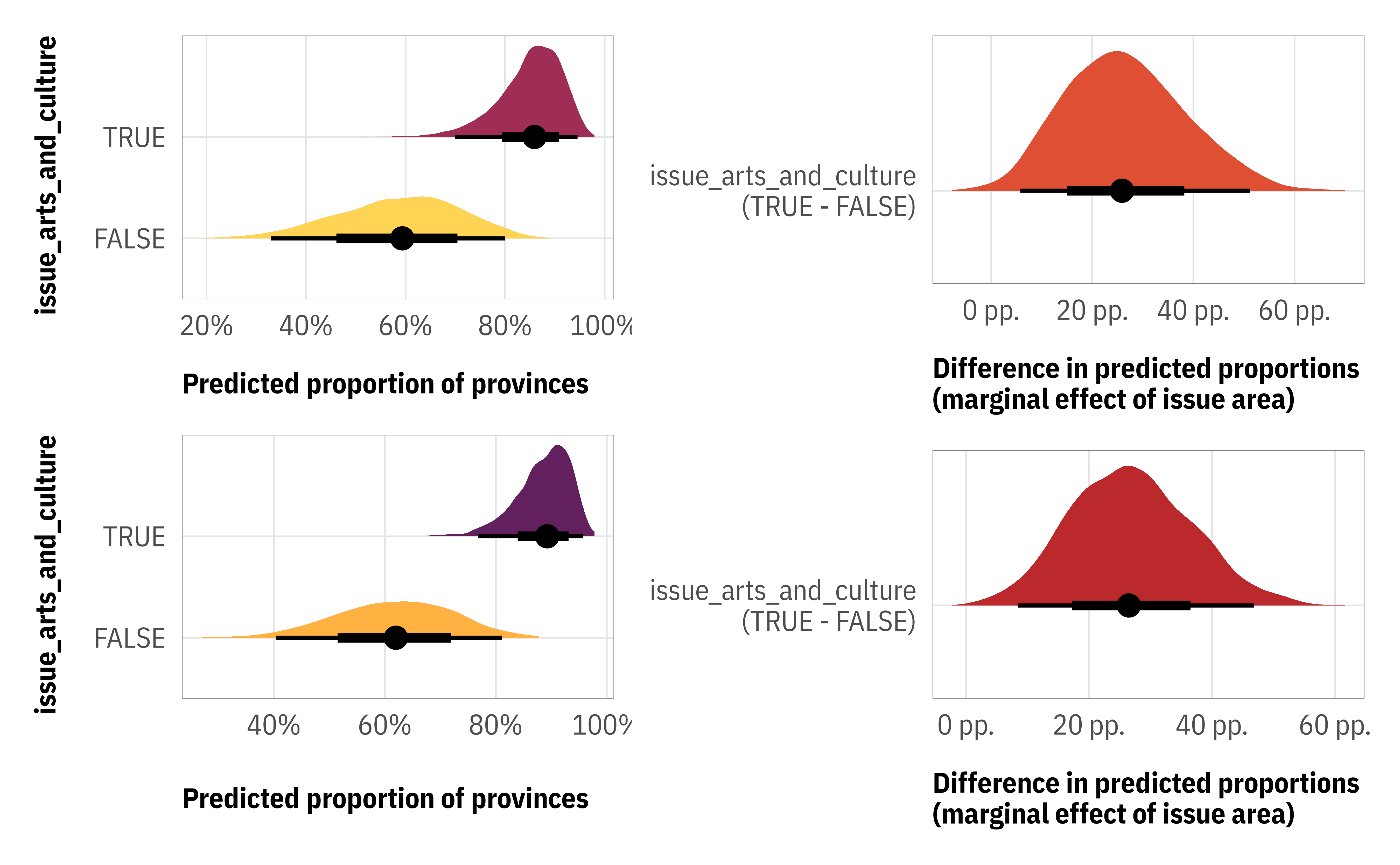
The estimates are roughly comparable to the zero-one-inflated model, though Kubinec (2022) shows that the ordered Beta results are generally more accurate and less biased. Plus this model fit a ton faster since we didn’t need to specify complete separate models for the zoi and coi processes.
Code
(p1 / p3) | (p2 / p4)
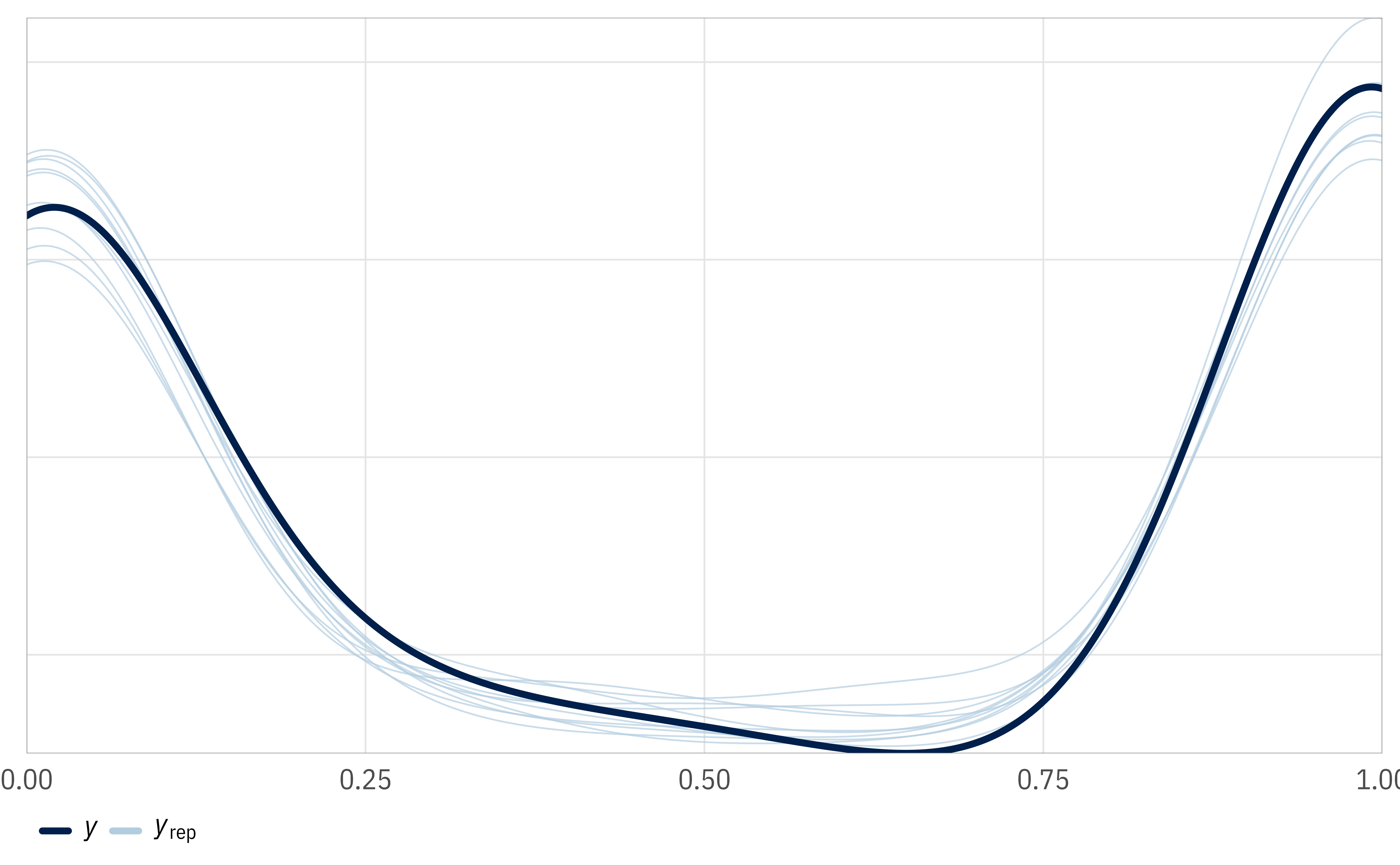
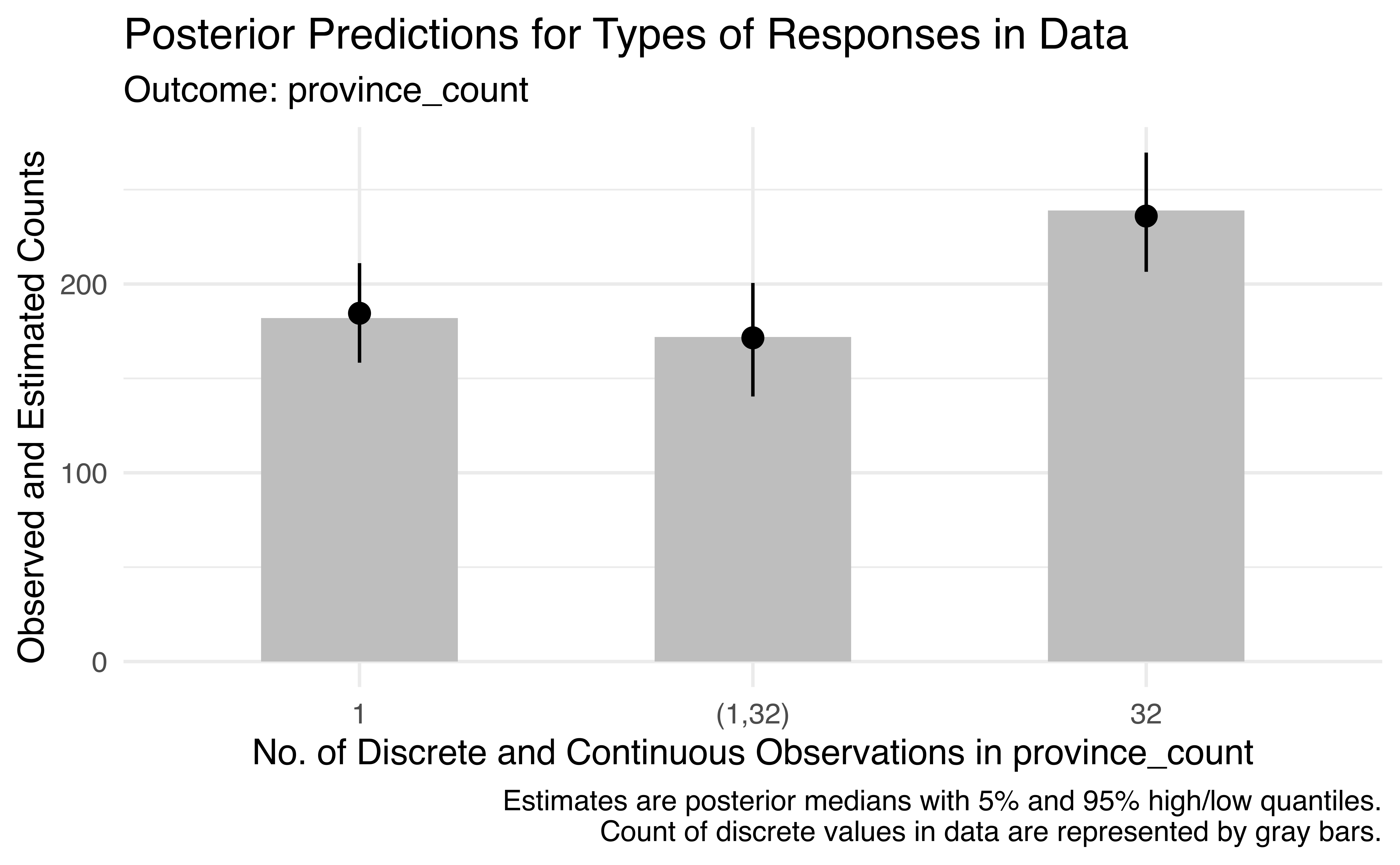
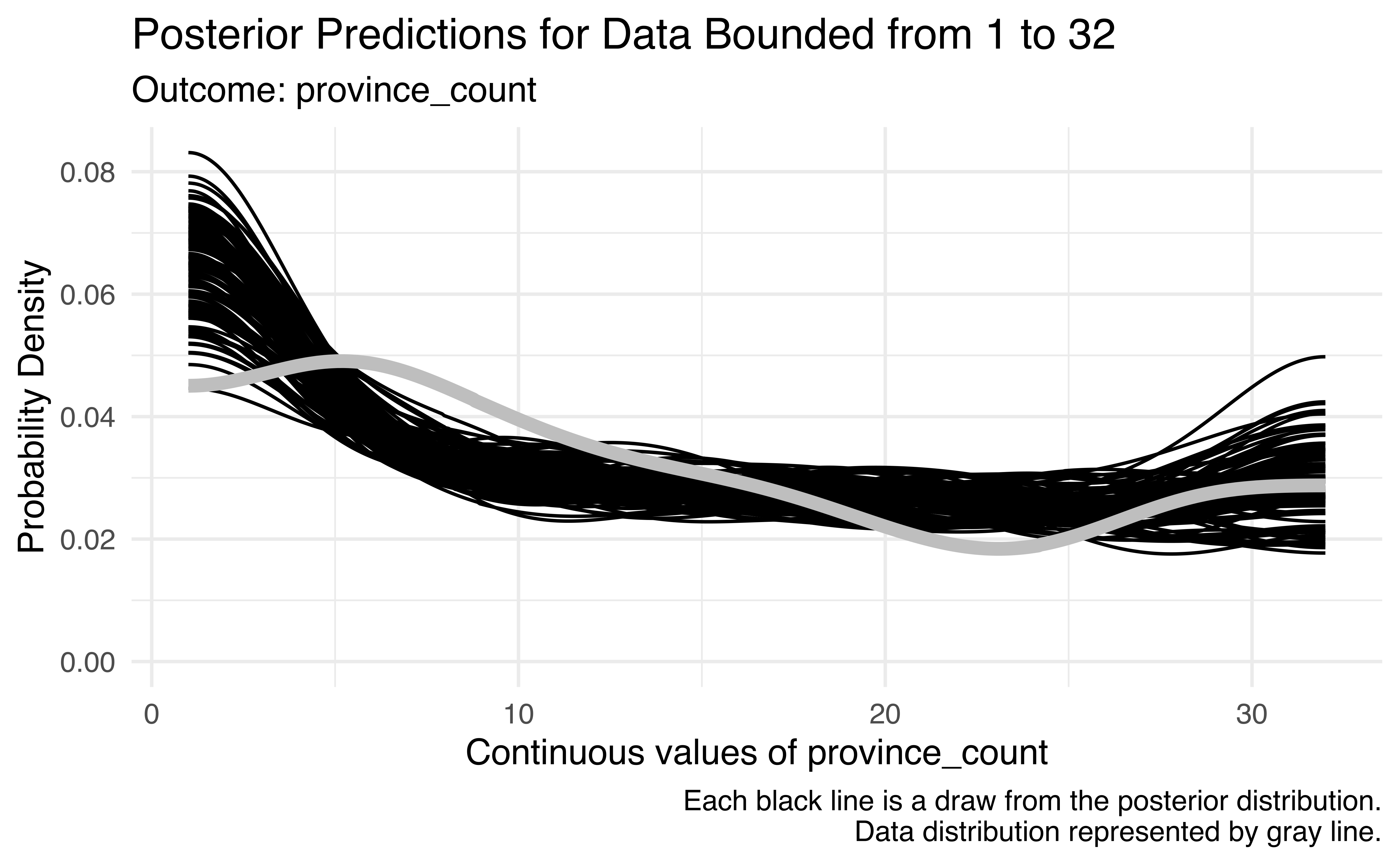
The posterior predictions are also pretty neat and different. The standard pp_check() function doesn’t work because the model generates both categorical and continuous predictions, so {ordbetareg} comes with its own pp_check_ordbeta() that contains plots in slots named $discrete and $continuous. It automatically converts the proportion/probability-scale predicted outcomes back into discrete counts, so instead of seeing predictions that range from 0% to 100%, we get predictions for exactly 1, exactly 32, and between 1 and 32 provinces. Neat! (See here for a fancier, more manual version of these plots.)
Kubinec, Robert. 2022. “Ordered Beta Regression: A Parsimonious, Well-Fitting Model for Continuous Data with Lower and Upper Bounds.”Political Analysis, 1–18. https://doi.org/10.31235/osf.io/2sx6y.
Source Code
---title: "Why ordered beta regression"---```{r setup, include=FALSE}knitr::opts_chunk$set(fig.align = "center", fig.retina = 3, fig.width = 6, fig.height = (6 * 0.618), out.width = "80%", collapse = TRUE, dev = "png", dev.args = list(type = "cairo-png"))options(digits = 3, width = 120, dplyr.summarise.inform = FALSE, knitr.kable.NA = "")``````{r load-libraries, warning=FALSE, message=FALSE}library(tidyverse)library(targets)library(brms)library(ordbetareg)library(marginaleffects)library(tidybayes)library(ggdist)library(patchwork)library(scales)# Generated via random.orgset.seed(196491)# Load targetstar_load(ongo)tar_load(c(m_full_ordbeta, m_full_zoib))invisible(list2env(tar_read(graphic_functions), .GlobalEnv))theme_set(theme_ongo())```The distribution of our outcome here—the number of provinces an INGO is authorized to work in—poses a unique statistical challenge. It's a mix of three different processes. 30ish% of INGOs are registered only in one province, 40% are registered in all provinces, and the remaining 30ish% are registered in 2–31 provinces.```{r plot-province-count-collapsed, fig.width=6, fig.height=3}provinces_collapsed <- ongo |> drop_na(province_count) |> mutate(province_count = case_when( province_count == 1 ~ "1", province_count > 1 & province_count < 32 ~ "2–31", province_count == 32 ~ "32" ))p1 <- ggplot(ongo, aes(x = province_count)) + geom_histogram(binwidth = 1, linewidth = 0.1, boundary = 0, fill = clrs[6], color = "white") + scale_y_continuous(breaks = seq(0, 250, 50)) + labs(x = "Provinces INGOs are authorized to work in", y = "Count") + theme_ongo()p2 <- ggplot(provinces_collapsed, aes(x = province_count)) + geom_bar(fill = clrs[6]) + scale_x_discrete(labels = label_wrap(10)) + scale_y_continuous(sec.axis = sec_axis(trans = ~ . / nrow(provinces_collapsed), labels = label_percent()), breaks = seq(0, 250, 50)) + labs(x = NULL, y = NULL) + theme_ongo()(p1 | p2) + plot_layout(nrow = 1, widths = c(0.7, 0.3))```Additionally, the outcome is bounded between 1 and 32 and we don't want predicted values to go beyond those limits. Using something like OLS thus doesn't work, since (1) it can't capture all three of the only-one, nationwide, or somewhere-in-between processes, and (2) it just draws straight lines that will create predictions like −5 or 42 provinces.# Proportions instead of countsWe can constrain predictions of the outcome variable by working with proportions instead of counts, which lets us use Beta regression, which naturally limits outcomes to between 0–1. We can scale the count variable down to a 0–1 range by making 32 provinces = 1, 1 province = 0, and all the in-between province counts some percentage. Just dividing the count by 32 doesn't quite work—32/32 is indeed 1, but 1/32 is `r 1/32`, not the 0 we're looking for. Instead, we can subtract 1 from the province count and the total, so that 32 provinces is 31/31, 1 province is 0/31, and so on:$$\frac{\text{Province count} - 1}{32 - 1}$$We can reverse this process too by multiplying the proportion by 31 and adding 1:$$[\text{Province count} \times (32 - 1)] + 1$$We can make this easier and more generalizable with some helper functions:```{r helper-functions}#| code-fold: showprovinces_to_prop <- function(x, lower = 1, upper = 32) { (x - lower) / (upper - lower)}prop_to_provinces <- function(x, lower = 1, upper = 32) { (x * (upper - lower)) + lower}provinces_to_prop(c(1, 5, 19, 32))prop_to_provinces(provinces_to_prop(c(1, 5, 19, 32)))```The distribution of proportions is the same as it was for counts, as expected, but now everything is between 0 and 1 and with a lot of values that are exactly 0 or 1:```{r plot-province-prop}ongo |> mutate(province_prop = provinces_to_prop(province_count)) |> # Add some variables for plotting mutate( is_zero = province_prop == 0, is_one = province_prop == 1, province_prop = case_when( is_zero ~ -0.01, is_one ~ 1.02, .default = province_prop ) ) |> mutate(outcome_type = case_when( is_zero ~ "1 province (0%)", is_one ~ "32 provinces (100%)", .default = "2–31 provinces" )) |> ggplot(aes(x = province_prop)) + geom_histogram( aes(fill = outcome_type), bins = 32, linewidth = 0.1, boundary = 0, color = "white") + scale_x_continuous(labels = label_percent()) + scale_y_continuous(breaks = seq(0, 250, 50)) + scale_fill_manual(values = clrs[c(3, 5, 7)]) + labs( x = "Scaled proportion of provinces INGOs are authorized to work in", y = "Count", fill = NULL) + theme_ongo()```# Zero-one-inflated Beta (ZOIB) regressionBeta regression by itself can't deal with values that are exactly 0 or 1, but we can use zero-one-inflated beta (ZOIB) regression to deal with them ([see this for a guide about that](https://www.andrewheiss.com/blog/2021/11/08/beta-regression-guide/)). For zero-one-inflated regression, we actually model three different processes:1. A logistic regression model that predicts if an outcome is either (1) exactly 0 or 1 or (2) not exactly 0 or 1. This is typically defined as $\alpha$, or `zoi` in {brms}2. A logistic regression model that predicts if the exactly-0-or-1 outcomes are either (1) 0 or (2) 1. This is typically defined as $\gamma$, or `coi` in {brms}3. A Beta regression model that works with the not-exactly-0-or-1 outcomes. These Beta parameters are typically defined as $\mu$ and $\phi$, or `name_of_outcome` and `phi` in {brms}This kind of model works really well for our weird {0, (0, 1), 1} outcome, but it requires that we specify covariates for each process of the model. That's both neat (if we have theoretical reasons that the 0 process is different from the 1 process, for instance, we can use different covariates) and intimidating (SO MANY PARAMETERS). As an example, here's what our full model looks like when using zero-one-inflated regression:```{r model-zoib-example, eval=FALSE}#| code-fold: showm_full_zoib <- brm( bf( # mu: mean of the 0-1 values; logit scale province_pct ~ issue_arts_and_culture + issue_education + issue_industry_association + issue_economy_and_trade + issue_charity_and_humanitarian + issue_general + issue_health + issue_environment + issue_science_and_technology + local_connect + years_since_law + year_registered_cat, # zoi: zero-or-one-inflated part; logit scale zoi ~ issue_arts_and_culture + issue_education + issue_industry_association + issue_economy_and_trade + issue_charity_and_humanitarian + issue_general + issue_health + issue_environment + issue_science_and_technology + local_connect + years_since_law + year_registered_cat, # coi: one-inflated part, conditional on the 0s; logit scale coi ~ issue_arts_and_culture + issue_education + issue_industry_association + issue_economy_and_trade + issue_charity_and_humanitarian + issue_general + issue_health + issue_environment + issue_science_and_technology + local_connect + years_since_law + year_registered_cat), data = data, family = zero_one_inflated_beta(), ...)```The model fits the outcome really well!```{r show-zoib-pp_check, message=FALSE}pp_check(m_full_zoib)```But holy cow it's a huge model. Check out how many different parameters it spits out:```{r show-zoib-summary}#| code-fold: showm_full_zoib```If we're interested in the effect of one of these coefficients, like `issue_arts_and_culture`, we need need to work with three different versions of it: `issue_arts_and_culture` (for the 0-1 process), `zoi_issue_arts_and_culture` (for the exactly-0-or-1 process), and `coi_issue_arts_and_culture` (for the 0 or 1 process). To do this, we can calculate predictions that average over (or marginalize over) all three submodels. We can do that with `marginaleffects::predictions()` and `marginaleffects::avg_comparisons()`:```{r mfx-zoib}p1 <- m_full_zoib |> predictions(datagrid(issue_arts_and_culture = unique)) |> posterior_draws() |> ggplot(aes(x = draw, y = issue_arts_and_culture, fill = issue_arts_and_culture)) + stat_halfeye() + scale_fill_manual(values = clrs[c(1, 6)]) + scale_x_continuous(labels = label_percent()) + guides(fill = "none") + labs(x = "Predicted proportion of provinces")p2 <- m_full_zoib |> avg_comparisons( datagrid(issue_arts_and_culture = unique), variables = "issue_arts_and_culture" ) |> posterior_draws() |> mutate(term_nice = paste0(term, "\n(", contrast, ")")) |> ggplot(aes(x = draw, y = term_nice)) + stat_halfeye(fill = clrs[4]) + scale_x_continuous(labels = label_number(accuracy = 1, scale = 100, suffix = " pp.")) + guides(fill = "none") + labs(x = "Difference in predicted proportions\n(marginal effect of issue area)", y = NULL)p1 / p2```# Ordered Beta regressionZero-one-inflated Beta regression works, but it's complicated. So instead, we can use a special version of ZOIB regression called "ordered Beta regression" [@Kubinec:2022]—[see here for a tutorial about it](https://www.robertkubinec.com/post/limited_dvs/). To *grossly* oversimplify how this all works, an ordered Beta model is essentially a zero-one-inflated Beta model fused with an ordinal logistic regression model. With ordered logit, we model the probability of ordered categories (e.g. "strongly disagree", "disagree", "neutral", "agree", "strongly agree") with a single set of covariates that predicts cutpoints between each category. That is, each coefficient shows the effect of moving from "strongly disagree" to any of the other options, then ("strongly disagree" or "disagree") to the other options, and so on, with cutpoint parameters showing the boundaries or thresholds between the probabilities of these categories. Since there's only one underlying process, there's only one set of coefficients to work with, which makes post-processing and interpretation fairly straightforward—there's no need to worry about separate `zoi` and `coi` parts!Ordered Beta models apply the same intuition to Beta regression. Beta regression can't handle outcomes that are exactly 0 or 1, so we can create three ordered categories to use as an outcome variable: (1) exactly 0, (2) somewhere between 0 and 1, and (3) exactly 1. Then, instead of using logistic regression to model the process of moving along the range of probabilities for these categories (i.e. from "exactly 0" to ("somewhere between 0 and 1" or "exactly 1") and then from ("exactly 0" or "somewhere between 0 and 1") to "exactly 1"), we use Beta regression, which captures continuous values between 0-1.The `ordbetareg()` function from {ordbetareg} is a wrapper around `brm()` that handles this hybrid sort of model. It also automatically scales down the data to be a percentage within specific bounds, so we don't need to model `province_pct`, and can model `province_count` directly.```{r model-ordbeta-example, eval=FALSE}#| code-fold: showm_full_ordbeta <- ordbetareg( bf( province_count ~ issue_arts_and_culture + issue_education + issue_industry_association + issue_economy_and_trade + issue_charity_and_humanitarian + issue_general + issue_health + issue_environment + issue_science_and_technology + local_connect + years_since_law + year_registered_cat ), data = data, true_bounds = c(1, 32), ...)```Check out these results. We have just one set of coefficients now (no more `zoi` and `coi`), and we have ordered-logit-esque cutpoints for moving between the exactly-0 and exactly-1 categories. It's Beta regression *and* ordered regression at the same time. Magic! ```{r show-ordbeta-summary}#| code-fold: showm_full_ordbeta```These coefficients are on an uninterpretable log odds scale (since it's a Beta regression model), so we need to use something like {marginaleffects} or `posterior_epred()` to get these into useful proportion scale estimates:```{r mfx-ordbeta}p3 <- m_full_ordbeta |> predictions(datagrid(issue_arts_and_culture = unique)) |> posterior_draws() |> ggplot(aes(x = draw, y = issue_arts_and_culture, fill = issue_arts_and_culture)) + stat_halfeye() + scale_fill_manual(values = clrs[c(2, 7)]) + scale_x_continuous(labels = label_percent()) + guides(fill = "none") + labs(x = "Predicted proportion of provinces")p4 <- m_full_ordbeta |> avg_comparisons( datagrid(issue_arts_and_culture = unique), variables = "issue_arts_and_culture" ) |> posterior_draws() |> mutate(term_nice = paste0(term, "\n(", contrast, ")")) |> ggplot(aes(x = draw, y = term_nice)) + stat_halfeye(fill = clrs[5]) + scale_x_continuous(labels = label_number(accuracy = 1, scale = 100, suffix = " pp.")) + guides(fill = "none") + labs(x = "Difference in predicted proportions\n(marginal effect of issue area)", y = NULL)p3 / p4```The estimates are roughly comparable to the zero-one-inflated model, though @Kubinec:2022 shows that the ordered Beta results are generally more accurate and less biased. Plus this model fit a ton faster since we didn't need to specify complete separate models for the `zoi` and `coi` processes.```{r compare-mfx}(p1 / p3) | (p2 / p4)```The posterior predictions are also pretty neat and different. The standard `pp_check()` function doesn't work because the model generates both categorical and continuous predictions, so {ordbetareg} comes with its own `pp_check_ordbeta()` that contains plots in slots named `$discrete` and `$continuous`. It automatically converts the proportion/probability-scale predicted outcomes back into discrete counts, so instead of seeing predictions that range from 0% to 100%, we get predictions for exactly 1, exactly 32, and between 1 and 32 provinces. Neat! ([See here for a fancier, more manual version of these plots.](/notebook/model-diagnostics.qmd#posterior-predictions))```{r show-ordbeta-pp_check}#| code-fold: showposterior_check <- pp_check_ordbeta(m_full_ordbeta, ndraws = 100)posterior_check$discreteposterior_check$continuous```