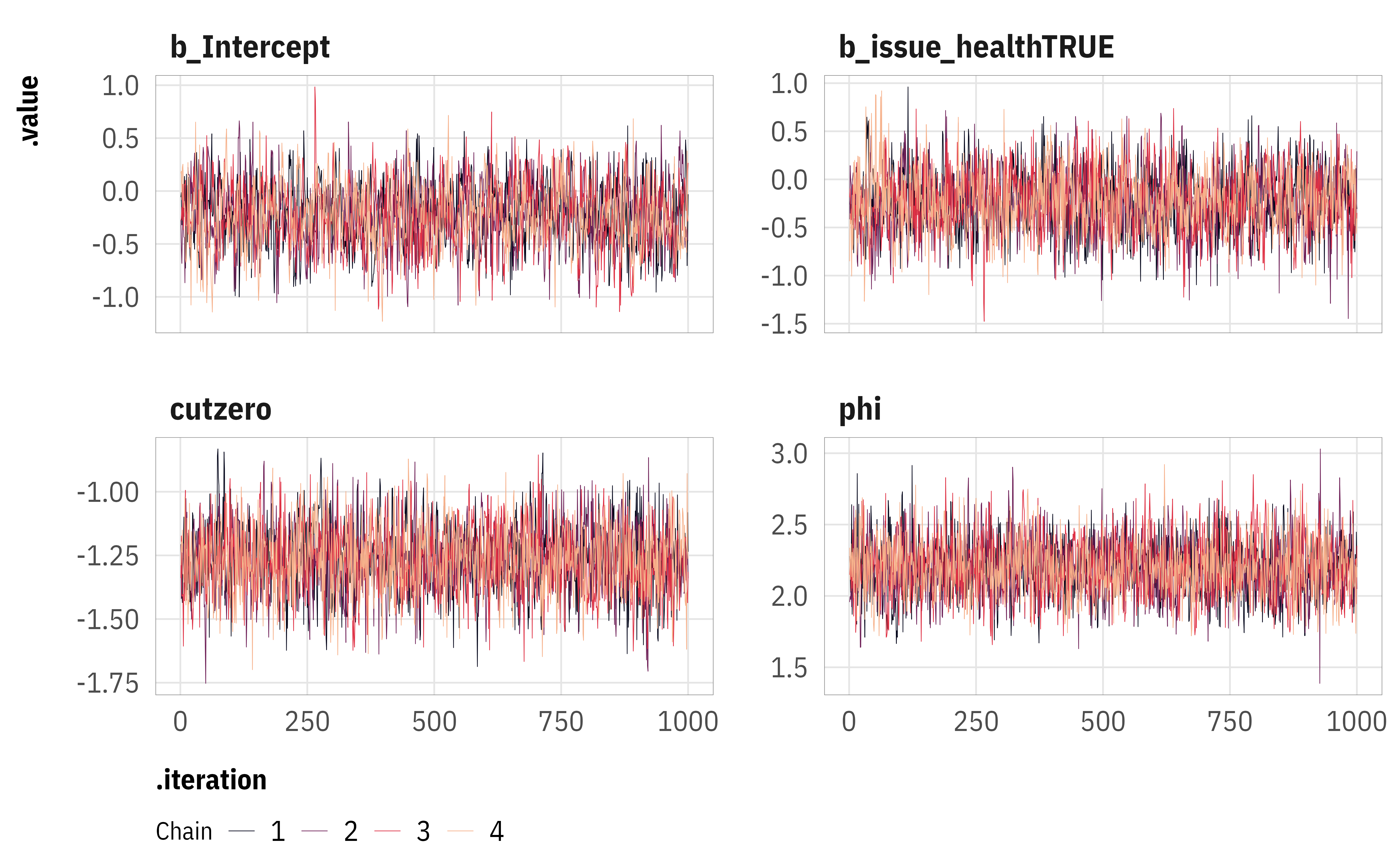
Code
library(tidyverse)
library(targets)
library(tidybayes)
library(glue)
library(patchwork)
library(gt)
library(gtExtras)

tar_config_set(
  store = here::here("_targets"),
  script = here::here("_targets.R")
)

tar_load(m_full_ordbeta)

invisible(list2env(tar_read(graphic_functions), .GlobalEnv))
invisible(list2env(tar_read(table_functions), .GlobalEnv))

theme_set(theme_ongo())

Traceplots

These should look like hairy caterpillars.

They do.

Code
params_to_show <- c(
  "b_Intercept", "b_issue_healthTRUE",
  "phi", "cutzero"
)

m_full_ordbeta |> 
  tidybayes::gather_draws(!!!syms(params_to_show)) |> 
  ggplot(aes(x = .iteration, y = .value, color = factor(.chain))) +
  geom_line(linewidth = 0.1) +
  scale_color_viridis_d(option = "rocket", end = 0.85) +
  labs(color = "Chain") +
  facet_wrap(vars(.variable), scales = "free_y")

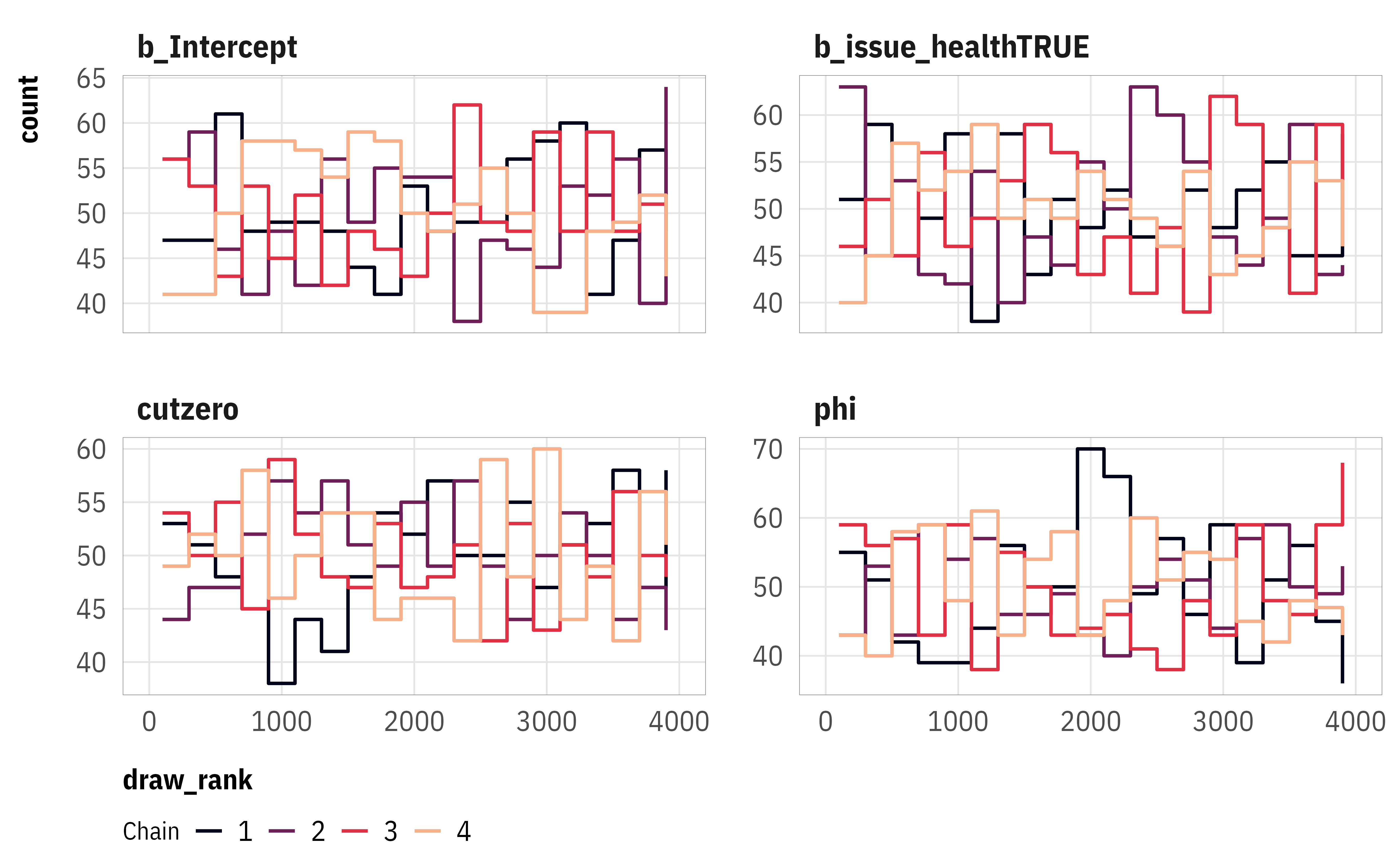
Trace rank plots (trank plots)

These are histograms of the ranks of the parameter draws across the four chains. If the chains are exploring the same space efficiently, the histograms should be similar and overlapping and no one chain should have a specific rank for a long time (McElreath 2020, 284).

They do.

Code
m_full_ordbeta |> 
  tidybayes::gather_draws(!!!syms(params_to_show)) |> 
  group_by(.variable) |> 
  mutate(draw_rank = rank(.value)) |> 
  ggplot(aes(x = draw_rank, color = factor(.chain))) +
  stat_bin(geom = "step", binwidth = 200, position = position_identity(), boundary = 0) +
  scale_color_viridis_d(option = "rocket", end = 0.85) +
  labs(color = "Chain") +
  facet_wrap(vars(.variable), scales = "free_y")

Posterior predictions

The model should generate predictions that align with the observed outcomes. It does.

Code
full_posterior <- predicted_draws(m_full_ordbeta, 
                                  newdata = m_full_ordbeta$data, 
                                  ndraws = 100)

posterior_categories <- full_posterior |> 
  ungroup() |> 
  mutate(outcome = case_when(
    .prediction == 0 ~ "Only 1 province",
    .prediction > 0 & .prediction < 1 ~ "Between 1–32 provinces",
    .prediction == 1 ~ "All 32 provinces",
    .ptype = factor(
      levels = c("Only 1 province", "Between 1–32 provinces", "All 32 provinces"), 
      ordered = TRUE)
  )) |> 
  group_by(outcome, .draw) |> 
  summarize(count = n()) |> 
  ungroup()

actual_counts <- m_full_ordbeta$data |> 
  mutate(outcome = case_when(
    province_count == 0 ~ "Only 1 province",
    province_count > 0 & province_count < 1 ~ "Between 1–32 provinces",
    province_count == 1 ~ "All 32 provinces",
    .ptype = factor(
      levels = c("Only 1 province", "Between 1–32 provinces", "All 32 provinces"), 
      ordered = TRUE)
  )) |> 
  group_by(outcome) |> 
  summarize(count = n())

plot_categories <- posterior_categories |> 
  ggplot(aes(x = outcome, y = count)) +
  geom_col(data = actual_counts, fill = "grey70") +
  stat_pointinterval() +
  labs(x = NULL, y = "Observed and predicted counts",
       title = "Posterior predictions of discrete and continuous outcomes") +
  coord_cartesian(ylim = c(0, 300))

actual_middle <- m_full_ordbeta$data |> 
  filter(province_count > 0 & province_count < 1) |> 
  mutate(province_count = prop_to_provinces(province_count)) 

plot_continuous <- full_posterior |> 
  mutate(.prediction = prop_to_provinces(.prediction)) |> 
  filter(.prediction > 1 & .prediction < 32) |> 
  ggplot(aes(x = .prediction, group = .draw)) +
  geom_density(linewidth = 0.05, bounds = c(1, 32)) +
  geom_density(data = actual_middle, aes(x = province_count),
               inherit.aes = FALSE, bounds = c(1, 32)) +
  labs(x = "Discrete and continuous predicted outcomes",
       y = "Probability density")
Code
arrow_part <- ggplot() +
  annotate(geom = "segment", x = 0.35, xend = 0.65, y = 0.9, yend = 0.9) +
  annotate(geom = "segment", x = 0.5, xend = 0.5, y = 0.9, yend = 0.1,
           arrow = arrow(angle = 30, type = "closed", length = unit(0.1, "inches"))) +
  scale_x_continuous(limits = c(0, 1)) +
  theme_void()

plot_categories / arrow_part / plot_continuous +
  plot_layout(heights = c(0.45, 0.1, 0.45))

Code
# ordbetareg's built-in way, just to check
# ordbetareg::pp_check_ordbeta(m_full_ordbeta, ndraws = 100)

References

McElreath, Richard. 2020. Statistical Rethinking: A Bayesian Course with Examples in R and Stan. 2nd ed. Boca Raton, Florida: Chapman and Hall / CRC.