---
title: "Registration timing"
---
```{r setup, include=FALSE}
knitr::opts_chunk$set(fig.align = "center", fig.retina = 3,
fig.width = 6, fig.height = (6 * 0.618),
out.width = "80%", collapse = TRUE,
dev = "png", dev.args = list(type = "cairo-png"))
options(digits = 3, width = 120,
dplyr.summarise.inform = FALSE,
knitr.kable.NA = "")
```
```{r load-libraries, warning=FALSE, message=FALSE}
library(tidyverse)
library(targets)
library(brms)
library(marginaleffects)
library(tidybayes)
library(ggdist)
library(patchwork)
library(scales)

# Generated via random.org
set.seed(196491)

# Load targets
tar_load(ongo)
tar_load(c(m_full_ordbeta, preds_timing))
invisible(list2env(tar_read(graphic_functions), .GlobalEnv))
set_annotation_fonts()
```
```{r plot-epred-timing}
epreds <- m_full_ordbeta |>
  epred_draws(datagrid(model = m_full_ordbeta, years_since_law = 0:5),
              ndraws = 1000) |>
  mutate(years_since_law = 2017 + years_since_law)

epreds |>
  mutate(years_since_law = factor(years_since_law)) |>
  ggplot(aes(x = .epred, y = fct_rev(years_since_law))) +
  stat_halfeye(fill = clrs[7]) +
  scale_x_continuous(labels = label_percent(),
                     sec.axis = sec_axis(trans = ~ prop_to_provinces(.),
                                         name = "Expected provinces",
                                         breaks = seq(8, 32, 4))) +
  guides(fill = "none") +
  labs(x = "Expected proportion of provinces", y = "Year") +
  theme_ongo() +
  theme(axis.ticks.x.top = element_line(linewidth = 0.25, color = "grey50"))
```
```{r plot-epred-timing-lineribbon}
epreds |>
  ggplot(aes(x = years_since_law, y = .epred)) +
  scale_y_continuous(labels = label_percent(),
                     sec.axis = sec_axis(trans = ~ prop_to_provinces(.),
                                         name = "Expected provinces")) +
  labs(x = "Year",
       y = "Expected proportion of provinces") +
  stat_lineribbon(alpha = 0.35, fill = clrs[7], color = clrs[7]) +
  theme_ongo() +
  theme(axis.title.y.right = element_text(hjust = 1, margin = margin(l = 10), angle = 90))
```
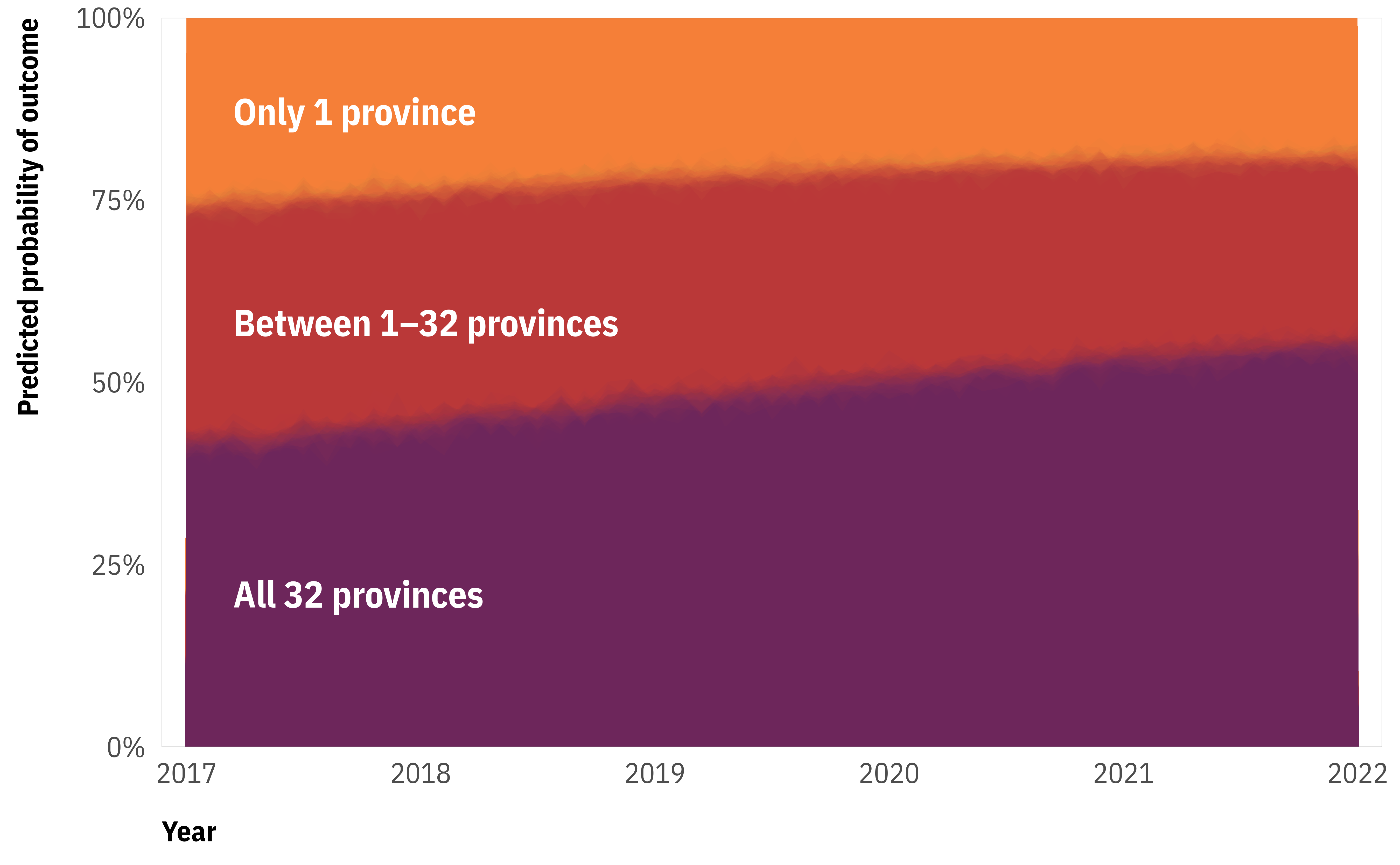
```{r plot-pred-discrete-continuous-timing-area}
preds_timing_plot <- preds_timing |>
  unnest(preds) |>
  mutate(outcome = case_when(
    .prediction == 0 ~ "Only 1 province",
    .prediction > 0 & .prediction < 1 ~ "Between 1–32 provinces",
    .prediction == 1 ~ "All 32 provinces",
    .ptype = factor(
      levels = c("Only 1 province", "Between 1–32 provinces", "All 32 provinces"),
      ordered = TRUE)
  )) |>
  mutate(years_since_law = 2017 + years_since_law) |>
  group_by(outcome, years_since_law, draw) |>
  summarize(count = n()) |>
  group_by(years_since_law) |>
  mutate(prop = count / sum(count) * 100)

layers <- preds_timing_plot |>
  filter(draw <= 50) |>
  split(~ draw) |>
  lapply(\(x) {
    geom_area(
      data = x,
      aes(y = prop, fill = outcome),
      alpha = 0.05
    )
  })

preds_timing_text <- preds_timing_plot |>
  filter(years_since_law == 2017.2) |>
  group_by(outcome) |>
  summarize(median_prop = median_qi(prop)) |>
  unnest(median_prop) |>
  mutate(y_plot = (y / 2) + lag(cumsum(y), default = 0)) |>
  mutate(y_plot = 1 - y_plot) |>
  mutate(years_since_law = 2017.2)

ggplot(preds_timing_plot, aes(x = years_since_law)) +
  layers +
  geom_text(
    data = preds_timing_text,
    aes(y = y_plot, label = outcome),
    color = "white",
    hjust = 0, fontface = "bold", size = 4, show.legend = FALSE
  ) +
  scale_x_continuous(expand = expansion(mult = 0.02)) +
  scale_y_continuous(labels = label_percent(), expand = c(0, 0)) +
  scale_color_manual(values = colorspace::darken(clrs[c(3, 5, 7)], 0.1)) +
  scale_fill_manual(values = colorspace::lighten(clrs[c(3, 5, 7)], 0)) +
  labs(x = "Year", y = "Predicted probability of outcome") +
  guides(fill = "none") +
  theme_ongo() +
  theme(
    panel.grid.major = element_blank()
  )
```