library(tidyverse)library(targets)library(scales)library(glue)library(gt)library(gtExtras)library(modelsummary)library(ggtext)library(brms)library(tidybayes)library(patchwork)# Generated via random.orgset.seed(196491)# Load targetstar_load(ongo)tar_load(c(m_full_ordbeta, m_full_ordbeta_interaction))invisible(list2env(tar_read(graphic_functions), .GlobalEnv))invisible(list2env(tar_read(table_functions), .GlobalEnv))theme_set(theme_ongo())set_annotation_fonts()
Model definition
\[
\begin{aligned}
&\ \textbf{Registered provinces for INGO } i \\
\text{Count of provinces}\ \sim&\ \operatorname{Ordered\,Beta}(\mu_i, \phi_y, k_{1_y}, k_{2_y}) \\[8pt]
&\ \textbf{Model of outcome average} \\
% Put the huge equation in a nested \begin{aligned}[t] environment so that
% \mathrlap{} can go around it so that the annotations in the priors can be
% aligned closer to the math
\mu_i =&\
\mathrlap{\begin{aligned}[t]
& \beta_0 + \beta_1\ \text{Issue[Arts and culture]} + \beta_2\ \text{Issue[Education]}\ +\\
& \beta_3\ \text{Issue[Industry association]} + \beta_4\ \text{Issue[Economy and trade]}\ + \\
& \beta_5\ \text{Issue[Charity and humanitarian]} + \beta_6\ \text{Issue[General]}\ + \\
& \beta_7\ \text{Issue[Health]} + \beta_8\ \text{Issue[Environment]}\ + \\
& \beta_9\ \text{Issue[Science and technology]} + \beta_{10}\ \text{Local connections}\ + \\
& \beta_{11}\ \text{Time since January 2017} + \beta_{12}\ \text{Year registered}
\end{aligned}}\\[8pt]
&\ \textbf{Priors} \\
\beta_0\ \sim&\ \operatorname{Student\,t}(\nu = 3, \mu = 0, \sigma = 2.5) && \text{Intercept} \\
\beta_{1..12}\ \sim&\ \mathcal{N}(0, 5) && \text{Coefficients} \\
\phi_y\ \sim&\ \operatorname{Exponential}(1 / 100) && \text{Variability in province count} \\
k_{1_y}, k_{2_y}\ \sim&\ \operatorname{Induced\,Dirichlet}(1, 1, 1), && \text{0–continuous and continuous–1 cutpoints} \\
&\ \quad \text{or } \bigl[P(\alpha_1), P(\alpha_1 + \alpha_2)\bigr] && \quad\text{(boundaries between 3 Dirichlet columns)}
\end{aligned}
\]
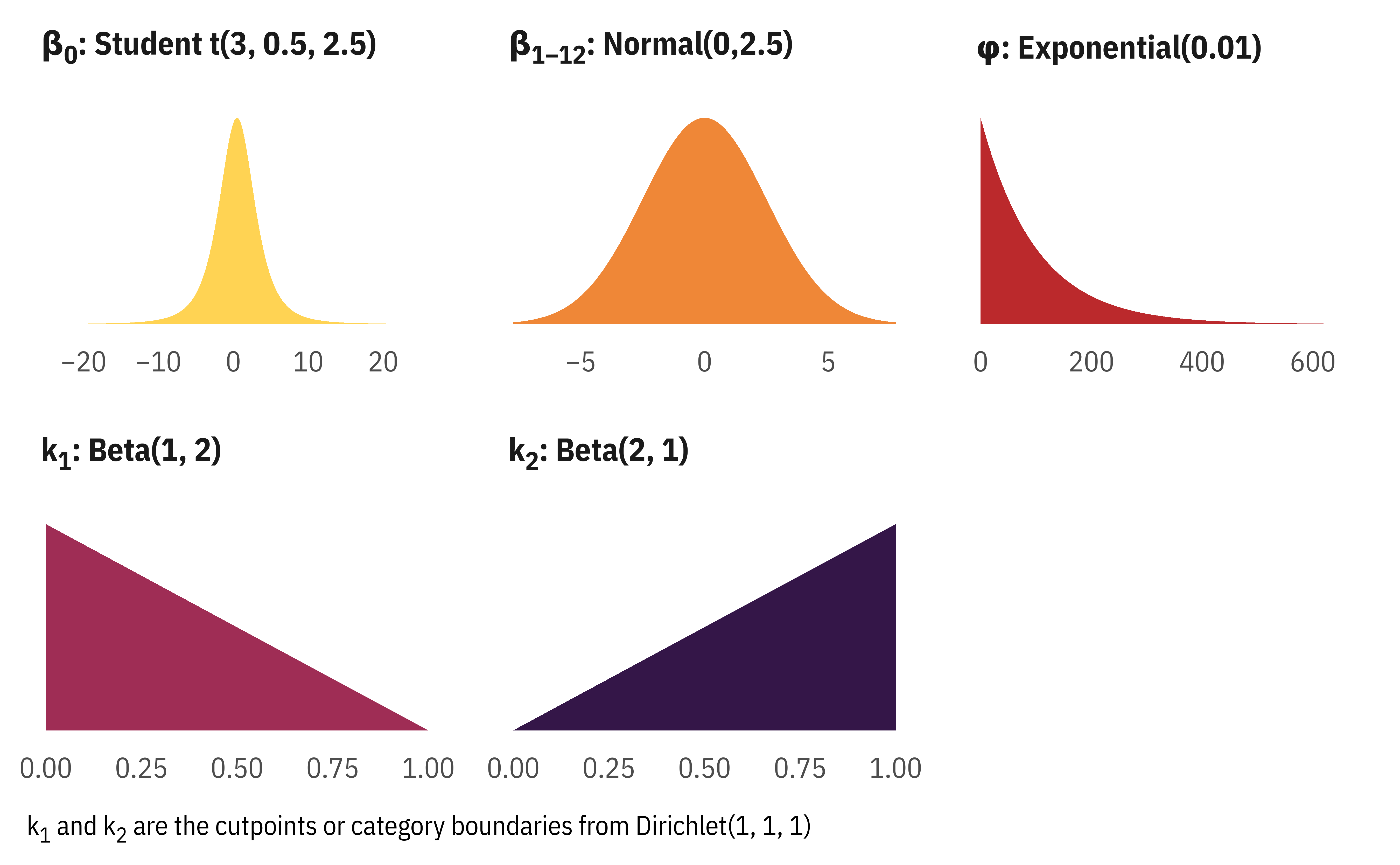
Model priors
These are all pretty standard. I’d like to use a Student t for the coefficients in addition to the intercept, but the prior distributional families are baked into ordbetareg() and the only way to change them is to create a custom {brms} family based on the code in ordbetareg() and that’s a lot of hassle. So we’ll live with a normal distribution for the coefficients.
The only new-to-me distribution here is the Dirichlet prior for the cutpoints, so I wrote a whole blog post about it here. This is a little confusing, though. ordbetareg() requires a three-element Dirichlet distribution that contains three columns of probabilities, one per submodel: the only-zero part, the between-zero-and-one part, and the only-one part. However, it doesn’t use these three probabilities directly. Instead, it uses an induced Dirichlet distribution(Kubinec 2022, 524), meaning that it works with the boundaries between the categories and not the Dirichlet columns themselves (see here for more about that, plus some neat visualizations of the cutpoints).
\(\operatorname{Dirichlet}(1, 1, 1)\) represents a uniform distribution of three related columns in a matrix, each with a probability of 33%, since the sum of the three probabilities must be 100%.
We can find the distributions of the boundaries between these columns too—\(k_1\), or the boundary between the \(\alpha_1\) and \(\alpha_2\) columns, is immediately after \(\alpha_1\), or at 0.33; \(k_2\), or the boundary between \(\alpha_2\) and \(\alpha_3\), is immediately after \(\alpha_2\), which is at (\(\alpha_1 + \alpha_2\)), or 0.66. Because Dirichlet is just a fancy multivariate version of a Beta distribution, each of the \(\alpha\) columns by itself is a Beta distribution, and by extension, the \(k\) boundaries between the \(\alpha\) columns are also Beta distributions:
models <-tribble(~model_name, ~model,"Full model", m_full_ordbeta,"Model with local connections × time interaction", m_full_ordbeta_interaction) |>mutate(duration =map(model, ~{ .$fit |> rstan::get_elapsed_time() |>as_tibble() |>summarize(total =as.duration(max(warmup + sample))) })) |>select(-model) |>unnest(duration)dur <-as.period(as.duration(sum(models$total)))total_run_time <-glue("{hours} hours, {minutes} minutes, and {seconds} seconds",hours =hour(dur), minutes =minute(dur), seconds =round(second(dur), 0))
We ran these models on a 2021 M1 MacBook Pro with 32 GB of RAM, with 4 MCMC chains spread across 8 cores, with two CPU threads per chain, using Stan through brms through cmdstanr.
In total, it took 0 hours, 0 minutes, and 12 seconds to run everything.
Kubinec, Robert. 2022. “Ordered Beta Regression: A Parsimonious, Well-Fitting Model for Continuous Data with Lower and Upper Bounds.”Political Analysis, 1–18. https://doi.org/10.31235/osf.io/2sx6y.
Source Code
---title: Model details and results---```{r setup, include=FALSE}knitr::opts_chunk$set(fig.align = "center", fig.retina = 3, fig.width = 6, fig.height = (6 * 0.618), out.width = "80%", collapse = TRUE, dev = "png", dev.args = list(type = "cairo-png"))options(digits = 3, width = 120, dplyr.summarise.inform = FALSE, knitr.kable.NA = "")``````{r load-libraries, warning=FALSE, message=FALSE}library(tidyverse)library(targets)library(scales)library(glue)library(gt)library(gtExtras)library(modelsummary)library(ggtext)library(brms)library(tidybayes)library(patchwork)# Generated via random.orgset.seed(196491)# Load targetstar_load(ongo)tar_load(c(m_full_ordbeta, m_full_ordbeta_interaction))invisible(list2env(tar_read(graphic_functions), .GlobalEnv))invisible(list2env(tar_read(table_functions), .GlobalEnv))theme_set(theme_ongo())set_annotation_fonts()```# Model definition$$\begin{aligned}&\ \textbf{Registered provinces for INGO } i \\\text{Count of provinces}\ \sim&\ \operatorname{Ordered\,Beta}(\mu_i, \phi_y, k_{1_y}, k_{2_y}) \\[8pt]&\ \textbf{Model of outcome average} \\% Put the huge equation in a nested \begin{aligned}[t] environment so that % \mathrlap{} can go around it so that the annotations in the priors can be % aligned closer to the math\mu_i =&\ \mathrlap{\begin{aligned}[t] & \beta_0 + \beta_1\ \text{Issue[Arts and culture]} + \beta_2\ \text{Issue[Education]}\ +\\ & \beta_3\ \text{Issue[Industry association]} + \beta_4\ \text{Issue[Economy and trade]}\ + \\ & \beta_5\ \text{Issue[Charity and humanitarian]} + \beta_6\ \text{Issue[General]}\ + \\ & \beta_7\ \text{Issue[Health]} + \beta_8\ \text{Issue[Environment]}\ + \\ & \beta_9\ \text{Issue[Science and technology]} + \beta_{10}\ \text{Local connections}\ + \\ & \beta_{11}\ \text{Time since January 2017} + \beta_{12}\ \text{Year registered} \end{aligned}}\\[8pt]&\ \textbf{Priors} \\\beta_0\ \sim&\ \operatorname{Student\,t}(\nu = 3, \mu = 0, \sigma = 2.5) && \text{Intercept} \\\beta_{1..12}\ \sim&\ \mathcal{N}(0, 5) && \text{Coefficients} \\\phi_y\ \sim&\ \operatorname{Exponential}(1 / 100) && \text{Variability in province count} \\k_{1_y}, k_{2_y}\ \sim&\ \operatorname{Induced\,Dirichlet}(1, 1, 1), && \text{0–continuous and continuous–1 cutpoints} \\&\ \quad \text{or } \bigl[P(\alpha_1), P(\alpha_1 + \alpha_2)\bigr] && \quad\text{(boundaries between 3 Dirichlet columns)}\end{aligned}$$# Model priorsThese are all pretty standard. I'd like to use a Student t for the coefficients in addition to the intercept, but the prior distributional families are baked into `ordbetareg()` and the only way to change them is to create a custom {brms} family based on the code in `ordbetareg()` and that's a lot of hassle. So we'll live with a normal distribution for the coefficients.The only new-to-me distribution here is the Dirichlet prior for the cutpoints, so [I wrote a whole blog post about it here](https://www.andrewheiss.com/blog/2023/09/18/understanding-dirichlet-beta-intuition/). This is a little confusing, though. `ordbetareg()` requires a three-element Dirichlet distribution that contains three columns of probabilities, one per submodel: the only-zero part, the between-zero-and-one part, and the only-one part. However, it doesn't use these three probabilities directly. Instead, it uses an [*induced* Dirichlet distribution](https://betanalpha.github.io/assets/case_studies/ordinal_regression.html)[@Kubinec:2022, p. 524], meaning that it works with the *boundaries between the categories* and not the Dirichlet columns themselves ([see here for more about that, plus some neat visualizations of the cutpoints](https://www.andrewheiss.com/blog/2023/09/18/understanding-dirichlet-beta-intuition/#bonus-later-addition-boundaries-between-categories)).$\operatorname{Dirichlet}(1, 1, 1)$ represents a uniform distribution of three related columns in a matrix, each with a probability of 33%, since the sum of the three probabilities must be 100%. $$\begin{align}\textbf{E}(\alpha_1) &= \frac{\alpha_1}{\sum{\alpha}} = \frac{1}{1 + 1 + 1} = \frac{1}{3} = 0.333 \\[8pt]\textbf{E}(\alpha_2) &= \frac{\alpha_2}{\sum{\alpha}} = \frac{1}{1 + 1 + 1} = \frac{1}{3} = 0.333 \\[8pt]\textbf{E}(\alpha_3) &= \frac{\alpha_3}{\sum{\alpha}} = \frac{1}{1 + 1 + 1} = \frac{1}{3} = 0.333\end{align}$$We can find the distributions of the boundaries between these columns too—$k_1$, or the boundary between the $\alpha_1$ and $\alpha_2$ columns, is immediately after $\alpha_1$, or at 0.33; $k_2$, or the boundary between $\alpha_2$ and $\alpha_3$, is immediately after $\alpha_2$, which is at ($\alpha_1 + \alpha_2$), or 0.66. Because Dirichlet is just a fancy multivariate version of a Beta distribution, each of the $\alpha$ columns by itself is a Beta distribution, and by extension, the $k$ boundaries between the $\alpha$ columns are also Beta distributions:$$\begin{align}k_1 &= \textbf{E}(\alpha_1) = \frac{1}{3} & k_2 &= (\textbf{E}(\alpha_2) + \textbf{E}(\alpha_2)) = \frac{2}{3}\\&= \operatorname{Beta}(1, 2) & &= \operatorname{Beta}(2, 1)\end{align}$$So here's what all our priors look like:```{r plot-priors}prior_summary(m_full_ordbeta) |> bind_rows( tibble( prior = c("beta(1, 2)", "beta(2, 1)"), class = c("k1", "k2") ) ) |> parse_dist() |> filter( prior != "", !str_detect(prior, "^induced") ) |> mutate(class_nice = case_match( class, "Intercept" ~ "β<sub>0</sub>", "b" ~ "β<sub>1–12</sub>", "phi" ~ "φ", "k1" ~ "k<sub>1</sub>", "k2" ~ "k<sub>2</sub>" )) |> mutate(prior_nice = str_to_sentence(str_replace(prior, "_", " "))) |> mutate(class = factor(class, levels = c("Intercept", "b", "phi"))) |> arrange(class) |> mutate(nice_title = glue("**{class_nice}**: {prior_nice}")) %>% mutate(nice_title = fct_inorder(nice_title)) %>% ggplot(aes(y = 0, dist = .dist, args = .args, fill = prior)) + stat_slab(normalize = "panels") + scale_x_continuous(labels = label_comma(style_negative = "minus")) + scale_fill_manual(values = clrs[c(6, 8, 5, 3, 1)]) + facet_wrap(vars(nice_title), scales = "free_x", nrow = 2) + guides(fill = "none") + labs( x = NULL, y = NULL, caption = "k<sub>1</sub> and k<sub>2</sub> are the cutpoints or category boundaries from Dirichlet(1, 1, 1)" ) + theme_ongo(prior = TRUE) + theme( strip.text = element_markdown(), plot.caption = element_markdown(hjust = 0) )```# Model run times```{r calculate-model-times}models <- tribble( ~model_name, ~model, "Full model", m_full_ordbeta, "Model with local connections × time interaction", m_full_ordbeta_interaction) |> mutate(duration = map(model, ~{ .$fit |> rstan::get_elapsed_time() |> as_tibble() |> summarize(total = as.duration(max(warmup + sample))) })) |> select(-model) |> unnest(duration)dur <- as.period(as.duration(sum(models$total)))total_run_time <- glue( "{hours} hours, {minutes} minutes, and {seconds} seconds", hours = hour(dur), minutes = minute(dur), seconds = round(second(dur), 0))```We ran these models on a 2021 M1 MacBook Pro with 32 GB of RAM, with 4 MCMC chains spread across 8 cores, with two CPU threads per chain, using Stan through brms through cmdstanr. In total, it took `r total_run_time` to run everything.```{r mcmc-duration-table}#| classes: no-stripemodels |> gt() |> tab_footnote( footnote = "Duration of the longest-running MCMC chain", locations = cells_column_labels(columns = total) ) |> cols_label( model_name = "Model", total = "Total time" ) |> cols_align( align = "left", columns = everything() ) |> fmt_markdown(columns = model_name) |> grand_summary_rows( columns = c(total), fns = list(`Overall total` = ~as.duration(sum(.))) ) |> opt_footnote_marks(marks = "standard") |> opt_horizontal_padding(3) |> opts_theme()```# Model resultsRaw coefficients aren't super useful for interpreting things, but here's a table of them for fun.```{r results-table}#| classes: no-stripemodelsummary( list(m_full_ordbeta, m_full_ordbeta_interaction), statistic = "[{conf.low}, {conf.high}]", ci_method = "hdi", metrics = c("R2"), output = "gt") |> opts_theme()```