To find the causal effects defined in each of our estimands, we calculate estimated marginal means (EMMs) by finding the fitted probability-scale values for each cell in a balanced reference grid of all 576 possible combinations of feature levels (4 organizations × 4 issues × 2 transparency × 2 accountability × 3 funding × 3 government relationship = 576 rows). We then calculate group averages and contrasts in group averages for each of the features of interest, marginalizing over all other features.
This is a little more complicated than just looking at the model coefficients, but it is a valid way of thinking about marginal contrasts and it is a common approach in fields like epidemiology, and the complex multinomial models we’re using require it.
Marginal means, differences in marginal means, marginal effects, and regression coefficients
At its core, a “marginal mean” refers to the literal mean in the margins in a contingency table of model predictions. To illustrate, we’ll make a model that predicts penguin weight based on species and sex and then make predictions for a balanced grid of covariates (i.e. male Adelie, female Adelie, male Chinstrap, female Chinstrap, male Gentoo, female Gentoo):
Code
library(marginaleffects)library(palmerpenguins)penguins <- penguins %>%drop_na(sex)model <-lm(body_mass_g ~ species + sex, data = penguins)preds <- model %>%predictions(datagrid(species = unique, sex = unique))
Code
preds %>%select(estimate, species, sex) %>%pivot_wider(names_from = sex, values_from = estimate) %>%ungroup() %>%gt() %>%cols_label(female ="Female", male ="Male", species ="Species") %>%cols_align(align ="center", columns =c(female, male)) %>%cols_align(align ="left", columns = species) %>%tab_spanner(label ="Sex", columns =c(female, male)) %>%tab_source_note(source_note =md("Predicted penguin weights (g) from model `lm(body_mass_g ~ species + sex)`")) %>%opt_horizontal_padding(3) %>%opts_theme()
Species
Sex
Female
Male
Adelie
3372
4040
Gentoo
4750
5418
Chinstrap
3399
4067
Predicted penguin weights (g) from model lm(body_mass_g ~ species + sex)
We can add a column and row in the margins to show the species-specific and sex-specific average predicted weights. For the sex-specific averages, all the between-species variation is “marginalized out” or accounted for. For the species-specific averages, all the between-sex variation is similarly marginalized out:
Predicted penguin weights (g) from model lm(body_mass_g ~ species + sex)
Because regression is just fancy averages, the differences in marginal means here are actually identical to the coefficients in regression model. For instance, here are the results from the model:
The sexmale coefficient of 667.56 represents the effect of moving from male to female when species is held constant.
The marginal means table shows the same thing. Marginalizing over species (i.e. holding species constant), the average predicted weight for female penguins is 3840.6 and for male penguins is 4508.2. The difference in those marginal means is 667.56—identical to the sexmale coefficient!
Differences in marginal means are equivalent to marginal effects or regression coefficients.
AMCEs from multinomial models
The idea that differences in marginal means can be the same as marginal effects/regression coefficients is crucial for calculating average marginal component effects (AMCEs) with our multinomial conjoint model. With multinomial regression, we actually get three sets of coefficients: one set per conjoint option. Each coefficient shows the shift in probability that someone will choose an organization from column 1, column 2, or column 3, so we get a coefficient for each of those outcomes (or µ1, µ2, and µ3). For instance, here are the posterior median coefficients from our main model for just the funding feature. There are two coefficients (wealthy donors and government grants), but repeated three times (for mu1, mu2, and mu3):
Under experimental conditions where cells in the contingency table are randomly assigned, it’s safe to assume that the cell proportions are equal and then marginalize (i.e. find the average) across the rows or columns. That means we can safely and legally take the average of each set of three coefficients to create a single value per term, like so:
However, these values are on an uninterpretable log odds scale scale and to unlogit them and backtransform them to the probability scale, we need to do all sorts of fancy math involving the intercept terms and omitted levels. That’s tricky and I don’t know how to do it.
So instead, we can take advantage of the fact that regression coefficients are also differences in marginal means. We can create a complete balanced grid of all 576 combinations of feature levels (4 organizations × 4 issues × 2 transparency × 2 accountability × 3 funding × 3 government relationship = 576 rows), calculate predicted probabilities for each row, and then
Here’s what the full grid of 576 options looks like, with posterior median predictions for each combination. Because of the magic of {brms}, these predictions automatically incorporate information from the mu1, mu2, and mu3 versions of the coefficients.
If we want the AMCE of one of the features, like funding, we can calculate the marginal means by grouping by feat_funding and finding the average across each MCMC draw within each type of funding.
Code
mms_funding <- preds_all %>%group_by(feat_funding, .draw) %>%summarize(avg =mean(.epred))mms_funding## # A tibble: 48,000 × 3## # Groups: feat_funding [3]## feat_funding .draw avg## <fct> <int> <dbl>## 1 Funded primarily by many small private donations 1 0.279## 2 Funded primarily by many small private donations 2 0.285## 3 Funded primarily by many small private donations 3 0.283## 4 Funded primarily by many small private donations 4 0.278## 5 Funded primarily by many small private donations 5 0.277## 6 Funded primarily by many small private donations 6 0.285## 7 Funded primarily by many small private donations 7 0.277## 8 Funded primarily by many small private donations 8 0.281## 9 Funded primarily by many small private donations 9 0.281## 10 Funded primarily by many small private donations 10 0.282## # ℹ 47,990 more rows
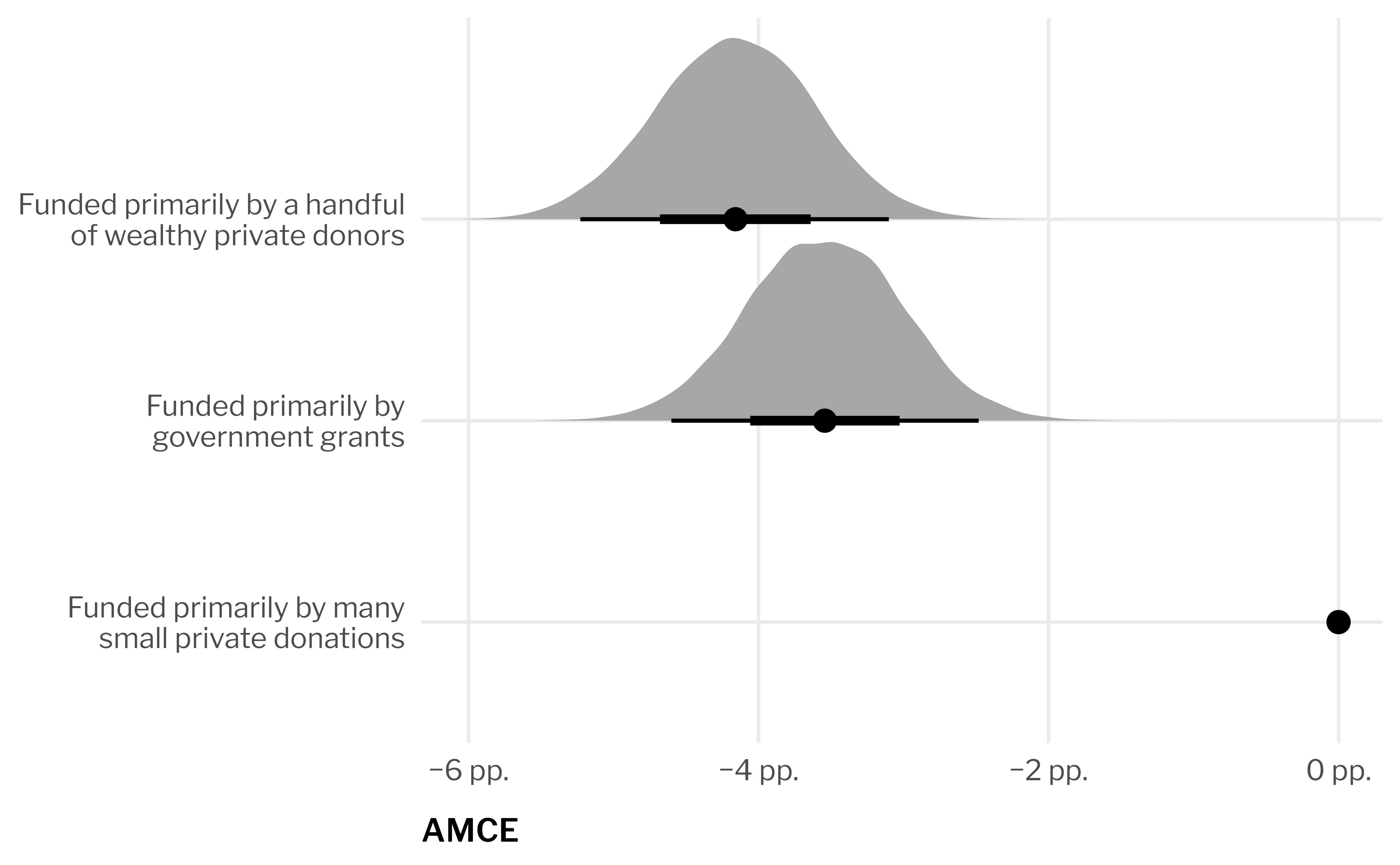
We can then use compare_levels() to find the difference in marginal means, which, as we saw with the penguins example, is the equivalent of looking at a regression coefficient where all other variables in the contingency table (i.e. organization, transparency, accountability, and government relations) are held constant. This gives us the average marginal component effect for funding on the probability scale:
Code
amces_funding <- mms_funding %>%group_by(feat_funding) %>%compare_levels(variable = avg, by = feat_funding, comparison ="control") %>%ungroup() %>%separate_wider_delim( feat_funding,delim =" - ", names =c("feature_level", "reference_level") ) %>%add_row(avg =0, feature_level =unique(.$reference_level))amces_funding %>%group_by(feature_level) %>%median_qi(avg)## # A tibble: 3 × 7## feature_level avg .lower .upper .width .point .interval## <chr> <dbl> <dbl> <dbl> <dbl> <chr> <chr> ## 1 Funded primarily by a handful of wealthy private donors -0.0416 -0.0523 -0.0310 0.95 median qi ## 2 Funded primarily by government grants -0.0354 -0.0460 -0.0248 0.95 median qi ## 3 Funded primarily by many small private donations 0 0 0 0.95 median qiamces_funding %>%mutate(feature_level =fct_rev(fct_inorder(feature_level))) %>%ggplot(aes(x = avg, y = feature_level)) +stat_halfeye() +scale_x_continuous(labels = label_pp) +scale_y_discrete(labels = scales::label_wrap(30)) +labs(x ="AMCE", y =NULL)
AMCEs with covariates
By relying on marginal means, we can also incorporate information about individual-level covariates by creating larger reference grids. For instance, if we want to know how the AMCE for funding varies across different levels of respondent education, we can repeat the 576-row reference grid for each level of education, then group and summarize across funding and education. See the AMCEs section in part 3 of this blog post for more about that.
Source Code
---title: "Why marginal means"format: html: code-fold: true---```{r setup, include=FALSE}knitr::opts_chunk$set(fig.align ="center", fig.retina =3,fig.width =6, fig.height = (6*0.618),out.width ="80%", collapse =TRUE,dev ="ragg_png")options(digits =3, width =120,dplyr.summarise.inform =FALSE,knitr.kable.NA ="")``````{r libraries-data, warning=FALSE, message=FALSE}library(tidyverse)library(targets)library(tidybayes)library(gt)library(gtExtras)tar_config_set(store = here::here("_targets"),script = here::here("_targets.R"))preds_all <-tar_read(preds_conditional_treatment_only)conjoint_model <-tar_read(m_treatment_only)invisible(list2env(tar_read(graphic_functions), .GlobalEnv))invisible(list2env(tar_read(table_functions), .GlobalEnv))theme_set(theme_ngo())```To find the causal effects defined in each of our estimands, we calculate estimated marginal means (EMMs) by finding the fitted probability-scale values for each cell in a balanced reference grid of all 576 possible combinations of feature levels (4 organizations × 4 issues × 2 transparency × 2 accountability × 3 funding × 3 government relationship = 576 rows). We then calculate group averages and contrasts in group averages for each of the features of interest, marginalizing over all other features.This is a little more complicated than just looking at the model coefficients, but it is a valid way of thinking about marginal contrasts and it is a common approach in fields like epidemiology, and the complex multinomial models we're using require it.## Marginal means, differences in marginal means, marginal effects, and regression coefficientsAt its core, a "marginal mean" refers to the literal mean in the margins in a contingency table of model predictions. To illustrate, we'll make a model that predicts penguin weight based on species and sex and then make predictions for a balanced grid of covariates (i.e. male Adelie, female Adelie, male Chinstrap, female Chinstrap, male Gentoo, female Gentoo):```{r make example model}#| code-fold: showlibrary(marginaleffects)library(palmerpenguins)penguins <- penguins %>%drop_na(sex)model <-lm(body_mass_g ~ species + sex, data = penguins)preds <- model %>%predictions(datagrid(species = unique, sex = unique))``````{r basic-contingency-table}preds %>%select(estimate, species, sex) %>%pivot_wider(names_from = sex, values_from = estimate) %>%ungroup() %>%gt() %>%cols_label(female ="Female", male ="Male", species ="Species") %>%cols_align(align ="center", columns =c(female, male)) %>%cols_align(align ="left", columns = species) %>%tab_spanner(label ="Sex", columns =c(female, male)) %>%tab_source_note(source_note =md("Predicted penguin weights (g) from model `lm(body_mass_g ~ species + sex)`")) %>%opt_horizontal_padding(3) %>%opts_theme()```We can add a column and row in the margins to show the species-specific and sex-specific average predicted weights. For the sex-specific averages, all the between-species variation is "marginalized out" or accounted for. For the species-specific averages, all the between-sex variation is similarly marginalized out:```{r fancy-mm-contingency-table}mean_species <- preds %>%group_by(species) %>%summarize(avg_estimate =mean(estimate))mean_sex <- preds %>%group_by(sex) %>%mutate(avg_estimate =mean(estimate)) %>%select(species, sex, estimate, avg_estimate) %>%pivot_wider(names_from = species, values_from = estimate) %>%mutate(avg_explanation = glue::glue("{round(avg_estimate, 0)}<br><span style='font-size:70%'>({round(Adelie, 0)} + {round(Chinstrap, 0)} + {round(Gentoo, 0)}) / 3</span>" )) %>%select(sex, avg_explanation) %>%mutate(species ="**Marginal mean**") %>%pivot_wider(names_from = sex, values_from = avg_explanation)preds %>%ungroup() %>%select(estimate, species, sex) %>%pivot_wider(names_from = sex, values_from = estimate) %>%left_join(mean_species, by =join_by(species)) %>%arrange(species) %>%mutate(avg_explanation = glue::glue("{round(avg_estimate, 0)}<br><span style='font-size:70%'>({round(female, 0)} + {round(male, 0)}) / 2</span>" )) %>%mutate(across(c(female, male), ~as.character(round(., 0)))) %>%select(-avg_estimate) %>%bind_rows(mean_sex) %>%gt() %>%sub_missing(columns =everything(), missing_text ="") %>%fmt_markdown(columns =everything()) %>%cols_label(female ="Female", male ="Male", species ="Species", avg_explanation ="Marginal mean" ) %>%cols_align(align ="center", columns =c(female, male, avg_explanation)) %>%cols_align(align ="left", columns = species) %>%tab_spanner(label ="Sex", columns =c(female, male)) %>%gt_add_divider(columns = avg_explanation, style ="dashed", weight =px(1), sides ="left") %>%tab_style(style =cell_borders(sides ="top", style ="dashed", weight =px(1)),locations =cells_body(rows =4) ) %>%tab_style(style =cell_text(v_align ="top"),locations =cells_body() ) %>%tab_source_note(source_note =md("Predicted penguin weights (g) from model `lm(body_mass_g ~ species + sex)`")) %>%opt_horizontal_padding(3) %>%opts_theme()``````{r extract-sex-means, include=FALSE}mean_sex_small <- preds %>%group_by(sex) %>%summarize(avg_estimate =mean(estimate)) %>%split(~sex)```Because regression is just fancy averages, the differences in marginal means here are actually identical to the coefficients in regression model. For instance, here are the results from the model:```{r show-model-results}#| code-fold: showmodel %>% broom::tidy()```The `sexmale` coefficient of `r round(filter(broom::tidy(model), term == "sexmale")$estimate, 2)` represents the effect of moving from male to female when species is held constant. The marginal means table shows the same thing. Marginalizing over species (i.e. holding species constant), the average predicted weight for female penguins is `r round(mean_sex_small$female$avg_estimate, 1)` and for male penguins is `r round(mean_sex_small$male$avg_estimate, 1)`. The difference in those marginal means is `r round(mean_sex_small$male$avg_estimate - mean_sex_small$female$avg_estimate, 2)`—identical to the `sexmale` coefficient! **Differences in marginal means are equivalent to marginal effects or regression coefficients.** ## AMCEs from multinomial modelsThe idea that differences in marginal means can be the same as marginal effects/regression coefficients is crucial for calculating average marginal component effects (AMCEs) with our multinomial conjoint model. With multinomial regression, we actually get three sets of coefficients: one set per conjoint option. Each coefficient shows the shift in probability that someone will choose an organization from column 1, column 2, or column 3, so we get a coefficient for each of those outcomes (or µ1, µ2, and µ3). For instance, here are the posterior median coefficients from our main model for just the funding feature. There are two coefficients (wealthy donors and government grants), but repeated three times (for `mu1`, `mu2`, and `mu3`):```{r show-funding-mus}#| code-fold: showconjoint_model %>%gather_draws(`^b_mu\\d_feat_funding.*`, regex =TRUE) %>%group_by(.variable) %>%median_qi(.value)```Under experimental conditions where cells in the contingency table are randomly assigned, it's safe to assume that the cell proportions are equal and then marginalize (i.e. find the average) across the rows or columns. That means we can safely and legally take the average of each set of three coefficients to create a single value per term, like so:```{r show-funding-mus-collapsed}#| code-fold: showconjoint_model %>%gather_draws(`^b_mu\\d_feat_funding.*`, regex =TRUE) %>%mutate(.variable =str_remove(.variable, "_mu\\d")) %>%group_by(.variable) %>%median_qi(.value)```However, these values are on an uninterpretable log odds scale scale and to unlogit them and backtransform them to the probability scale, we need to do all sorts of fancy math involving the intercept terms and omitted levels. That's tricky and I don't know how to do it.So instead, we can take advantage of the fact that regression coefficients are also differences in marginal means. We can create a complete balanced grid of all 576 combinations of feature levels (4 organizations × 4 issues × 2 transparency × 2 accountability × 3 funding × 3 government relationship = 576 rows), calculate predicted probabilities for each row, and then Here's what the full grid of 576 options looks like, with posterior median predictions for each combination. Because of the magic of {brms}, these predictions automatically incorporate information from the `mu1`, `mu2`, and `mu3` versions of the coefficients.```{r show-full-grid-preds}#| column: screenpreds_all %>%group_by(feat_org, feat_issue, feat_transp, feat_acc, feat_funding, feat_govt) %>%summarize(avg =mean(.epred)) %>%ungroup() %>%gt() %>%cols_align(align ="left") %>%cols_label(feat_org ="Organization",feat_issue ="Issue",feat_transp ="Transparency",feat_acc ="Accountability",feat_funding ="Funding",feat_govt ="Relationship",avg ="Median probability" ) %>%opts_theme() %>%opt_interactive(use_compact_mode =TRUE, use_highlight =TRUE, use_filters =TRUE)```\ If we want the AMCE of one of the features, like funding, we can calculate the marginal means by grouping by `feat_funding` and finding the average across each MCMC draw within each type of funding. ```{r calc-mms-funding}#| code-fold: showmms_funding <- preds_all %>%group_by(feat_funding, .draw) %>%summarize(avg =mean(.epred))mms_funding```We can then use `compare_levels()` to find the difference in marginal means, which, as we saw with the penguins example, is the equivalent of looking at a regression coefficient where all other variables in the contingency table (i.e. organization, transparency, accountability, and government relations) are held constant. This gives us the average marginal component effect for funding *on the probability scale*:```{r show-amces-funding}#| code-fold: showamces_funding <- mms_funding %>%group_by(feat_funding) %>%compare_levels(variable = avg, by = feat_funding, comparison ="control") %>%ungroup() %>%separate_wider_delim( feat_funding,delim =" - ", names =c("feature_level", "reference_level") ) %>%add_row(avg =0, feature_level =unique(.$reference_level))amces_funding %>%group_by(feature_level) %>%median_qi(avg)amces_funding %>%mutate(feature_level =fct_rev(fct_inorder(feature_level))) %>%ggplot(aes(x = avg, y = feature_level)) +stat_halfeye() +scale_x_continuous(labels = label_pp) +scale_y_discrete(labels = scales::label_wrap(30)) +labs(x ="AMCE", y =NULL)```## AMCEs with covariatesBy relying on marginal means, we can also incorporate information about individual-level covariates by creating larger reference grids. For instance, if we want to know how the AMCE for funding varies across different levels of respondent education, we can repeat the 576-row reference grid for each level of education, then group and summarize across funding and education. See [the AMCEs section in part 3 of this blog post](https://www.andrewheiss.com/blog/2023/08/12/conjoint-multilevel-multinomial-guide/#amces-2) for more about that.