Bayesian models
Suparna Chaudhry and Andrew Heiss
2018-10-29
knitr::opts_chunk$set(cache = FALSE, fig.retina = 2,
                      tidy.opts = list(width.cutoff = 120),  # For code
                      options(width = 120))  # For output

library(tidyverse)
library(stringr)
library(forcats)
library(stargazer)
library(huxtable)
library(lme4)
library(modelr)
library(broom)
library(broom.mixed)
library(scales)
library(formula.tools)
library(here)

source(here("lib", "graphics.R"))
source(here("lib", "pandoc.R"))
source(here("lib", "bayes.R"))

source(here("lib", "robustness_models_definitions.R"))
source(here("lib", "h1_model_definitions.R"))
source(here("lib", "h2_model_definitions.R"))
source(here("lib", "h3_model_definitions.R"))

my.seed <- 1234
set.seed(my.seed)
df.country.aid <- readRDS(here("Data", "data_clean",
"df_country_aid_no_imputation.rds"))
df.country.aid.impute <- readRDS(here("Data", "data_clean",
"df_country_aid_imputation.rds"))
df.country.aid.impute.m10 <- readRDS(here("Data", "data_clean",
"df_country_aid_imputation_m10.rds"))
dcjw.questions.clean <- read_csv(here("Data", "data_manual", "dcjw_questions.csv"))
dcjw.responses.clean <- read_csv(here("Data", "data_manual", "dcjw_responses.csv"))
# Load clean coefficient names and append "within" and "between" to them,
# resulting in a giant table of possible coefficient names
coef.names <- read_csv(here("Data", "data_manual", "coef_names.csv"))
coef.names.within <- coef.names %>%
mutate(term = paste0(term, "_within"),
term_plot = paste0(term_clean, "\n(within)"),
term_plot_short = term_clean,
term_clean = paste0(term_clean, "~within~"))
coef.names.between <- coef.names %>%
mutate(term = paste0(term, "_between"),
term_plot = paste0(term_clean, "\n(between)"),
term_plot_short = paste0(term_clean, ""),
term_clean = paste0(term_clean, "~between~"))
coef.names.all <- bind_rows(coef.names, coef.names.within, coef.names.between) %>%
mutate_at(vars(term_plot, term_plot_short),
funs(ifelse(is.na(.), term_clean, .))) %>%
mutate(term_plot_short = recode(term_plot_short,
`Civil society reg. env. (CSRE)` = "CSRE"))
# Load clean model names
model.names <- read_csv(here("Data", "data_manual", "model_names.csv"))
# Combine original data and imputed data so calculations can happen at the same time
df.country.aid.both <- bind_rows(df.country.aid, df.country.aid.impute)
# Combine m=10 imputed data too since we use it in some robustness checks.
# Imputations 6-10 are later removed
df.country.aid.all <- bind_rows(df.country.aid, df.country.aid.impute.m10)
# All the missing values have been taken care of, but final years for leaded
# variables *are* still missing (i.e. there's no aid data for 2014, so
# total.oda_log_next_year will be NA in 2013). For this fancy random effects
# regression to work, the demeaned variables have to be based on the means of
# all rows included in the regression, so they can't include rows that are
# dropped because of missingness. This means we have to make separate demeaned
# datasets for *_after_2 and *_after_5, but ¯\_(ツ)_/¯
df.country.aid.demean.next_year.all <- df.country.aid.all %>%
filter(!is.na(total.oda_log_next_year)) %>%
group_by(m, cowcode) %>%
mutate_at(vars(barriers.total, advocacy, entry, funding,
polity, gdp.capita_log, gdp.capita, trade.pct.gdp, corruption, csre,
total.oda_log),
funs(between = mean(., na.rm = TRUE), # meaned
within = . - mean(., na.rm = TRUE))) %>% # demeaned
ungroup()
df.country.aid.us.demean.next_year.all <- df.country.aid.all %>%
filter(!is.na(prop.ngo.dom_logit_next_year)) %>%
filter(year > 1999) %>%
group_by(m, cowcode) %>%
mutate_at(vars(barriers.total, advocacy, entry, funding,
polity, gdp.capita_log, gdp.capita, trade.pct.gdp, corruption, csre,
total.oda_log),
funs(between = mean(., na.rm = TRUE), # meaned
within = . - mean(., na.rm = TRUE))) %>% # demeaned
ungroup()
# Divide demeaned data into separate data frames: original, imputed (m=5), and imputed (m=10)
df.country.aid.demean.next_year.both <-
filter(df.country.aid.demean.next_year.all, !(m %in% paste0("imp", 6:10)))
df.country.aid.demean.next_year <-
filter(df.country.aid.demean.next_year.all, m == "original")
df.country.aid.us.demean.next_year.both <-
filter(df.country.aid.us.demean.next_year.all, !(m %in% paste0("imp", 6:10)))
df.country.aid.us.demean.next_year <-
filter(df.country.aid.us.demean.next_year.all, m == "original")
df.country.aid.demean.next_year.impute <-
filter(df.country.aid.demean.next_year.all,
m != "original", !(m %in% paste0("imp", 6:10)))
df.country.aid.demean.next_year.impute.m10 <-
filter(df.country.aid.demean.next_year.all, m != "original")
# Demean data with total.oda_log leaded by 2 years and 5 years
# After 2 years
df.country.aid.demean.after_2.both <- df.country.aid.both %>%
filter(!is.na(total.oda_log_after_2)) %>%
group_by(m, cowcode) %>%
mutate_at(vars(barriers.total, advocacy, entry, funding,
polity, gdp.capita_log, gdp.capita, trade.pct.gdp, corruption, csre,
total.oda_log),
funs(between = mean(., na.rm = TRUE), # meaned
within = . - mean(., na.rm = TRUE))) %>% # demeaned
ungroup()
df.country.aid.demean.after_2 <-
filter(df.country.aid.demean.after_2.both, m == "original")
df.country.aid.demean.after_2.impute <-
filter(df.country.aid.demean.after_2.both, m != "original")
# After 5 years
df.country.aid.demean.after_5.both <- df.country.aid.both %>%
filter(!is.na(total.oda_log_after_5)) %>%
group_by(m, cowcode) %>%
mutate_at(vars(barriers.total, advocacy, entry, funding,
polity, gdp.capita_log, gdp.capita, trade.pct.gdp, corruption, csre,
total.oda_log),
funs(between = mean(., na.rm = TRUE), # meaned
within = . - mean(., na.rm = TRUE))) %>% # demeaned
ungroup()
df.country.aid.demean.after_5 <-
filter(df.country.aid.demean.after_5.both, m == "original")
df.country.aid.demean.after_5.impute <-
filter(df.country.aid.demean.after_5.both, m != "original")h1.raw <- here("Data", "data_cache", "models_bayes_h1.rds")
h2.raw <- here("Data", "data_cache", "models_bayes_h2.rds")
h2.raw.zoib <- here("Data", "data_cache", "models_bayes_h2_zoib.rds")
h3.domestic.raw <- here("Data", "data_cache", "models_bayes_h3_domestic.rds")
h3.domestic.raw.zoib <- here("Data", "data_cache", "models_bayes_h3_domestic_zoib.rds")
h3.foreign.raw <- here("Data", "data_cache", "models_bayes_h3_foreign.rds")
h3.foreign.raw.zoib <- here("Data", "data_cache", "models_bayes_h3_foreign_zoib.rds")
if (file.exists(h1.raw) & file.exists(h2.raw) &
file.exists(h3.domestic.raw) & file.exists(h3.foreign.raw)) {
mods.h1.next_year.raw.bayes <- read_rds(h1.raw)
mods.h2.next_year.raw.bayes <- read_rds(h2.raw)
mods.h2.next_year.raw.bayes.zoib <- read_rds(h2.raw.zoib)
mods.h3.dom.next_year.raw <- read_rds(h3.domestic.raw)
mods.h3.dom.next_year.raw.zoib <- read_rds(h3.domestic.raw.zoib)
mods.h3.foreign.next_year.raw <- read_rds(h3.foreign.raw)
mods.h3.foreign.next_year.raw.zoib <- read_rds(h3.foreign.raw.zoib)
} else {
stop("Run Data/run_bayes_remote.R to generate the model data")
}stars <- function(p) {
out <- symnum(p, cutpoints = c(0, 0.01, 0.05, 0.1, 1),
symbols = c("***", "**", "*", ""))
as.character(out)
}
fixed.digits <- function(x, digits = 2) {
formatC(x, digits = digits, format = "f")
}
# Use 2 significant digits only on the decimal part of the number, ignoring the
# integer part. See my question here: http://stackoverflow.com/q/43050903/120898
# fixed.digits <- function(x, digits = 2) {
# as.character(floor(x) + signif(x %% 1, digits))
# }
# Inverse logit, with the ability to account for adjustments
# via http://stackoverflow.com/a/23845527/120898
inv.logit <- function(f, a) {
a <- (1 - 2 * a)
(a * (1 + exp(f)) + (exp(f) - 1)) / (2 * a * (1 + exp(f)))
}
# Take apart the pieces of a random effects formula and rebuild it
build.formula <- function(DV, IVs) {
terms.all <- attr(terms(IVs), "term.labels")
terms.fixed <- terms.all[!stringr::str_detect(terms.all, "\\|")]
terms.rand <- sapply(findbars(formula(IVs)),function(x) paste0("(", deparse(x), ")"))
reformulate(c(terms.fixed, terms.rand), response = DV)
}
get.rhs <- function(x) rhs.vars(x) %>% str_replace_all("1 \\| ", "")
get.lhs <- function(x) lhs.vars(x)
is_scaled <- function(x) "scaled:scale" %in% names(attributes(x))
get_scale <- function(x) attr(x, "scaled:scale")
# Meld a bunch of imputed models
meld.imputed.models <- function(model.data, exponentiate = FALSE) {
models.df <- model.data$glance[[1]]$df.residual
models.tidy <- model.data %>%
select(tidy) %>%
unnest(.id = "imputation")
just.estimates <- models.tidy %>%
filter(group == "fixed") %>%
select(imputation, term, estimate) %>%
spread(term, estimate) %>%
select(-imputation)
just.ses <- models.tidy %>%
filter(group == "fixed") %>%
select(imputation, term, std.error) %>%
spread(term, std.error) %>%
select(-imputation)
# If no imputed data was passed in, use the actual estimates and SEs
if (nrow(just.estimates) > 1) {
melded <- Amelia::mi.meld(just.estimates, just.ses)
} else {
melded <- list(q.mi = just.estimates, se.mi = just.ses)
}
melded.tidy <- as.data.frame(cbind(t(melded$q.mi),
t(melded$se.mi))) %>%
magrittr::set_colnames(c("estimate", "std.error")) %>%
mutate(term = rownames(.)) %>%
select(term, everything()) %>%
mutate(statistic = estimate / std.error,
conf.low = estimate + std.error * qt(0.025, models.df),
conf.high = estimate + std.error * qt(0.975, models.df),
p.value = 2 * pt(abs(statistic), models.df, lower.tail = FALSE),
stars = stars(p.value))
if (exponentiate) {
# Convert SEs to odds ratios. This isn't entirely 100% accurate, since the
# melded coefficient variances (i.e. diag(vcov(.))) are just averaged, not
# melded with Amelia's fancy mi.meld(), but ¯\_(ツ)_/¯
#
# https://www.andrewheiss.com/blog/2016/04/25/convert-logistic-regression-standard-errors-to-odds-ratios-with-r/
fixed.coefs.var <- model.data %>%
mutate(var.diag = model %>% map(~ diag(vcov(.)))) %>%
select(var.diag, model) %>% unnest(var.diag)
just.var <- models.tidy %>%
filter(group == "fixed") %>%
select(imputation, term) %>%
bind_cols(fixed.coefs.var) %>%
group_by(term) %>%
summarise(var.diag = mean(var.diag))
melded.tidy <- melded.tidy %>%
left_join(just.var, by = "term") %>%
mutate(or = exp(estimate),
or.se = sqrt(or^2 * var.diag),
or.upper = or + (qnorm(0.975) * or.se),
or.lower = or + (qnorm(0.025) * or.se))
}
melded.tidy
}
# Expects a data frame with a column named tidy.melded and a row for model
# names. Term names are based on the first model in the data column for each
# row, and are filtered through stargazer to get the correct row order.
stargazer.fake <- function(df, caption = NULL, note = NULL, exponentiate = FALSE) {
# Create a blank row with a bolded row name
header.row <- function(header) {
data_frame(term = paste0("**", header, "**"),
models = df$model.name, value = "") %>%
spread(models, value)
}
note.row <- function(note) {
crossing(term = note,
models = df$model.name, value = "") %>%
spread(models, value) %>%
# Sort based on original note order
slice(match(note, term))
}
coef.order.models <- df %>%
# Select just the first row of each model
unnest(data) %>%
# Sometimes there are duplicate column names
# magrittr::set_colnames(make.unique(colnames(.))) %>%
# Keep order of model.name
mutate(model.name = ordered(fct_inorder(model.name))) %>%
group_by(model.name) %>%
slice(1) %>% ungroup() %>%
select(model) %>% as.list()
# Use stargazer to get the coefficient order. I tried recreating stargazer's
# coefficient ordering algorithm but it's way too complicated. So instead, we
# cheat and let stargazer do the heavy lifting, save the output to a string,
# and then extract the coefficient names with str_extract. Super super hacky,
# but it works.
#
# See http://stackoverflow.com/a/41801861/120898
capture.output({
stargazer.coefs <- stargazer::stargazer(coef.order.models,
type = "text", table.layout = "t")
}, file = "/dev/null")
coef.order <- setdiff(stringr::str_extract(stargazer.coefs, "^[\\w\\.]*"), c(""))
# Fixed parts
fixed.tidy <- df %>%
unnest(tidy.melded)
if (exponentiate) {
fixed.coefs <- fixed.tidy %>%
mutate(fancy = paste0(fixed.digits(or, 3),
stars, "\\ \n(",
fixed.digits(or.se, 3),
")"))
} else {
fixed.coefs <- fixed.tidy %>%
mutate(fancy = paste0(fixed.digits(estimate, 3),
stars, "\\ \n(",
fixed.digits(std.error, 3),
")"))
}
fixed.coefs <- fixed.coefs %>%
select(model.name, term, fancy) %>%
spread(model.name, fancy, fill = "") %>%
# Clean up term names
mutate(term = stringr::str_replace(term, "TRUE$|FALSE$", ""),
term = recode(term, `(Intercept)` = "Constant")) %>%
# Use stargazer's coefficient order
mutate(term = factor(term, levels = coef.order, ordered = TRUE)) %>%
arrange(term) %>%
mutate(term = as.character(term)) %>%
left_join(coef.names.all, by = "term") %>%
mutate(term_clean = ifelse(term == "Constant", "Constant", term_clean)) %>%
select(-term) %>% rename(term = term_clean) %>%
select_(.dots = c("term", df$model.name))
# Random parts
random.coef.order.raw <- df %>%
unnest(data) %>%
# unnest(data) %>% magrittr::set_colnames(make.unique(colnames(.))) %>%
select(model.name, model) %>%
mutate(ranef = model %>% map(~ as.data.frame(VarCorr(.)))) %>%
unnest(ranef)
random.coef.order <- c(setdiff(unique(random.coef.order.raw$grp), "Residual"), "Residual")
random.coefs <- df %>%
unnest(data) %>%
unnest(tidy) %>%
filter(group != "fixed") %>%
rename(term.raw = term, term = group) %>%
group_by(model.name, term) %>%
summarise(avg.random.sd = mean(estimate),
sd.random.sd = sd(estimate)) %>%
mutate(fancy = paste0(fixed.digits(avg.random.sd, 3),
"\\ \n(",
ifelse(is.na(sd.random.sd), "NA", fixed.digits(sd.random.sd, 3)),
")")) %>%
select(model.name, term, fancy) %>%
spread(model.name, fancy, fill = "") %>%
mutate(term = factor(term, levels = random.coef.order, ordered = TRUE)) %>%
arrange(term) %>% mutate(term = as.character(term)) %>%
left_join(coef.names.all, by = "term") %>%
mutate(term_clean = ifelse(term == "Residual",
"Residual random error ($\\sigma$)", term_clean)) %>%
select(-term) %>% select(term = term_clean, everything())
# Create the bottom half of the table
# Calculate the average log likelihood for all imputed models
avg.loglik <- df %>%
unnest(data) %>% unnest(glance) %>%
group_by(model.name) %>%
summarise(avg.loglik = as.character(round(mean(logLik), 2))) %>%
mutate(term = "Log likelihood (mean)") %>%
spread(model.name, avg.loglik)
# Imputation frames
n.obs <- df %>%
unnest(data) %>%
mutate(n = model %>% map_int(~ nrow(.@frame))) %>%
select(model.name, n) %>%
group_by(model.name) %>% slice(1) %>% ungroup() %>%
mutate(term = "Observations",
n = scales::comma(n)) %>%
spread(model.name, n)
n.m <- df %>%
mutate(m.new = data %>% map_int(~ nrow(.))) %>%
select(model.name, m.new) %>%
mutate(m.new = ifelse(m.new == 1, 0, m.new),
m.new = as.character(m.new)) %>%
mutate(term = "Imputed datasets (*m*)") %>%
spread(model.name, m.new)
bottom.details <- bind_rows(n.obs, avg.loglik, n.m)
if (exponentiate) {
fixed.title <- "Fixed part (odds ratios)"
random.title <- "Random part (original coefficients)"
} else {
fixed.title <- "Fixed part"
random.title <- "Random part"
}
if (!is.null(note)) {
notes <- bind_rows(header.row("Notes"), note.row(note))
} else {
notes <- NULL
}
nice.top.bottom <- bind_rows(header.row(fixed.title), fixed.coefs,
header.row(random.title), random.coefs,
header.row("Model details"), bottom.details,
notes) %>%
select_(.dots = c("term", df$model.name))
# Make column names (1), (2), etc.
# TODO: Allow for custom column names
colnames(nice.top.bottom) <- c(" ", paste0("(", 1:length(df$model.name), ")"))
# All columns are centered except the first
# TODO: MAYBE: Let this be user configurable
table.align <- paste0(c("l", rep("c", length(df$model.name))), collapse = "")
pandoc.table.return(nice.top.bottom, keep.line.breaks = TRUE,
justify = table.align, caption = caption)
}# Wrappers around tidy.stanreg and glance.stanreg so that we can rescale and
# exponentiate coefficients in huxreg
tidy.scalemcmc <- function(x, scalings = NULL, exponentiate = FALSE, ...) {
# This is hacky, but it works. Remove the custom "scalemcmc" class so that
# regular broom functions work on x
class(x) <- class(x)[class(x) != "scalemcmc"]
non_scaled <- tidy(x, ...)
adjusted <- non_scaled %>%
left_join(scalings, by = "term") %>%
gather(column, value, -term, -scaled) %>%
mutate(value_rescaled = ifelse(!is.na(scaled), value / scaled, value)) %>%
select(term, column, value_rescaled) %>%
spread(column, value_rescaled)
if (exponentiate) {
adjusted <- adjusted %>%
mutate_at(vars(-term, -std.error), exp)
}
return(adjusted)
}
glance.scalemcmc <- function(x, ...) {
class(x) <- class(x)[class(x) != "scalemcmc"]
return(glance(x, ...))
}
add_scalemcmc <- function(x) {
class(x) <- c("scalemcmc", class(x))
return(x)
}H1: Donors reduce aid in response to legislation
H1: In response to restrictive NGO legislation, bilateral, multilateral, and private donors may reduce their aid to repressive countries.
\[ln( \text{ODA}_{\text{OECD}} )_{i, t+1} = \text{NGO legislation}_{it} + \text{controls}_{it}\]
Our dependent variable for this hypothesis is the log of ODA (constant 2011 dollars), leaded by one year so we don’t have to lag every other independent variable. As a robustness check, we also include models with log ODA leaded by 2 years and 5 years to account the implementation period following the passage of a law.
We look at NGO legislation in a few different ways:
barriers.total: Number of anti-NGO legal barriers in a country-yearadvocacy + entry + funding: Number of anti-NGO legal barriers by type of barriercsre: Civil society regulatory environment index (CSRE), ranging from roughly -4 to 4 (higher values = better civil society regulations)
# Get scaling factors
scales.h1.next_year <- mods.h1.next_year.raw.bayes %>%
  filter(m != "original") %>%
  select(m, starts_with("scales")) %>%
  gather(scales.name, scales, -m)

# Get model details and parameters
mods.h1.next_year.bayes <- mods.h1.next_year.raw.bayes %>%
  filter(m != "original") %>%
  select(m, starts_with("mod")) %>%
  gather(model.name, model, -m) %>%
  # FOR SOME REASON glance takes forever to calculate three numbers
  mutate(glance = model %>% map(glance),
         tidy = model %>% map(tidy)) %>%
  bind_cols(select(scales.h1.next_year, -m))
MCMC diagnostics
Check fit
We use one of the imputed models (mod.h1.barriers.total) to check for fit and convergence.
model.to.check <- mods.h1.next_year.bayes %>%
  filter(m == "imp1", model.name == "mod.h1.barriers.total") %>%
  select(model) %>% .[[1]] %>% .[[1]]
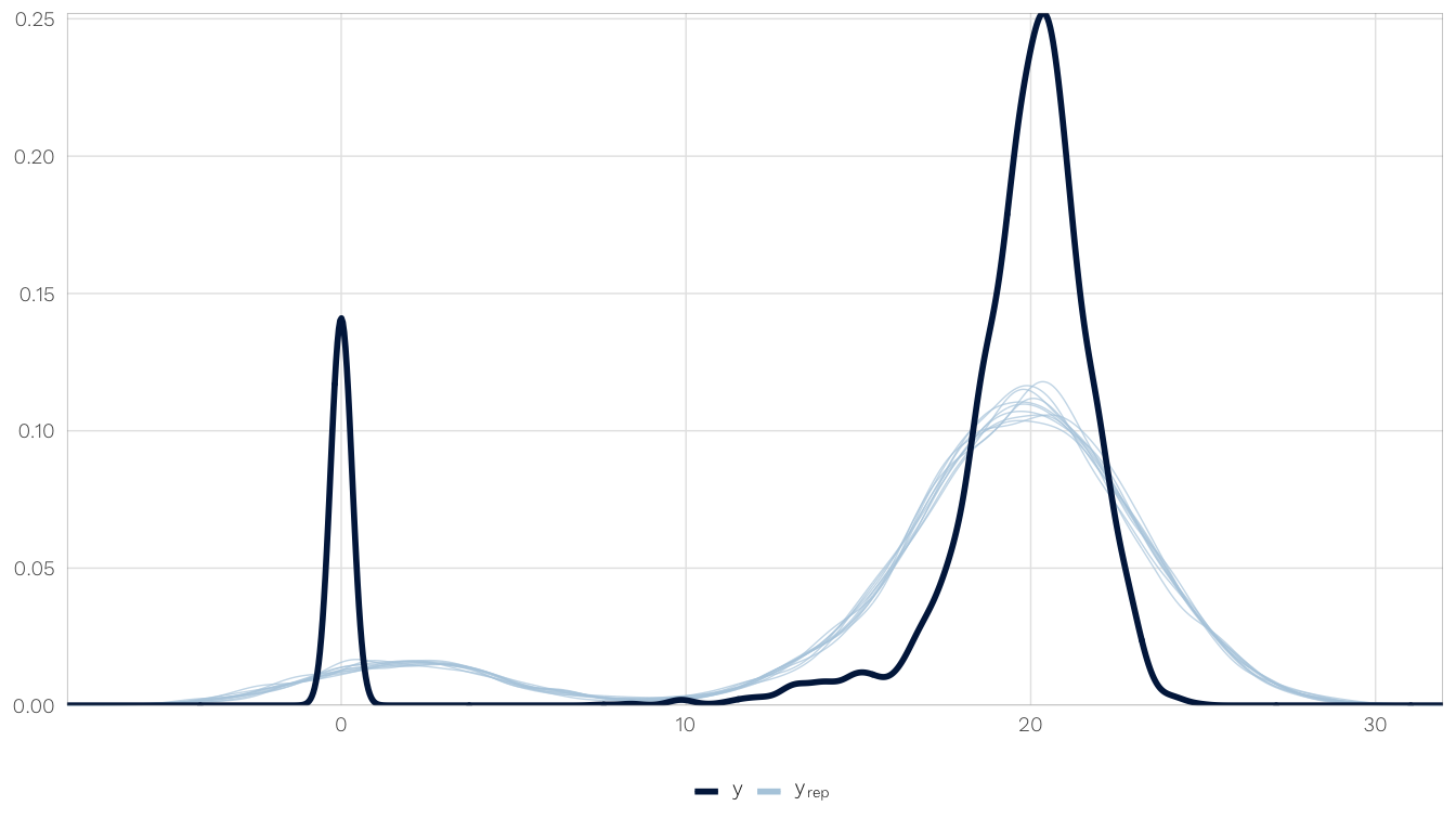
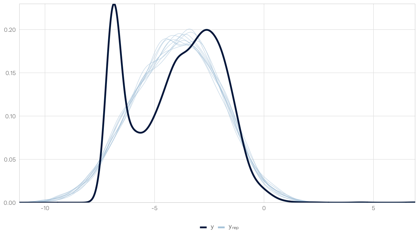
How well does the posterior predictive distribution fit the observed outcome? Not great, but not perfectly. The actual distribution is bimodal, with a bunch of zeros, and the model gets the two peaks, but they’re shallow. We can live with it, though.
Check convergence
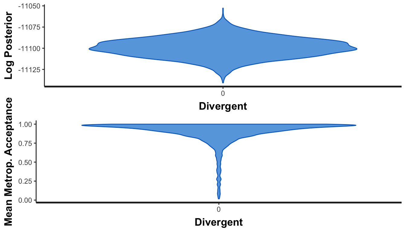
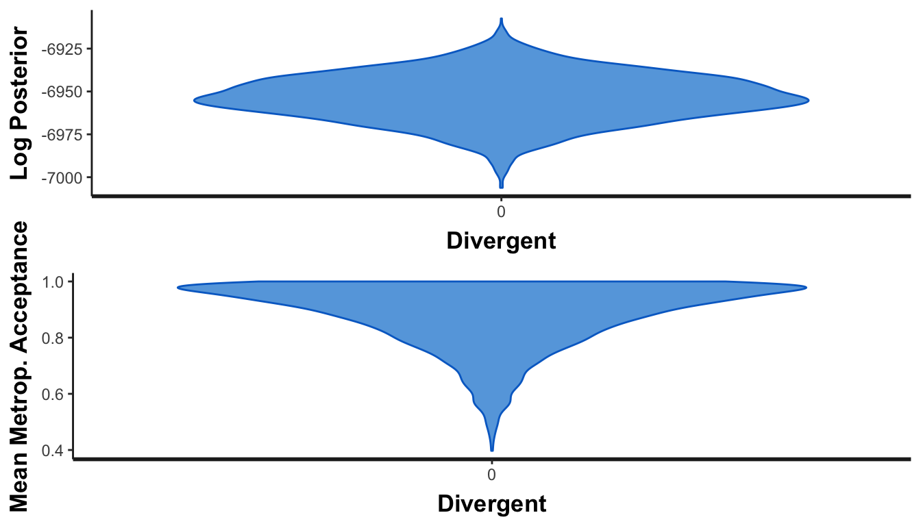
What about chain convergence? These should look like tops if everything converges, with no observations at 0 in the mean Metropolis-Hastings aceptance panel.
Merging MCMC chains
Merging the MCMC chains is relatively easy, but then working with the 20,000 rows of simulations is trickier, since merging makes the model a data_frame intead of a stanreg object, meaning all the convenience funcions like posterior_predict() don’t work anymore. That means lots of math. Ugh.
So instead, we do two things. We calculate the posterior median and MD by just merging all the MCMC chains from all imputations. Becuase posterior_predict() doesn’t work on merged chains like this, we run posterior_predict() on each imputation and then take the mean of each imputation’s credible intervals. This should be okay—taking the median of medians (or mean of means) will yield the same value if the group sizes are the same (thus avoiding Simpson’s Paradox). Like this:
## [1] 4.5## [1] 4.5If it’s a little off, it should be okay—it’ll be off by an order of 0.001ish.
Results
Coefficients
vars.to.plot <- c("barriers.total_within", "barriers.total_between",
                  "advocacy_within", "advocacy_between",
                  "entry_within", "entry_between",
                  "funding_within", "funding_between",
                  "csre_within", "csre_between")

mods.h1.melded <- bayes.meld(mods.h1.next_year.bayes,
                             vars.to.plot)$melded.summary

plot.data <- mods.h1.melded %>%
  left_join(coef.names.all, by = "term") %>%
  left_join(model.names, by = c("model.name" = "model")) %>%
  mutate(coef.type = case_when(
    str_detect(term, "_within") ~ "Within",
    str_detect(term, "_between") ~ "Between",
  )) %>%
  mutate(term = factor(term, levels = vars.to.plot, ordered = TRUE)) %>%
  arrange(desc(term)) %>%
  mutate(term_plot_short = fct_inorder(term_plot_short, ordered = TRUE)) %>%
  mutate(coef.type = factor(coef.type, levels = c("Within", "Between"),
                            ordered = TRUE)) %>%
  mutate(model_clean = factor(model_clean, levels = rev(unique(model_clean)), ordered = TRUE))

fig.coefs.h1 <- ggplot(plot.data, aes(x = med, y = term_plot_short,
                                      xmin = `2.5%`, xmax = `97.5%`, colour = model_clean)) +
  geom_vline(xintercept = 0, colour = "black", size = 0.5) +
  geom_pointrangeh(size = 0.5, fatten = 3) +
  labs(x = "Posterior median change in log ODA in following year", y = NULL) +
  scale_colour_manual(values = model.colors, name = NULL) +
  expand_limits(x = c(-2, 1)) +
  guides(color = guide_legend(override.aes = list(size = 0.25))) +
  theme_donors() +
  theme(legend.justification = "left",
        legend.box.margin = margin(l = -0.75, t = -0.5, unit = "lines"),
        axis.title.x = element_text(hjust = 0)) +
  facet_wrap(~ coef.type, scales = "free", ncol = 2)
fig.coefs.h1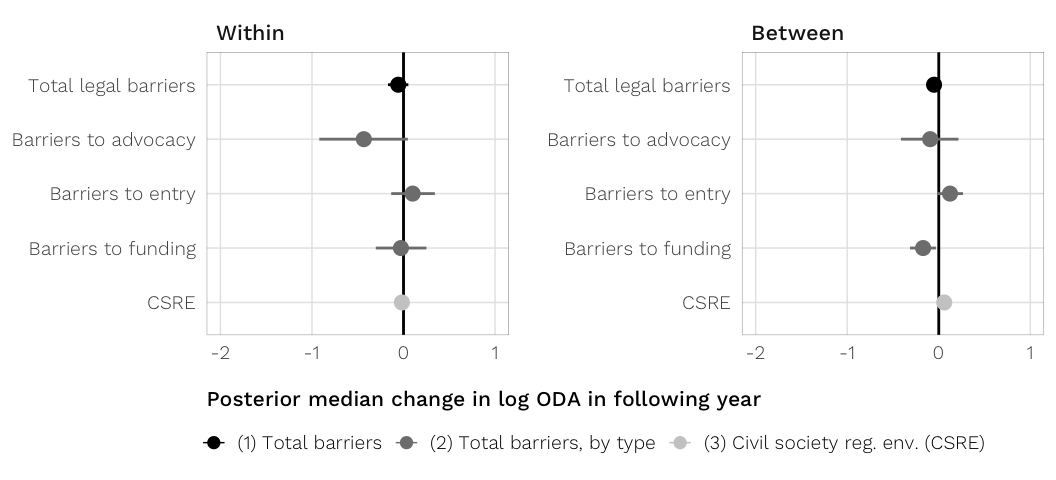
Complete results in a table
caption <- "The effect of anti-NGO legislation on OECD overseas development assistance (ODA) in the following year (H~1~), full models. Each cell contains the parameter's posterior median, the 95% credible interval, and the probability that the parameter is greater than zero (in italics). {#tbl:h1-coefs}"
note <- c("Dependent variable log transformed.")
table.h1 <- bayesgazer(mods.h1.next_year.bayes,
                       caption = caption, note = note)

cat(table.h1)| (1) | (2) | (3) | |
|---|---|---|---|
| Fixed part | |||
| Total legal barrierswithin | -0.06 (-0.17, 0.05); 0.15 |
||
| Total legal barriersbetween | -0.05 (-0.13, 0.02); 0.09 |
||
| Barriers to advocacywithin | -0.43 (-0.92, 0.05); 0.04 |
||
| Barriers to advocacybetween | -0.09 (-0.41, 0.22); 0.28 |
||
| Barriers to entrywithin | 0.10 (-0.13, 0.34); 0.79 |
||
| Barriers to entrybetween | 0.12 (-0.02, 0.26); 0.96 |
||
| Barriers to fundingwithin | -0.03 (-0.30, 0.25); 0.42 |
||
| Barriers to fundingbetween | -0.17 (-0.31, -0.03); 0.01 |
||
| Civil society reg. env. (CSRE)within | -0.02 (-0.09, 0.06); 0.33 |
||
| Civil society reg. env. (CSRE)between | 0.06 (-0.01, 0.13); 0.95 |
||
| Polity IV (0–10)within | -0.06 (-0.11, -0.00); 0.02 |
-0.06 (-0.12, -0.00); 0.02 |
-0.04 (-0.11, 0.03); 0.14 |
| Polity IV (0–10)between | 0.01 (-0.03, 0.05); 0.69 |
0.01 (-0.04, 0.05); 0.60 |
-0.02 (-0.08, 0.04); 0.27 |
| GDP per capita (log)within | -0.41 (-0.75, -0.14); 0.01 |
-0.42 (-0.75, -0.16); 0.01 |
-0.42 (-0.76, -0.15); 0.01 |
| GDP per capita (log)between | -0.18 (-0.26, -0.10); 0.00 |
-0.17 (-0.25, -0.09); 0.00 |
-0.18 (-0.26, -0.10); 0.00 |
| Trade as % of GDPwithin | -0.00 (-0.01, 0.00); 0.04 |
-0.00 (-0.01, 0.00); 0.04 |
-0.00 (-0.01, 0.00); 0.04 |
| Trade as % of GDPbetween | -0.00 (-0.00, 0.00); 0.05 |
-0.00 (-0.00, 0.00); 0.05 |
-0.00 (-0.00, 0.00); 0.08 |
| Corruptionwithin | 0.05 (-0.04, 0.14); 0.88 |
0.05 (-0.04, 0.14); 0.89 |
0.05 (-0.04, 0.14); 0.89 |
| Corruptionbetween | 0.05 (0.00, 0.10); 0.98 |
0.05 (0.00, 0.09); 0.98 |
0.05 (0.01, 0.10); 0.99 |
| Total aid in present year (log) | 0.87 (0.85, 0.88); 1.00 |
0.86 (0.85, 0.88); 1.00 |
0.87 (0.85, 0.88); 1.00 |
| Internal conflict in last 5 years | 0.08 (-0.12, 0.28); 0.78 |
0.07 (-0.13, 0.27); 0.75 |
0.11 (-0.09, 0.31); 0.86 |
| Natural disasters | 0.04 (0.01, 0.06); 0.99 |
0.03 (0.01, 0.06); 0.99 |
0.03 (0.01, 0.06); 0.99 |
| After 1989 | 0.58 (0.26, 0.88); 1.00 |
0.60 (0.30, 0.90); 1.00 |
0.56 (0.23, 0.86); 1.00 |
| Constant | 3.17 (2.26, 4.07); 1.00 |
3.07 (2.18, 3.95); 1.00 |
3.15 (2.26, 4.03); 1.00 |
| Random part | |||
| Within-country variability | 0.09 | 0.09 | 0.08 |
| Within-year variability | 0.26 | 0.26 | 0.28 |
| Residual random error | 2.69 | 2.69 | 2.69 |
| Model details | |||
| Imputed datasets (m) | 5 | 5 | 5 |
| N | 4480 | 4480 | 4480 |
| Posterior sample size | 4000 | 4000 | 4000 |
| Notes | |||
| Dependent variable log transformed. |
Complete results (nonimputed)
# The scaling factors are all the same across the three models, since they use
# the same dataset, so we only need scales_h1.1
scales.h1.next_year.no.imp <- mods.h1.next_year.raw.bayes %>%
  filter(m == "original") %>%
  select(m, starts_with("scales")) %>%
  pull(scales_h1.1) %>% .[[1]]

# Get model details and parameters
mods.h1.next_year.bayes.no.imp <- mods.h1.next_year.raw.bayes %>%
  select(-contains("scales")) %>%
  filter(m == "original") %>%
  gather(model.name, model, -m) %>%
  mutate(glance = model %>% map(glance),
         tidy = model %>% map(tidy, effects = "fixed")) %>%
  mutate(model_scale = model %>% map(add_scalemcmc))

h1_coefs <- mods.h1.next_year.bayes.no.imp %>%
  unnest(tidy) %>%
  filter(!duplicated(term, fromLast = TRUE)) %>%
  mutate(term_join = str_replace(term, "TRUE", "")) %>%
  left_join(coef.names.all, by = c("term_join" = "term")) %>%
  filter(term != "Intercept")

h1_coefs_named <- h1_coefs %>% pull(term) %>%
  set_names(h1_coefs$term_clean)

huxreg(mods.h1.next_year.bayes.no.imp$model_scale,
       coefs = c(h1_coefs_named, Constant = "Intercept"),
       stars = NULL, statistics = c(N = "nobs"),
       # ALL OTHER MCMC objects use conf.level to determine confidence level,
       # but brms uses prob for mysterious reasons
       tidy_args = list(conf.int = TRUE, prob = 0.95,
                        effects = "fixed", scalings = scales.h1.next_year.no.imp),
error_format = "({conf.low}, {conf.high})")| (1) | (2) | (3) | |
| Total legal barriers~within~ | 0.008 | ||
| (-0.095, 0.112) | |||
| Total legal barriers~between~ | -0.004 | ||
| (-0.097, 0.093) | |||
| Barriers to advocacy~within~ | -0.143 | ||
| (-0.579, 0.300) | |||
| Barriers to advocacy~between~ | -0.073 | ||
| (-0.493, 0.342) | |||
| Barriers to entry~within~ | 0.221 | ||
| (0.008, 0.440) | |||
| Barriers to entry~between~ | 0.009 | ||
| (-0.175, 0.187) | |||
| Barriers to funding~within~ | -0.117 | ||
| (-0.371, 0.130) | |||
| Barriers to funding~between~ | 0.012 | ||
| (-0.184, 0.213) | |||
| Civil society reg. env. (CSRE)~within~ | 0.117 | ||
| (0.039, 0.198) | |||
| Civil society reg. env. (CSRE)~between~ | -0.015 | ||
| (-0.110, 0.080) | |||
| Polity IV (0–10)~within~ | 0.056 | 0.053 | -0.016 |
| (0.002, 0.109) | (0.001, 0.104) | (-0.086, 0.054) | |
| Polity IV (0–10)~between~ | 0.045 | 0.046 | 0.059 |
| (-0.005, 0.095) | (-0.007, 0.095) | (-0.027, 0.139) | |
| GDP per capita (log)~within~ | -0.290 | -0.273 | -0.277 |
| (-0.621, 0.033) | (-0.591, 0.046) | (-0.600, 0.048) | |
| GDP per capita (log)~between~ | -0.273 | -0.272 | -0.275 |
| (-0.376, -0.171) | (-0.373, -0.169) | (-0.375, -0.176) | |
| Trade as % of GDP~within~ | -0.004 | -0.003 | -0.004 |
| (-0.007, 0.000) | (-0.007, 0.000) | (-0.008, 0.000) | |
| Trade as % of GDP~between~ | -0.002 | -0.002 | -0.002 |
| (-0.005, 0.001) | (-0.005, 0.001) | (-0.005, 0.000) | |
| Corruption~within~ | 0.144 | 0.146 | 0.147 |
| (0.060, 0.231) | (0.057, 0.232) | (0.061, 0.232) | |
| Corruption~between~ | 0.122 | 0.123 | 0.125 |
| (0.065, 0.181) | (0.065, 0.180) | (0.070, 0.183) | |
| Total aid in present year (log) | 0.745 | 0.744 | 0.739 |
| (0.723, 0.768) | (0.722, 0.768) | (0.716, 0.761) | |
| Internal conflict in last 5 years | -0.051 | -0.052 | -0.033 |
| (-0.252, 0.151) | (-0.261, 0.163) | (-0.245, 0.172) | |
| Natural disasters | 0.049 | 0.047 | 0.045 |
| (0.018, 0.079) | (0.015, 0.079) | (0.014, 0.076) | |
| After 1989 | -0.059 | -0.062 | -0.198 |
| (-0.416, 0.290) | (-0.419, 0.295) | (-0.577, 0.162) | |
| Constant | 6.177 | 6.172 | 6.345 |
| (5.010, 7.399) | (5.030, 7.331) | (5.169, 7.507) | |
| N | 4067 | 4067 | 4067 |
| . | |||
Model diagnostics
Country intercepts vary with an SD of 0.09 (etc.), year intercepts vary with an SD of 0.26 (etc.), and the SD of error not accounted for by either within-country or within-year variability is 2.69 (etc.)
Predicted ODA
Here, for the sake of computational efficiency and speed, we only use one of the imputed datasets for predictions. Technically we should base the predictions on all the merged chains, but (1) there’s no function that can handle that, (2) it would take forever to run predictions on each individual imputation and then combine the predictions, and (3) these are posterior medians anyway from ostensibly the same-ish distribution—quintupling the number of chains to simulate is overkill for drawing a picture.
model <- mods.h1.next_year.bayes %>%
  filter(m == "imp1", model.name == "mod.h1.barriers.total") %>%
  pull(model) %>% .[[1]]

# For whatever reason, stanreg objects return the full data frame used in the
# model, not just the model matrix, when calling object$data. model.frame()
# chokes on object$formula because of (1 | x) grouping terms, but
# get_all_vars() works.
new.data <- get_all_vars(model$formula, data = model$data) %>%
  select(-c(barriers.total_within, year, cowcode)) %>%
  summarise_all(typical) %>%
  mutate(id = 1) %>%
  right_join(expand.grid(barriers.total_within = seq(-3, 4, 0.5),
                         cowcode = 1000:1049,
                         year = 1981:2012,
                         id = 1), by = "id") %>% select(-id)

predicted.h1.barriers.total <- new.data %>%
  nest(-cowcode) %>%
  mutate(predicted = future_map(.x = data, ~ generate_predictions(.x))) %>%
  unnest()

df.plot.data.h1 <- predicted.h1.barriers.total %>%
  group_by(cowcode, barriers.total_within) %>%
  summarise_at(vars(predicted), funs(mean(.))) %>%
  ungroup()

df.plot.data.mean.h1 <- df.plot.data.h1 %>%
  group_by(barriers.total_within) %>%
  summarise(predicted = mean(predicted)) %>%
  mutate(cowcode = 1)  # Fake country so the line plots
barriers.indiv.clean.names <- tribble(
~barrier, ~barrier.clean,
"advocacy_within", "Barriers to advocacy",
"entry_within", "Barriers to entry",
"funding_within", "Barriers to funding"
)
model <- mods.h1.next_year.bayes %>%
filter(m == "imp1", model.name == "mod.h1.type.total") %>%
select(model) %>% .[[1]] %>% .[[1]]
hypothetical.bounds <- get_all_vars(model$formula, data = model$data) %>%
select(advocacy_within, entry_within, funding_within) %>%
summarise_all(funs(min, max)) %>%
gather(key, value) %>%
mutate(value = round(value, 0)) %>%
# Have to separate on _m because of multiple _s, then re-add the m
separate(key, into = c("term", "variable"), sep = "_m") %>%
mutate(variable = paste0("m", variable)) %>%
spread(variable, value)
new.data.hypothetical.nested <- hypothetical.bounds %>%
nest(-term) %>%
mutate(newdata = map2(.x = data, .y = term,
~ expand.grid(term = seq(.x$min, .x$max, by = 0.5),
cowcode = 1000:1049,
year = 1981:2012,
id = 1) %>%
# Rename the term column to the actual term name
magrittr::set_colnames(c(.y, colnames(.)[-1]))))
new.data.hypothetical <- as_tibble(bind_rows(new.data.hypothetical.nested$newdata)) %>%
mutate_at(vars(contains("within")), funs(ifelse(is.na(.), 0, .)))
new.data <- get_all_vars(model$formula, data = model$data) %>%
select(-c(advocacy_within, entry_within, funding_within, year, cowcode)) %>%
summarise_all(typical) %>%
mutate(id = 1) %>%
right_join(new.data.hypothetical, by = "id") %>% select(-id)
predicted.h1.barriers.individual <- new.data %>%
nest(-cowcode) %>%
mutate(predicted = future_map(.x = data, ~ generate_predictions(.x))) %>%
unnest()
df.plot.data.indiv.h1 <- predicted.h1.barriers.individual %>%
gather(barrier, barrier.value, c(advocacy_within, entry_within, funding_within)) %>%
group_by(cowcode, barrier.value, barrier) %>%
summarise_at(vars(predicted), funs(mean(.))) %>%
left_join(barriers.indiv.clean.names, by = "barrier")
df.plot.data.mean.indiv.h1 <- df.plot.data.indiv.h1 %>%
group_by(barrier, barrier.value) %>%
summarise(predicted = mean(predicted)) %>%
mutate(cowcode = 1) %>% # Fake country so the line plots
left_join(barriers.indiv.clean.names, by = "barrier")# Combine the two plot data frames
df.plot.data.both.h1 <- df.plot.data.h1 %>%
mutate(barrier = "barriers.total_within", barrier.clean = "Total barriers") %>%
rename(barrier.value = barriers.total_within) %>%
bind_rows(df.plot.data.indiv.h1) %>%
mutate(barrier.clean = ordered(fct_inorder(barrier.clean)),
highlight = ifelse(barrier.clean == "Total barriers", TRUE, FALSE))
df.plot.data.mean.both.h1 <- df.plot.data.mean.h1 %>%
mutate(barrier = "barriers.total_within", barrier.clean = "Total barriers") %>%
rename(barrier.value = barriers.total_within) %>%
bind_rows(df.plot.data.mean.indiv.h1) %>%
mutate(barrier.clean = ordered(fct_inorder(barrier.clean)))
# Create data frame for highlighting the total panel
df.panel.highlight.h1 <- df.plot.data.both.h1 %>%
distinct(barrier.clean, highlight)
fig.predicted.h1.barriers.both <- ggplot(df.plot.data.both.h1,
aes(x = barrier.value, y = expm1(predicted),
group = cowcode)) +
geom_rect(data = df.panel.highlight.h1, aes(fill = highlight), inherit.aes = FALSE,
xmin = -Inf, xmax = Inf, ymin = -Inf, ymax = Inf, alpha = 0.15) +
geom_vline(xintercept = 0, colour = "black", size = 0.5) +
geom_smooth(method = "lm", size = 0.1, alpha = 0.1,
colour = simulation.individual) +
geom_smooth(data = df.plot.data.mean.both.h1, size = 1.5,
method = "lm", colour = simulation.mean) +
labs(x = "Difference from average number of anti-NGO barriers in country (within effects)",
y = "Predicted ODA in the following year") +
scale_y_continuous(labels = dollar, trans = log1p_trans()) +
scale_fill_manual(values = c(NA, "grey50"), guide = FALSE) +
facet_wrap(~ barrier.clean, scales = "free_x") +
theme_donors() +
theme(axis.title.x = element_text(hjust = 0))
fig.predicted.h1.barriers.both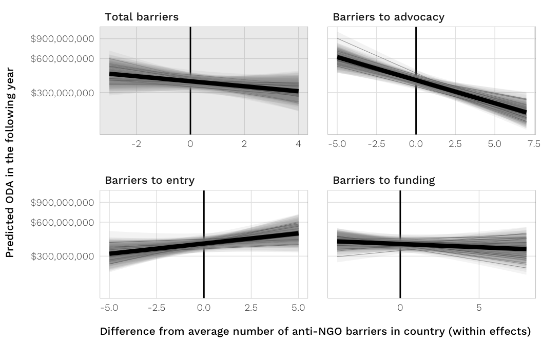
fig.save.cairo(fig.predicted.h1.barriers.both, filename = "fig-predicted-h1",
width = 5.5, height = 3.5)H2: Donors shift aid to tamer causes
H2: As restrictive laws against NGOs are enacted, donors start increasing funds for ‘tamer’ causes, and decreasing funds for politically sensitive causes.
Our dependent variable for this hypothesis is the percentage of ODA (still in constant 2011 dollars) allocated for contentious purposes, again leaded by one year. We classify contentious aid as any project focused on government and civil society (DAC codes 150 and 151) or conflict prevention and resolution, peace and security (DAC code 152).
Working with proportion data, however, poses interesting mathematical and methodological challenges, since the range of possible outcomes is limited to a value between 0 and 1. Treating proportion variables in a mixed model is technically possible, but it yields predicitions that go beyond the allowable range of values (1.13, -0.5, etc.). Treating the proportion as a binomial variable is also possible and is indeed one of the ways to use the glm() function in R. However, this entails considering the proportion as a ratio of success and failures. In this case, treating a dollar of contentious aid as a success feels off, especially since aid amounts aren’t independent events—it’s not like each dollar of aid goes through a probabalistic process like a coin flip.
One recommendation by Ben Bolker, the maintainer of lme4, is to use a logit transformation of the dependent variable in lmer() models. This seems to be standard practice in political science research, too. Logit transformations still can’t handle values of exactly 0 or 1, though, so we winsorize those values by adding or subtracting 0.001 to the extremes.
Another solution is to use beta regression, which constrains the outcome variable to values between 0 and 1, but unfortunately does not allow for values of exactly 0 or 1. Zero-and-one inflated beta regression models, however, make adjustments for this, and we include a set of these models as a robustness check. We stick with logit-linear models, though, since we want to compare the ratio of contentious aid to non-contentious aid (rather than the percent of contentious aid) and keep the comparison parallel with our H3 models, which only compare the ratio of aid channeled through all NGOs.
We thus use a logit-linear model of the ratio of contentious aid to non-contentious aid:
\[ln( \frac{\text{contentious ODA}_{\text{OECD}}}{\text{noncontentious ODA}_{\text{OECD}}} )_{i, t+1} = \text{NGO legislation}_{it} + \text{controls}_{it}\]
We look at NGO legislation in the same ways as H1 and use the same controls.
# Get scaling factors
scales.h2.next_year <- mods.h2.next_year.raw.bayes %>%
  filter(m != "original") %>%
  select(m, starts_with("scales")) %>%
  gather(scales.name, scales, -m)

# Get model details and parameters
mods.h2.next_year.bayes <- mods.h2.next_year.raw.bayes %>%
  filter(m != "original") %>%
  select(m, starts_with("mod")) %>%
  gather(model.name, model, -m) %>%
  mutate(glance = model %>% map(glance),
         tidy = model %>% map(tidy)) %>%
  bind_cols(select(scales.h2.next_year, -m))
MCMC diagnostics
Check fit
Again, use one of the imputed models (mod.h2.barriers.total) to check for fit and convergence.
model.to.check <- mods.h2.next_year.bayes %>%
  filter(m == "imp1", model.name == "mod.h2.barriers.total") %>%
  select(model) %>% .[[1]] %>% .[[1]]
Posterior predictive distribution vs. observed outcome?
Check convergence
Chain convergence:
Results
Coefficients
vars.to.plot <- c("barriers.total_within", "barriers.total_between",
                  "advocacy_within", "advocacy_between",
                  "entry_within", "entry_between",
                  "funding_within", "funding_between",
                  "csre_within", "csre_between")

mods.h2.melded <- bayes.meld(mods.h2.next_year.bayes,
                             vars.to.plot, exponentiate = TRUE)$melded.summary

plot.data <- mods.h2.melded %>%
  left_join(coef.names.all, by = "term") %>%
  left_join(model.names, by = c("model.name" = "model")) %>%
  mutate(term = factor(term, levels = vars.to.plot, ordered = TRUE)) %>%
  arrange(desc(term)) %>%
  mutate(term_plot = ordered(fct_inorder(term_plot_short))) %>%
  mutate(coef.type = case_when(
    str_detect(.$term, "_within") ~ "Within",
    str_detect(.$term, "_between") ~ "Between",
  )) %>%
  mutate(coef.type = factor(coef.type, levels = c("Within", "Between"),
                            ordered = TRUE)) %>%
  mutate(model_clean = factor(model_clean, levels = rev(unique(model_clean)), ordered = TRUE))

fig.coefs.h2 <- ggplot(plot.data, aes(x = med, y = term_plot, colour = model_clean)) +
  geom_vline(xintercept = 1, colour = "black", size = 0.5) +
  geom_pointrangeh(aes(xmin = `2.5%`, xmax = `97.5%`), size = 0.5, fatten = 3) +
  labs(x = "Percent change in ratio of contentious aid (odds ratio)", y = NULL) +
  scale_colour_manual(values = model.colors, name = NULL) +
  expand_limits(x = c(0.6, 1.3)) +
  guides(color = guide_legend(override.aes = list(size = 0.25))) +
  theme_donors() +
  theme(legend.justification = "left",
        legend.box.margin = margin(l = -0.75, t = -0.5, unit = "lines"),
        axis.title.x = element_text(hjust = 0)) +
  facet_wrap(~ coef.type, scales = "free", ncol = 2)
fig.coefs.h2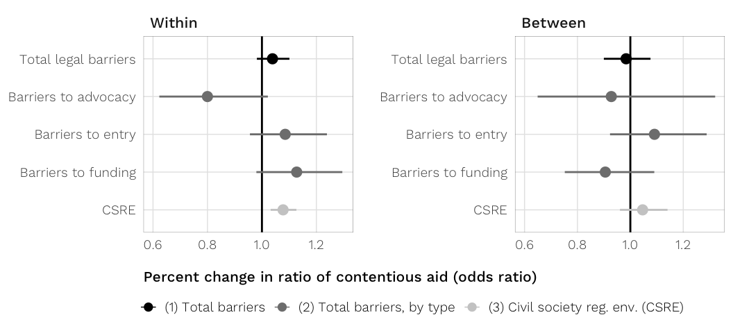
Complete results in a table
caption <- "The effect of anti-NGO legislation on the proportion of OECD overseas development assistance (ODA) committed to contentious purposes in the following year (H~2~), full models. Each cell contains the parameter's posterior median, the 95% credible interval, and the probability that the parameter is greater than one (in italics). {#tbl:h2-coefs}"
note <- c("Logit-linear models. Percent change odds ratios reported.")

table.h2 <- bayesgazer(mods.h2.next_year.bayes, exponentiate = TRUE,
                       caption = caption, note = note)

cat(table.h2)| (1) | (2) | (3) | |
|---|---|---|---|
| Fixed part (odds ratios) | |||
| Total legal barrierswithin | 1.04 (0.98, 1.10); 0.90 |
||
| Total legal barriersbetween | 0.98 (0.90, 1.08); 0.36 |
||
| Barriers to advocacywithin | 0.80 (0.62, 1.02); 0.04 |
||
| Barriers to advocacybetween | 0.93 (0.65, 1.32); 0.34 |
||
| Barriers to entrywithin | 1.09 (0.96, 1.24); 0.90 |
||
| Barriers to entrybetween | 1.09 (0.92, 1.29); 0.85 |
||
| Barriers to fundingwithin | 1.13 (0.98, 1.30); 0.95 |
||
| Barriers to fundingbetween | 0.91 (0.75, 1.09); 0.14 |
||
| Civil society reg. env. (CSRE)within | 1.08 (1.03, 1.13); 1.00 |
||
| Civil society reg. env. (CSRE)between | 1.05 (0.96, 1.14); 0.85 |
||
| Polity IV (0–10)within | 1.03 (1.00, 1.06); 0.97 |
1.03 (1.00, 1.06); 0.97 |
0.99 (0.95, 1.03); 0.25 |
| Polity IV (0–10)between | 1.09 (1.04, 1.14); 1.00 |
1.08 (1.03, 1.13); 1.00 |
1.06 (0.98, 1.14); 0.92 |
| GDP per capita (log)within | 0.97 (0.81, 1.16); 0.36 |
0.96 (0.80, 1.15); 0.34 |
0.99 (0.82, 1.18); 0.45 |
| GDP per capita (log)between | 0.71 (0.64, 0.77); 0.00 |
0.71 (0.65, 0.78); 0.00 |
0.71 (0.64, 0.77); 0.00 |
| Trade as % of GDPwithin | 1.00 (1.00, 1.00); 0.04 |
1.00 (1.00, 1.00); 0.05 |
1.00 (1.00, 1.00); 0.03 |
| Trade as % of GDPbetween | 1.00 (1.00, 1.00); 0.95 |
1.00 (1.00, 1.00); 0.95 |
1.00 (1.00, 1.00); 0.95 |
| Corruptionwithin | 1.05 (1.00, 1.10); 0.98 |
1.05 (1.00, 1.11); 0.98 |
1.06 (1.01, 1.11); 0.99 |
| Corruptionbetween | 1.07 (1.01, 1.13); 0.99 |
1.06 (1.01, 1.12); 0.99 |
1.07 (1.02, 1.13); 1.00 |
| Proportion of contentious aid in present year (logit) | 1.28 (1.24, 1.32); 1.00 |
1.28 (1.24, 1.32); 1.00 |
1.27 (1.23, 1.31); 1.00 |
| Internal conflict in last 5 years | 1.07 (0.94, 1.21); 0.84 |
1.06 (0.93, 1.20); 0.80 |
1.09 (0.96, 1.24); 0.91 |
| Natural disasters | 0.99 (0.97, 1.01); 0.22 |
0.99 (0.97, 1.01); 0.22 |
0.99 (0.97, 1.01); 0.16 |
| After 1989 | 4.61 (3.02, 7.05); 1.00 |
4.69 (3.08, 7.22); 1.00 |
4.34 (2.87, 6.72); 1.00 |
| Constant | 0.09 (0.03, 0.25); 0.00 |
0.08 (0.03, 0.23); 0.00 |
0.10 (0.04, 0.27); 0.00 |
| Random part (original coefficients) | |||
| Within-country variability | 0.50 | 0.50 | 0.50 |
| Within-year variability | 0.52 | 0.52 | 0.52 |
| Residual random error | 1.33 | 1.33 | 1.33 |
| Model details | |||
| Imputed datasets (m) | 5 | 5 | 5 |
| N | 3922 | 3922 | 3922 |
| Posterior sample size | 4000 | 4000 | 4000 |
| Notes | |||
| Logit-linear models. Percent change odds ratios reported. |
Complete results (nonimputed)
# The scaling factors are all the same across the three models, since they use
# the same dataset, so we only need scales_h1.1
scales.h2.next_year.no.imp <- mods.h2.next_year.raw.bayes %>%
  filter(m == "original") %>%
  select(m, starts_with("scales")) %>%
  pull(scales_h2.1) %>% .[[1]]

# Get model details and parameters
mods.h2.next_year.bayes.no.imp <- mods.h2.next_year.raw.bayes %>%
  select(-contains("scales")) %>%
  filter(m == "original") %>%
  gather(model.name, model, -m) %>%
  mutate(glance = model %>% map(glance),
         tidy = model %>% map(tidy, effects = "fixed")) %>%
  mutate(model_scale = model %>% map(add_scalemcmc))

h2_coefs <- mods.h2.next_year.bayes.no.imp %>%
  unnest(tidy) %>%
  filter(!duplicated(term, fromLast = TRUE)) %>%
  mutate(term_join = str_replace(term, "TRUE", "")) %>%
  left_join(coef.names.all, by = c("term_join" = "term")) %>%
  filter(term != "Intercept")

h2_coefs_named <- h2_coefs %>% pull(term) %>%
  set_names(h2_coefs$term_clean)

huxreg(mods.h2.next_year.bayes.no.imp$model_scale,
       coefs = c(h2_coefs_named, Constant = "Intercept"),
       stars = NULL, statistics = c(N = "nobs"),
       tidy_args = list(conf.int = TRUE, prob = 0.95, exponentiate = TRUE,
                        effects = "fixed", scalings = scales.h2.next_year.no.imp),
error_format = "({conf.low}, {conf.high})")| (1) | (2) | (3) | |
| Total legal barriers~within~ | 1.060 | ||
| (0.999, 1.121) | |||
| Total legal barriers~between~ | 1.005 | ||
| (0.923, 1.093) | |||
| Barriers to advocacy~within~ | 0.873 | ||
| (0.672, 1.135) | |||
| Barriers to advocacy~between~ | 1.082 | ||
| (0.759, 1.546) | |||
| Barriers to entry~within~ | 1.080 | ||
| (0.953, 1.230) | |||
| Barriers to entry~between~ | 1.092 | ||
| (0.935, 1.278) | |||
| Barriers to funding~within~ | 1.134 | ||
| (0.981, 1.309) | |||
| Barriers to funding~between~ | 0.899 | ||
| (0.748, 1.075) | |||
| Civil society reg. env. (CSRE)~within~ | 1.081 | ||
| (1.034, 1.131) | |||
| Civil society reg. env. (CSRE)~between~ | 1.041 | ||
| (0.956, 1.133) | |||
| Polity IV (0–10)~within~ | 1.033 | 1.031 | 0.984 |
| (1.001, 1.067) | (1.001, 1.063) | (0.945, 1.023) | |
| Polity IV (0–10)~between~ | 1.091 | 1.089 | 1.058 |
| (1.041, 1.141) | (1.040, 1.141) | (0.982, 1.137) | |
| GDP per capita (log)~within~ | 0.948 | 0.944 | 0.978 |
| (0.788, 1.143) | (0.787, 1.130) | (0.810, 1.178) | |
| GDP per capita (log)~between~ | 0.704 | 0.705 | 0.705 |
| (0.643, 0.768) | (0.646, 0.770) | (0.644, 0.770) | |
| Trade as % of GDP~within~ | 0.998 | 0.998 | 0.998 |
| (0.996, 1.000) | (0.996, 1.000) | (0.996, 1.000) | |
| Trade as % of GDP~between~ | 1.003 | 1.003 | 1.003 |
| (1.000, 1.005) | (1.000, 1.005) | (1.000, 1.005) | |
| Corruption~within~ | 1.040 | 1.041 | 1.048 |
| (0.987, 1.095) | (0.990, 1.095) | (0.996, 1.104) | |
| Corruption~between~ | 1.064 | 1.062 | 1.066 |
| (1.010, 1.117) | (1.010, 1.116) | (1.014, 1.118) | |
| Proportion of contentious aid in present year (logit) | 1.271 | 1.269 | 1.267 |
| (1.231, 1.311) | (1.229, 1.311) | (1.226, 1.310) | |
| Internal conflict in last 5 years | 1.069 | 1.064 | 1.091 |
| (0.938, 1.211) | (0.938, 1.202) | (0.964, 1.240) | |
| Natural disasters | 0.992 | 0.991 | 0.989 |
| (0.972, 1.013) | (0.970, 1.011) | (0.970, 1.010) | |
| After 1989 | 4.729 | 4.758 | 4.520 |
| (3.103, 7.250) | (3.088, 7.332) | (2.908, 7.033) | |
| Constant | 0.084 | 0.077 | 0.095 |
| (0.031, 0.229) | (0.029, 0.198) | (0.037, 0.239) | |
| N | 3826 | 3826 | 3826 |
| . | |||
Predicted proportion of contentious aid
model <- mods.h2.next_year.bayes %>%
  filter(m == "imp1", model.name == "mod.h2.barriers.total") %>%
  select(model) %>% .[[1]] %>% .[[1]]

new.data <- get_all_vars(model$formula, data = model$data) %>%
  select(-c(barriers.total_within, year, cowcode)) %>%
  summarise_all(typical) %>%
  mutate(id = 1) %>%
  right_join(expand.grid(barriers.total_within = seq(-3, 4, 0.5),
                         cowcode = 1000:1049,
                         year = 1981:2012,
                         id = 1), by = "id") %>% select(-id)

predicted.h2.barriers.total <- new.data %>%
  nest(-cowcode) %>%
  mutate(predicted = future_map(.x = data, ~ generate_predictions(.x))) %>%
  unnest()

df.plot.data.h2 <- predicted.h2.barriers.total %>%
  group_by(cowcode, barriers.total_within) %>%
  summarise_at(vars(predicted), funs(mean(.))) %>%
  ungroup() %>%
  mutate(value.fixed = inv.logit(predicted, a = 0.001))

df.plot.data.mean.h2 <- df.plot.data.h2 %>%
  group_by(barriers.total_within) %>%
  summarise(predicted = mean(predicted)) %>%
  mutate(value.fixed = inv.logit(predicted, a = 0.001)) %>%
  mutate(cowcode = 1)  # Fake country so the line plots
barriers.indiv.clean.names <- tribble(
~barrier, ~barrier.clean,
"advocacy_within", "Barriers to advocacy",
"entry_within", "Barriers to entry",
"funding_within", "Barriers to funding"
)
model <- mods.h2.next_year.bayes %>%
filter(m == "imp1", model.name == "mod.h2.type.total") %>%
select(model) %>% .[[1]] %>% .[[1]]
hypothetical.bounds <- get_all_vars(model$formula, data = model$data) %>%
select(advocacy_within, entry_within, funding_within) %>%
summarise_all(funs(min, max)) %>%
gather(key, value) %>%
mutate(value = round(value, 0)) %>%
# Have to separate on _m because of multiple _s, then re-add the m
separate(key, into = c("term", "variable"), sep = "_m") %>%
mutate(variable = paste0("m", variable)) %>%
spread(variable, value)
new.data.hypothetical.nested <- hypothetical.bounds %>%
nest(-term) %>%
mutate(newdata = map2(.x = data, .y = term,
~ expand.grid(term = seq(.x$min, .x$max, by = 0.5),
cowcode = 1000:1049,
year = 1981:2012,
id = 1) %>%
# Rename the term column to the actual term name
magrittr::set_colnames(c(.y, colnames(.)[-1]))))
new.data.hypothetical <- as_tibble(bind_rows(new.data.hypothetical.nested$newdata)) %>%
mutate_at(vars(contains("within")), funs(ifelse(is.na(.), 0, .)))
new.data <- get_all_vars(model$formula, data = model$data) %>%
select(-c(advocacy_within, entry_within, funding_within, year, cowcode)) %>%
summarise_all(typical) %>%
mutate(id = 1) %>%
right_join(new.data.hypothetical, by = "id") %>% select(-id)
predicted.h2.barriers.individual <- new.data %>%
nest(-cowcode) %>%
mutate(predicted = future_map(.x = data, ~ generate_predictions(.x))) %>%
unnest()
df.plot.data.indiv.h2 <- predicted.h2.barriers.individual %>%
gather(barrier, barrier.value, c(advocacy_within, entry_within, funding_within)) %>%
group_by(cowcode, barrier.value, barrier) %>%
summarise_at(vars(predicted), funs(mean(.))) %>%
mutate(value.fixed = inv.logit(predicted, a = 0.001)) %>%
left_join(barriers.indiv.clean.names, by = "barrier")
df.plot.data.mean.indiv.h2 <- df.plot.data.indiv.h2 %>%
group_by(barrier, barrier.value) %>%
summarise(predicted = mean(predicted)) %>%
mutate(cowcode = 1) %>% # Fake country so the line plots
mutate(value.fixed = inv.logit(predicted, a = 0.001)) %>%
left_join(barriers.indiv.clean.names, by = "barrier")# Combine the two plot data frames
df.plot.data.both.h2 <- df.plot.data.h2 %>%
mutate(barrier = "barriers.total_within", barrier.clean = "Total barriers") %>%
rename(barrier.value = barriers.total_within) %>%
bind_rows(df.plot.data.indiv.h2) %>%
mutate(barrier.clean = ordered(fct_inorder(barrier.clean)),
highlight = ifelse(barrier.clean == "Total barriers", TRUE, FALSE))
df.plot.data.mean.both.h2 <- df.plot.data.mean.h2 %>%
mutate(barrier = "barriers.total_within", barrier.clean = "Total barriers") %>%
rename(barrier.value = barriers.total_within) %>%
bind_rows(df.plot.data.mean.indiv.h2) %>%
mutate(barrier.clean = ordered(fct_inorder(barrier.clean)))
# Create data frame for highlighting the total panel
df.panel.highlight.h2 <- df.plot.data.both.h2 %>%
distinct(barrier.clean, highlight)
fig.predicted.h2.barriers.both <- ggplot(df.plot.data.both.h2,
aes(x = barrier.value,
y = value.fixed, group = cowcode)) +
geom_rect(data = df.panel.highlight.h2, aes(fill = highlight), inherit.aes = FALSE,
xmin = -Inf, xmax = Inf, ymin = -Inf, ymax = Inf, alpha = 0.15) +
geom_vline(xintercept = 0, colour = "black", size = 0.5) +
geom_smooth(method = "lm", size = 0.1, alpha = 0.1, colour = simulation.individual) +
geom_smooth(data = df.plot.data.mean.both.h2, size = 1.5,
method = "lm", colour = simulation.mean) +
labs(x = "Difference from average level of NGO legislation in country (within effect)",
y = "Predicted proportion of\ncontentious aid in the following year") +
scale_y_continuous(labels = percent_format(accuracy = 1)) +
scale_fill_manual(values = c(NA, "grey50"), guide = FALSE) +
facet_wrap(~ barrier.clean, scales = "free_x") +
theme_donors() +
theme(axis.title.x = element_text(hjust = 0))
fig.predicted.h2.barriers.both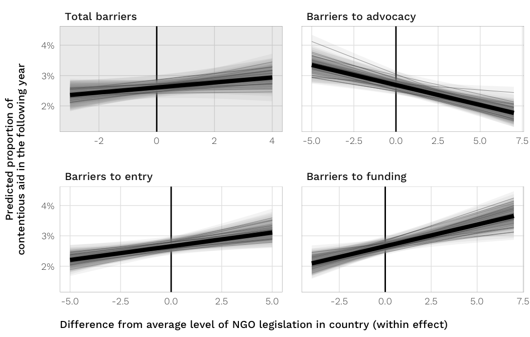
fig.save.cairo(fig.predicted.h2.barriers.both, filename = "fig-predicted-h2",
width = 5.5, height = 3.5)H3: Donors shift aid to international NGOs
H3: As restrictive laws against local NGOs increase, states should be more likely to provide aid to INGOs rather than local NGOs.
We use two dependent variables for this hypothesis: the proportion of aid channeled through either (1) domestic or (2) international or US-based (or foreign) NGOs, once again leaded by one year. The OECD and AidData do not track the channels of aid delivery, so we cannot see how aid is distributed on a global scale. USAID, however, does track channels, so we can measure how much aid goes to domestic NGOs (and also US-based and international NGOs). USAID didn’t start tracking this until 2001, though, so we have to limit our models to 2001–2013. (Boo.)
It would be cool to model the ratio aid channeled through domestic to foreign NGOs, but doing that causes weird mathematical issues with logit transformations, since the ratios can exceed 1.
Because the DVs are proportions, we have to make the same assumptions and weird interpretive tricks as H2, building a logit-linear model of the ratio of domestic or foreign NGO aid to all other channels:
\[ln( \frac{\text{Aid to (domestic or foreign) NGOs}_{\text{USAID}}}{\text{Aid to other channels}_{\text{USAID}}} )_{i, t+1} = \text{NGO legislation}_{it} + \text{controls}_{it}\]
We also include zero-one-inflated beta regression models as robustness checks.
Again, we use the same NGO legislation variables as H1 and H2 and use the same controls, except we omit “After 1989” since no observations actually occur after 1989.
# Get scaling factors
scales.h3.dom.next_year <- mods.h3.dom.next_year.raw %>%
  filter(m != "original") %>%
  select(m, starts_with("scales")) %>%
  gather(scales.name, scales, -m)

# Get model details and parameters
mods.h3.dom.next_year.bayes <- mods.h3.dom.next_year.raw %>%
  filter(m != "original") %>%
  select(m, starts_with("mod")) %>%
  gather(model.name, model, -m) %>%
  mutate(glance = model %>% map(glance),
         tidy = model %>% map(tidy)) %>%
  bind_cols(select(scales.h3.dom.next_year, -m))
# Get scaling factors
scales.h3.foreign.next_year <- mods.h3.foreign.next_year.raw %>%
filter(m != "original") %>%
select(m, starts_with("scales")) %>%
gather(scales.name, scales, -m)
# Get model details and parameters
mods.h3.foreign.next_year.bayes <- mods.h3.foreign.next_year.raw %>%
filter(m != "original") %>%
select(m, starts_with("mod")) %>%
gather(model.name, model, -m) %>%
mutate(glance = model %>% map(glance),
tidy = model %>% map(tidy)) %>%
bind_cols(select(scales.h3.foreign.next_year, -m))MCMC diagnostics
Check fit
Again, use one of the imputed models (mod.h3.barriers.total) to check for fit and convergence.
model.to.check <- mods.h3.dom.next_year.bayes %>%
  filter(m == "imp1", model.name == "mod.h3.barriers.total") %>%
  select(model) %>% .[[1]] %>% .[[1]]
Posterior predictive distribution vs. observed outcome?
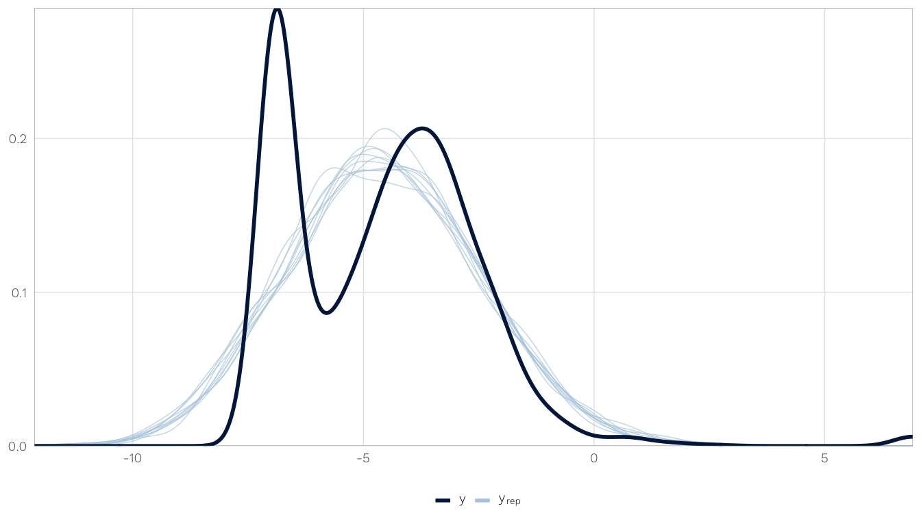
Check convergence
Chain convergence:
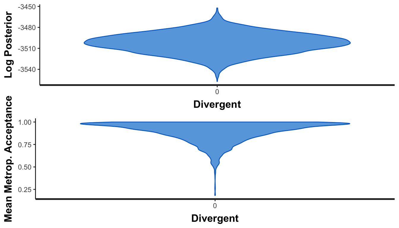
Results
Proportion to domestic NGOs
caption <- "The effect of anti-NGO legislation on the proportion of US aid channeled through *domestic* NGOs in the following year (H~3~), full models. Each cell contains the parameter's posterior median, the 95% credible interval, and the probability that the parameter is greater than one (in italics) {#tbl:h3-domestic-coefs}"
note <- c("Logit-linear models. Percent change odds ratios reported.")

table.h3.domestic <- bayesgazer(mods.h3.dom.next_year.bayes,
                                caption = caption, note = note, exponentiate = TRUE)

cat(table.h3.domestic)| (1) | (2) | (3) | |
|---|---|---|---|
| Fixed part (odds ratios) | |||
| Total legal barrierswithin | 1.15 (1.03, 1.29); 0.99 |
||
| Total legal barriersbetween | 1.04 (0.93, 1.16); 0.75 |
||
| Barriers to advocacywithin | 0.99 (0.56, 1.76); 0.49 |
||
| Barriers to advocacybetween | 1.10 (0.73, 1.67); 0.68 |
||
| Barriers to entrywithin | 1.01 (0.75, 1.35); 0.53 |
||
| Barriers to entrybetween | 1.14 (0.94, 1.39); 0.91 |
||
| Barriers to fundingwithin | 1.34 (1.01, 1.78); 0.98 |
||
| Barriers to fundingbetween | 0.92 (0.73, 1.16); 0.24 |
||
| Civil society reg. env. (CSRE)within | 0.92 (0.80, 1.07); 0.14 |
||
| Civil society reg. env. (CSRE)between | 1.04 (0.92, 1.18); 0.74 |
||
| Polity IV (0–10)within | 0.88 (0.79, 0.98); 0.01 |
0.88 (0.80, 0.98); 0.01 |
0.91 (0.80, 1.02); 0.06 |
| Polity IV (0–10)between | 1.01 (0.94, 1.08); 0.58 |
1.00 (0.94, 1.07); 0.53 |
0.96 (0.86, 1.07); 0.25 |
| GDP per capita (log)within | 1.89 (1.06, 3.27); 0.98 |
1.93 (1.08, 3.35); 0.99 |
2.01 (1.12, 3.49); 0.99 |
| GDP per capita (log)between | 1.04 (0.91, 1.20); 0.74 |
1.05 (0.91, 1.20); 0.75 |
1.05 (0.92, 1.21); 0.77 |
| Trade as % of GDPwithin | 1.00 (0.99, 1.01); 0.55 |
1.00 (0.99, 1.01); 0.55 |
1.00 (0.99, 1.01); 0.48 |
| Trade as % of GDPbetween | 1.00 (0.99, 1.00); 0.00 |
1.00 (0.99, 1.00); 0.01 |
0.99 (0.99, 1.00); 0.00 |
| Corruptionwithin | 1.19 (1.04, 1.41); 0.98 |
1.20 (1.05, 1.42); 0.99 |
1.18 (1.03, 1.39); 0.97 |
| Corruptionbetween | 1.15 (1.06, 1.24); 1.00 |
1.14 (1.05, 1.23); 1.00 |
1.14 (1.06, 1.23); 1.00 |
| Proportion of aid to domestic NGOs in present year (logit) | 1.39 (1.32, 1.46); 1.00 |
1.38 (1.31, 1.45); 1.00 |
1.39 (1.32, 1.46); 1.00 |
| Internal conflict in last 5 years | 1.23 (0.94, 1.59); 0.94 |
1.24 (0.95, 1.62); 0.95 |
1.22 (0.94, 1.59); 0.93 |
| Natural disasters | 0.99 (0.96, 1.02); 0.24 |
0.99 (0.96, 1.02); 0.21 |
0.99 (0.96, 1.02); 0.29 |
| Constant | 0.02 (0.00, 0.09); 0.00 |
0.02 (0.00, 0.08); 0.00 |
0.02 (0.01, 0.11); 0.00 |
| Random part (original coefficients) | |||
| Within-country variability | 0.72 | 0.73 | 0.71 |
| Within-year variability | 0.18 | 0.18 | 0.19 |
| Residual random error | 1.55 | 1.55 | 1.55 |
| Model details | |||
| Imputed datasets (m) | 5 | 5 | 5 |
| N | 1751 | 1751 | 1751 |
| Posterior sample size | 4000 | 4000 | 4000 |
| Notes | |||
| Logit-linear models. Percent change odds ratios reported. |
Proportion to foreign NGOs
caption <- "The effect of anti-NGO legislation on the proportion of US aid channeled through *US-based and international* NGOs in the following year (H~3~), full models. Each cell contains the parameter's posterior median, the 95% credible interval, and the probability that the parameter is greater than one (in italics) {#tbl:h3-foreign-coefs}"
note <- c("Logit-linear models. Percent change odds ratios reported.")

table.h3.domestic <- bayesgazer(mods.h3.foreign.next_year.bayes,
                                caption = caption, note = note, exponentiate = TRUE)

cat(table.h3.domestic)| (1) | (2) | (3) | |
|---|---|---|---|
| Fixed part (odds ratios) | |||
| Total legal barrierswithin | 0.95 (0.83, 1.08); 0.20 |
||
| Total legal barriersbetween | 1.02 (0.89, 1.16); 0.60 |
||
| Barriers to advocacywithin | 1.04 (0.53, 1.99); 0.54 |
||
| Barriers to advocacybetween | 0.96 (0.59, 1.54); 0.44 |
||
| Barriers to entrywithin | 1.36 (0.98, 1.90); 0.97 |
||
| Barriers to entrybetween | 1.07 (0.84, 1.35); 0.71 |
||
| Barriers to fundingwithin | 0.71 (0.52, 0.97); 0.01 |
||
| Barriers to fundingbetween | 0.99 (0.76, 1.30); 0.48 |
||
| Civil society reg. env. (CSRE)within | 1.11 (0.95, 1.30); 0.89 |
||
| Civil society reg. env. (CSRE)between | 1.03 (0.89, 1.19); 0.66 |
||
| Polity IV (0–10)within | 1.04 (0.93, 1.18); 0.75 |
1.04 (0.93, 1.18); 0.74 |
1.00 (0.87, 1.14); 0.52 |
| Polity IV (0–10)between | 0.98 (0.91, 1.06); 0.32 |
0.98 (0.90, 1.06); 0.30 |
0.95 (0.84, 1.08); 0.23 |
| GDP per capita (log)within | 0.29 (0.17, 0.48); 0.00 |
0.28 (0.16, 0.47); 0.00 |
0.28 (0.16, 0.46); 0.00 |
| GDP per capita (log)between | 0.72 (0.62, 0.85); 0.00 |
0.72 (0.62, 0.85); 0.00 |
0.73 (0.62, 0.85); 0.00 |
| Trade as % of GDPwithin | 1.00 (0.99, 1.00); 0.15 |
1.00 (0.99, 1.00); 0.14 |
1.00 (0.99, 1.00); 0.17 |
| Trade as % of GDPbetween | 1.00 (0.99, 1.00); 0.36 |
1.00 (0.99, 1.00); 0.39 |
1.00 (0.99, 1.00); 0.36 |
| Corruptionwithin | 1.13 (0.96, 1.31); 0.93 |
1.12 (0.94, 1.31); 0.91 |
1.16 (0.97, 1.36); 0.95 |
| Corruptionbetween | 1.30 (1.19, 1.42); 1.00 |
1.29 (1.18, 1.42); 1.00 |
1.30 (1.18, 1.42); 1.00 |
| Proportion of aid to foreign NGOs in present year (logit) | 1.39 (1.33, 1.45); 1.00 |
1.38 (1.32, 1.45); 1.00 |
1.39 (1.33, 1.45); 1.00 |
| Internal conflict in last 5 years | 1.18 (0.88, 1.58); 0.86 |
1.18 (0.88, 1.60); 0.87 |
1.20 (0.90, 1.62); 0.89 |
| Natural disasters | 1.03 (1.00, 1.07); 0.97 |
1.03 (1.00, 1.07); 0.97 |
1.03 (1.00, 1.07); 0.97 |
| Constant | 0.56 (0.09, 3.33); 0.26 |
0.52 (0.09, 3.31); 0.24 |
0.62 (0.11, 3.38); 0.29 |
| Random part (original coefficients) | |||
| Within-country variability | 0.86 | 0.87 | 0.86 |
| Within-year variability | 0.11 | 0.11 | 0.11 |
| Residual random error | 1.70 | 1.70 | 1.70 |
| Model details | |||
| Imputed datasets (m) | 5 | 5 | 5 |
| N | 1751 | 1751 | 1751 |
| Posterior sample size | 4000 | 4000 | 4000 |
| Notes | |||
| Logit-linear models. Percent change odds ratios reported. |
Plot of proportion to domestic and foreign NGOs
vars.to.plot <- c("barriers.total_within", "barriers.total_between",
                  "advocacy_within", "advocacy_between",
                  "entry_within", "entry_between",
                  "funding_within", "funding_between",
                  "csre_within", "csre_between")

mods.h3.dom.melded <- bayes.meld(mods.h3.dom.next_year.bayes,
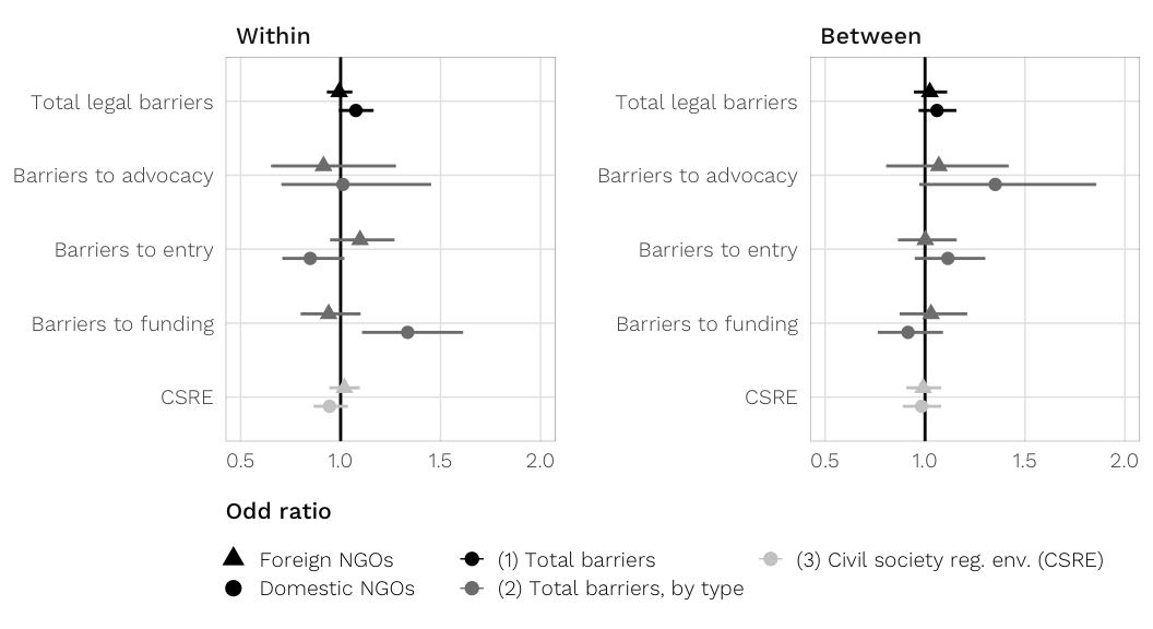
                                 vars.to.plot, exponentiate = TRUE)$melded.summary

coefs.raw.h3.dom <- mods.h3.dom.melded %>%
  left_join(coef.names.all, by = "term") %>%
  left_join(model.names, by = c("model.name" = "model")) %>%
  mutate(term = factor(term, levels = vars.to.plot, ordered = TRUE)) %>%
  arrange(desc(term)) %>%
  mutate(term_plot = ordered(fct_inorder(term_plot_short))) %>%
  mutate(coef.type = case_when(
    str_detect(.$term, "_within") ~ "Within",
    str_detect(.$term, "_between") ~ "Between",
  )) %>%
  mutate(coef.type = factor(coef.type, levels = c("Within", "Between"),
                            ordered = TRUE)) %>%
  mutate(model_clean = factor(model_clean, levels = rev(unique(model_clean)), ordered = TRUE))

mods.h3.foreign.melded <- bayes.meld(mods.h3.foreign.next_year.bayes,
                                     vars.to.plot, exponentiate = TRUE)$melded.summary

coefs.raw.h3.foreign <- mods.h3.foreign.melded %>%
  left_join(coef.names.all, by = "term") %>%
  left_join(model.names, by = c("model.name" = "model")) %>%
  mutate(term = factor(term, levels = vars.to.plot, ordered = TRUE)) %>%
  arrange(desc(term)) %>%
  mutate(term_plot = ordered(fct_inorder(term_plot_short))) %>%
  mutate(coef.type = case_when(
    str_detect(.$term, "_within") ~ "Within",
    str_detect(.$term, "_between") ~ "Between",
  )) %>%
  mutate(coef.type = factor(coef.type, levels = c("Within", "Between"),
                            ordered = TRUE)) %>%
  mutate(model_clean = factor(model_clean, levels = rev(unique(model_clean)), ordered = TRUE))

coefs.h3.both <- bind_rows(`Domestic NGOs` = coefs.raw.h3.dom,
                           `Foreign NGOs` = coefs.raw.h3.foreign,
                           .id = "channel")

fig.coefs.h3 <- ggplot(coefs.h3.both, aes(y = term_plot, x = med,
                                          colour = model_clean)) +
  geom_vline(xintercept = 1, colour = "black", size = 0.5) +
  geom_pointrangeh(aes(xmin = `2.5%`, xmax = `97.5%`, shape = channel),
                   size = 0.5, fatten = 3,
                   position = position_dodgev(height = 0.5)) +
  labs(x = "Percent change in ratio of aid channeled to NGO type (odds ratio)", y = NULL) +
  scale_colour_manual(values = model.colors) +
  expand_limits(x = c(0.5, 2)) +
  guides(color = guide_legend(override.aes = list(size = 0.25),
                              title = NULL, nrow = 2, order = 2),
         shape = guide_legend(override.aes = list(size = 0.5, linetype = 0),
                              title = NULL, nrow = 2, reverse = TRUE, order = 1)) +
  theme_donors() +
  theme(legend.justification = "left",
        legend.box.margin = margin(l = -0.75, t = -0.5, unit = "lines"),
        axis.title.x = element_text(hjust = 0)) +
  facet_wrap(~ coef.type, scales = "free", ncol = 2)
fig.coefs.h3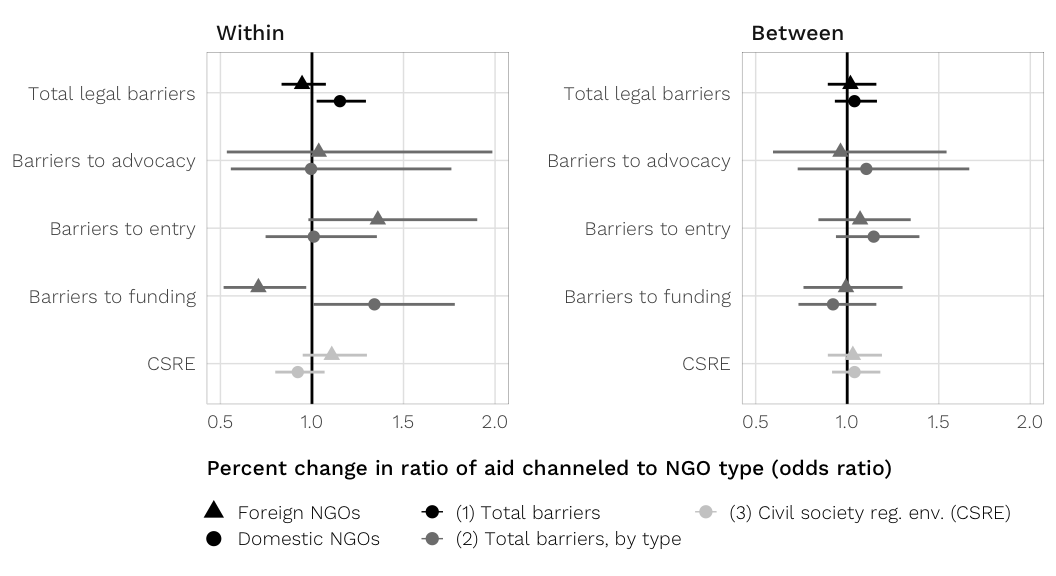
Proportion to domestic NGOs (nonimputed)
scales.h3.dom.next_year.no.imp <- mods.h3.dom.next_year.raw %>%
  filter(m == "original") %>%
  select(m, starts_with("scales")) %>%
  pull(scales_h3_dom.1) %>% .[[1]]

# Get model details and parameters
mods.h3.dom.next_year.bayes.no.imp <- mods.h3.dom.next_year.raw %>%
  select(-contains("scales")) %>%
  filter(m == "original") %>%
  gather(model.name, model, -m) %>%
  mutate(glance = model %>% map(glance),
         tidy = model %>% map(tidy, effects = "fixed")) %>%
  mutate(model_scale = model %>% map(add_scalemcmc))

h3_dom_coefs <- mods.h3.dom.next_year.bayes.no.imp %>%
  unnest(tidy) %>%
  filter(!duplicated(term, fromLast = TRUE)) %>%
  mutate(term_join = str_replace(term, "TRUE", "")) %>%
  left_join(coef.names.all, by = c("term_join" = "term")) %>%
  filter(term != "Intercept")

h3_dom_coefs_named <- h3_dom_coefs %>% pull(term) %>%
  set_names(h3_dom_coefs$term_clean)

huxreg(mods.h3.dom.next_year.bayes.no.imp$model_scale,
       coefs = c(h3_dom_coefs_named, Constant = "Intercept"),
       stars = NULL, statistics = c(N = "nobs"),
       tidy_args = list(conf.int = TRUE, prob = 0.95, exponentiate = TRUE,
                        effects = "fixed", scalings = scales.h3.dom.next_year.no.imp),
error_format = "({conf.low}, {conf.high})")| (1) | (2) | (3) | |
| Total legal barriers~within~ | 1.151 | ||
| (1.028, 1.295) | |||
| Total legal barriers~between~ | 1.034 | ||
| (0.924, 1.154) | |||
| Barriers to advocacy~within~ | 1.140 | ||
| (0.623, 2.114) | |||
| Barriers to advocacy~between~ | 1.136 | ||
| (0.762, 1.708) | |||
| Barriers to entry~within~ | 1.001 | ||
| (0.757, 1.335) | |||
| Barriers to entry~between~ | 1.133 | ||
| (0.928, 1.382) | |||
| Barriers to funding~within~ | 1.278 | ||
| (0.968, 1.706) | |||
| Barriers to funding~between~ | 0.906 | ||
| (0.729, 1.131) | |||
| Civil society reg. env. (CSRE)~within~ | 0.913 | ||
| (0.786, 1.057) | |||
| Civil society reg. env. (CSRE)~between~ | 1.025 | ||
| (0.908, 1.162) | |||
| Polity IV (0–10)~within~ | 0.878 | 0.881 | 0.908 |
| (0.789, 0.976) | (0.791, 0.987) | (0.799, 1.024) | |
| Polity IV (0–10)~between~ | 1.012 | 1.008 | 0.980 |
| (0.945, 1.086) | (0.936, 1.080) | (0.882, 1.089) | |
| GDP per capita (log)~within~ | 1.847 | 1.889 | 1.942 |
| (1.024, 3.239) | (1.057, 3.330) | (1.047, 3.544) | |
| GDP per capita (log)~between~ | 1.033 | 1.034 | 1.036 |
| (0.898, 1.183) | (0.903, 1.185) | (0.902, 1.185) | |
| Trade as % of GDP~within~ | 0.999 | 0.999 | 0.998 |
| (0.993, 1.005) | (0.993, 1.005) | (0.993, 1.004) | |
| Trade as % of GDP~between~ | 0.995 | 0.995 | 0.995 |
| (0.991, 0.999) | (0.991, 0.999) | (0.992, 0.999) | |
| Corruption~within~ | 1.208 | 1.214 | 1.186 |
| (1.036, 1.396) | (1.045, 1.411) | (1.015, 1.392) | |
| Corruption~between~ | 1.140 | 1.134 | 1.136 |
| (1.058, 1.231) | (1.048, 1.227) | (1.052, 1.227) | |
| Proportion of aid to domestic NGOs in present year (logit) | 1.411 | 1.406 | 1.415 |
| (1.337, 1.488) | (1.330, 1.484) | (1.344, 1.491) | |
| Internal conflict in last 5 years | 1.225 | 1.248 | 1.210 |
| (0.942, 1.585) | (0.959, 1.625) | (0.932, 1.543) | |
| Natural disasters | 0.990 | 0.988 | 0.992 |
| (0.961, 1.020) | (0.960, 1.017) | (0.963, 1.022) | |
| Constant | 0.022 | 0.021 | 0.028 |
| (0.005, 0.107) | (0.004, 0.109) | (0.007, 0.125) | |
| N | 1700 | 1700 | 1700 |
| . | |||
Proportion to foreign NGOs (nonimputed)
scales.h3.foreign.next_year.no.imp <- mods.h3.foreign.next_year.raw %>%
  filter(m == "original") %>%
  select(m, starts_with("scales")) %>%
  pull(scales_h3_foreign.1) %>% .[[1]]

# Get model details and parameters
mods.h3.foreign.next_year.bayes.no.imp <- mods.h3.foreign.next_year.raw %>%
  select(-contains("scales")) %>%
  filter(m == "original") %>%
  gather(model.name, model, -m) %>%
  mutate(glance = model %>% map(glance),
         tidy = model %>% map(tidy, effects = "fixed")) %>%
  mutate(model_scale = model %>% map(add_scalemcmc))

h3_foreign_coefs <- mods.h3.foreign.next_year.bayes.no.imp %>%
  unnest(tidy) %>%
  filter(!duplicated(term, fromLast = TRUE)) %>%
  mutate(term_join = str_replace(term, "TRUE", "")) %>%
  left_join(coef.names.all, by = c("term_join" = "term")) %>%
  filter(term != "Intercept")

h3_foreign_coefs_named <- h3_foreign_coefs %>% pull(term) %>%
  set_names(h3_foreign_coefs$term_clean)

huxreg(mods.h3.foreign.next_year.bayes.no.imp$model_scale,
       coefs = c(h3_foreign_coefs_named, Constant = "Intercept"),
       stars = NULL, statistics = c(N = "nobs"),
       tidy_args = list(conf.int = TRUE, prob = 0.95, exponentiate = TRUE,
                        effects = "fixed", scalings = scales.h3.foreign.next_year.no.imp),
error_format = "({conf.low}, {conf.high})")| (1) | (2) | (3) | |
| Total legal barriers~within~ | 0.950 | ||
| (0.836, 1.077) | |||
| Total legal barriers~between~ | 1.029 | ||
| (0.907, 1.168) | |||
| Barriers to advocacy~within~ | 1.068 | ||
| (0.550, 2.044) | |||
| Barriers to advocacy~between~ | 0.980 | ||
| (0.592, 1.609) | |||
| Barriers to entry~within~ | 1.360 | ||
| (0.991, 1.839) | |||
| Barriers to entry~between~ | 1.075 | ||
| (0.857, 1.373) | |||
| Barriers to funding~within~ | 0.705 | ||
| (0.524, 0.954) | |||
| Barriers to funding~between~ | 0.997 | ||
| (0.766, 1.300) | |||
| Civil society reg. env. (CSRE)~within~ | 1.146 | ||
| (0.974, 1.355) | |||
| Civil society reg. env. (CSRE)~between~ | 1.034 | ||
| (0.901, 1.194) | |||
| Polity IV (0–10)~within~ | 1.054 | 1.054 | 1.002 |
| (0.934, 1.187) | (0.938, 1.189) | (0.873, 1.153) | |
| Polity IV (0–10)~between~ | 0.991 | 0.985 | 0.957 |
| (0.915, 1.066) | (0.907, 1.068) | (0.843, 1.079) | |
| GDP per capita (log)~within~ | 0.262 | 0.253 | 0.251 |
| (0.154, 0.433) | (0.147, 0.435) | (0.148, 0.415) | |
| GDP per capita (log)~between~ | 0.724 | 0.721 | 0.725 |
| (0.626, 0.843) | (0.618, 0.845) | (0.623, 0.847) | |
| Trade as % of GDP~within~ | 0.996 | 0.996 | 0.997 |
| (0.990, 1.002) | (0.991, 1.002) | (0.991, 1.003) | |
| Trade as % of GDP~between~ | 0.999 | 0.999 | 0.999 |
| (0.995, 1.004) | (0.995, 1.004) | (0.995, 1.004) | |
| Corruption~within~ | 1.105 | 1.095 | 1.147 |
| (0.939, 1.307) | (0.926, 1.293) | (0.966, 1.364) | |
| Corruption~between~ | 1.293 | 1.288 | 1.288 |
| (1.183, 1.415) | (1.177, 1.408) | (1.180, 1.410) | |
| Proportion of aid to foreign NGOs in present year (logit) | 1.414 | 1.406 | 1.414 |
| (1.355, 1.480) | (1.346, 1.472) | (1.353, 1.481) | |
| Internal conflict in last 5 years | 1.180 | 1.196 | 1.217 |
| (0.882, 1.589) | (0.899, 1.613) | (0.906, 1.625) | |
| Natural disasters | 1.030 | 1.030 | 1.030 |
| (0.997, 1.064) | (0.997, 1.065) | (0.997, 1.065) | |
| Constant | 0.524 | 0.543 | 0.640 |
| (0.088, 3.142) | (0.091, 3.286) | (0.124, 3.333) | |
| N | 1700 | 1700 | 1700 |
| . | |||
Predicted proportion of aid channeled to domestic or foreign NGOs
model <- mods.h3.foreign.next_year.bayes %>%
  filter(m == "imp1", model.name == "mod.h3.foreign.barriers.total") %>%
  select(model) %>% .[[1]] %>% .[[1]]

new.data <- get_all_vars(model$formula, data = model$data) %>%
  select(-c(barriers.total_within, year, cowcode)) %>%
  summarise_all(typical) %>%
  mutate(id = 1) %>%
  right_join(expand.grid(barriers.total_within = seq(-3, 4, 0.5),
                         cowcode = 1000:1049,
                         year = 2000:2012,
                         id = 1), by = "id") %>% select(-id)

predicted.h3.foreign.barriers.total <- new.data %>%
  nest(-cowcode) %>%
  mutate(predicted = future_map(.x = data, ~ generate_predictions(.x))) %>%
  unnest() %>%
  mutate(ngo_type = "Foreign NGOs")

model <- mods.h3.dom.next_year.bayes %>%
  filter(m == "imp1", model.name == "mod.h3.barriers.total") %>%
  select(model) %>% .[[1]] %>% .[[1]]

new.data <- get_all_vars(model$formula, data = model$data) %>%
  select(-c(barriers.total_within, year, cowcode)) %>%
  summarise_all(typical) %>%
  mutate(id = 1) %>%
  right_join(expand.grid(barriers.total_within = seq(-3, 4, 0.5),
                         cowcode = 1000:1049,
                         year = 2000:2012,
                         id = 1), by = "id") %>% select(-id)

predicted.h3.dom.barriers.total <- new.data %>%
  nest(-cowcode) %>%
  mutate(predicted = future_map(.x = data, ~ generate_predictions(.x))) %>%
  unnest() %>%
  mutate(ngo_type = "Domestic NGOs")

df.plot.data.h3 <- bind_rows(predicted.h3.foreign.barriers.total,
                             predicted.h3.dom.barriers.total) %>%
  group_by(cowcode, ngo_type, barriers.total_within) %>%
  summarise_at(vars(predicted), funs(mean(.))) %>%
  ungroup() %>%
  mutate(value.fixed = inv.logit(predicted, a = 0.001))

df.plot.data.mean.h3 <- df.plot.data.h3 %>%
  group_by(ngo_type, barriers.total_within) %>%
  summarise(predicted = mean(predicted)) %>%
  mutate(value.fixed = inv.logit(predicted, a = 0.001)) %>%
  mutate(cowcode = 1)  # Fake country so the line plots
barriers.indiv.clean.names <- tribble(
~barrier, ~barrier.clean,
"advocacy_within", "Barriers to advocacy",
"entry_within", "Barriers to entry",
"funding_within", "Barriers to funding"
)
model <- mods.h3.foreign.next_year.bayes %>%
filter(m == "imp1", model.name == "mod.h3.foreign.type.total") %>%
select(model) %>% .[[1]] %>% .[[1]]
hypothetical.bounds <- get_all_vars(model$formula, data = model$data) %>%
select(advocacy_within, entry_within, funding_within) %>%
summarise_all(funs(min, max)) %>%
gather(key, value) %>%
mutate(value = round(value, 0)) %>%
# Have to separate on _m because of multiple _s, then re-add the m
separate(key, into = c("term", "variable"), sep = "_m") %>%
mutate(variable = paste0("m", variable)) %>%
spread(variable, value)
new.data.hypothetical.nested <- hypothetical.bounds %>%
nest(-term) %>%
mutate(newdata = map2(.x = data, .y = term,
~ expand.grid(term = seq(.x$min, .x$max, by = 0.5),
cowcode = 1000:1049,
year = 2000:2012,
id = 1) %>%
# Rename the term column to the actual term name
magrittr::set_colnames(c(.y, colnames(.)[-1]))))
new.data.hypothetical <- as_tibble(bind_rows(new.data.hypothetical.nested$newdata)) %>%
mutate_at(vars(contains("within")), funs(ifelse(is.na(.), 0, .)))
# Foreign NGOs
new.data <- get_all_vars(model$formula, data = model$data) %>%
select(-c(advocacy_within, entry_within, funding_within, year, cowcode)) %>%
summarise_all(typical) %>%
mutate(id = 1) %>%
right_join(new.data.hypothetical, by = "id") %>% select(-id)
predicted.h3.foreign.barriers.individual <- new.data %>%
nest(-cowcode) %>%
mutate(predicted = future_map(.x = data, ~ generate_predictions(.x))) %>%
unnest() %>%
mutate(ngo_type = "Foreign NGOs")
# Domestic NGOs
model <- mods.h3.dom.next_year.bayes %>%
filter(m == "imp1", model.name == "mod.h3.type.total") %>%
select(model) %>% .[[1]] %>% .[[1]]
new.data <- get_all_vars(model$formula, data = model$data) %>%
select(-c(advocacy_within, entry_within, funding_within, year, cowcode)) %>%
summarise_all(typical) %>%
mutate(id = 1) %>%
right_join(new.data.hypothetical, by = "id") %>% select(-id)
predicted.h3.dom.barriers.individual <- new.data %>%
nest(-cowcode) %>%
mutate(predicted = future_map(.x = data, ~ generate_predictions(.x))) %>%
unnest() %>%
mutate(ngo_type = "Domestic NGOs")
df.plot.data.indiv.h3 <- bind_rows(predicted.h3.foreign.barriers.individual,
predicted.h3.dom.barriers.individual) %>%
gather(barrier, barrier.value, c(advocacy_within, entry_within, funding_within)) %>%
group_by(cowcode, ngo_type, barrier.value, barrier) %>%
summarise_at(vars(predicted), funs(mean(.))) %>%
mutate(value.fixed = inv.logit(predicted, a = 0.001)) %>%
left_join(barriers.indiv.clean.names, by = "barrier")
df.plot.data.mean.indiv.h3 <- df.plot.data.indiv.h3 %>%
group_by(ngo_type, barrier, barrier.value) %>%
summarise(predicted = mean(predicted)) %>%
mutate(cowcode = 1) %>% # Fake country so the line plots
mutate(value.fixed = inv.logit(predicted, a = 0.001)) %>%
left_join(barriers.indiv.clean.names, by = "barrier")# Combine the two plot data frames
df.plot.data.both.h3 <- df.plot.data.h3 %>%
mutate(barrier = "barriers.total_within", barrier.clean = "Total barriers") %>%
rename(barrier.value = barriers.total_within) %>%
bind_rows(df.plot.data.indiv.h3) %>%
mutate(barrier.clean = ordered(fct_inorder(barrier.clean)),
highlight = ifelse(barrier.clean == "Total barriers", TRUE, FALSE)) %>%
mutate(ngo_type = recode(ngo_type,
`Domestic NGOs` = "Proportion channeled to domestic NGOs",
`Foreign NGOs` = "… to foreign NGOs"),
ngo_type = fct_inorder(ngo_type, ordered = TRUE))
df.plot.data.mean.both.h3 <- df.plot.data.mean.h3 %>%
mutate(barrier = "barriers.total_within", barrier.clean = "Total barriers") %>%
rename(barrier.value = barriers.total_within) %>%
bind_rows(df.plot.data.mean.indiv.h3) %>%
mutate(barrier.clean = ordered(fct_inorder(barrier.clean))) %>%
ungroup() %>%
mutate(ngo_type = recode(ngo_type,
`Domestic NGOs` = "Proportion channeled to domestic NGOs",
`Foreign NGOs` = "… to foreign NGOs"),
ngo_type = fct_inorder(ngo_type, ordered = TRUE))
# Create data frame for highlighting the total panel
df.panel.highlight.h3 <- df.plot.data.both.h3 %>%
distinct(barrier.clean, highlight)
fig.predicted.h3.barriers.both <-
ggplot(df.plot.data.both.h3,
aes(x = barrier.value, y = value.fixed, color = ngo_type,
group = interaction(ngo_type, cowcode))) +
geom_rect(data = df.panel.highlight.h3, aes(fill = highlight), inherit.aes = FALSE,
xmin = -Inf, xmax = Inf, ymin = -Inf, ymax = Inf, alpha = 0.15) +
geom_vline(xintercept = 0, colour = "black", size = 0.5) +
geom_smooth(method = "lm", size = 0.1, alpha = 0.1) +
geom_smooth(data = df.plot.data.mean.both.h3, size = 1, method = "lm") +
labs(x = "Difference from average level of NGO legislation in country (within effect)",
y = "Predicted proportion of\naid channeled to type of NGO\nin the following year") +
scale_y_continuous(labels = percent_format(accuracy = 1)) +
scale_fill_manual(values = c(NA, "grey50"), guide = FALSE) +
scale_color_manual(values = c("grey60", "black"), name = NULL) +
facet_wrap(~ barrier.clean, scales = "free_x", ncol = 2) +
theme_donors() +
theme(axis.title.x = element_text(hjust = 0),
legend.justification = "left",
legend.margin = margin(l = 0))
fig.predicted.h3.barriers.both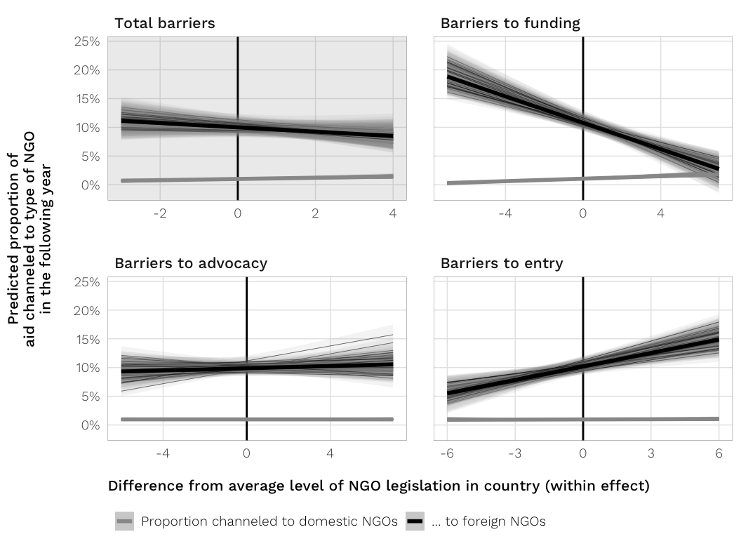
Save data
Save CSVs of predicted data for use in other projects
predictions <- tribble(
  ~prediction,                              ~filename,
  predicted.h1.barriers.total,              "predicted_h1_barriers_total",
  predicted.h1.barriers.individual,         "predicted_h1_barriers_individual",
  predicted.h2.barriers.total,              "predicted_h2_barriers_total",
  predicted.h2.barriers.individual,         "predicted_h2_barriers_individual",
  predicted.h3.dom.barriers.total,          "predicted_h3_dom_barriers_total",
  predicted.h3.dom.barriers.individual,     "predicted_h3_dom_barriers_individual",
  predicted.h3.foreign.barriers.total,      "predicted_h3_foreign_barriers_total",
  predicted.h3.foreign.barriers.individual, "predicted_h3_foreign_barriers_individual"
) %>%
  walk2(.x = .$prediction, .y = .$filename,
        .f = ~ write_csv(.x, path = here("Data", "data_export", paste0(.y, ".csv"))))
H2: Zero-one-inflated beta
The big caveat here is that we can’t do a 1:1 mapping of these coefficients to the fractional logit models, since the coefficients here only apply to the non-zero and non-one parts of the model. What’s important for robustness is that the coefficients all go in the same direction as the fractional logit model (though with less significance, since different parts of the model explain the presence/absence significance).
# Get scaling factors
scales.h2.next_year.zoib <- mods.h2.next_year.raw.bayes.zoib %>%
  filter(m != "original") %>%
  select(m, starts_with("scales")) %>%
  gather(scales.name, scales, -m)

# Get model details and parameters
mods.h2.next_year.bayes.zoib <- mods.h2.next_year.raw.bayes.zoib %>%
  filter(m != "original") %>%
  select(m, starts_with("mod")) %>%
  gather(model.name, model, -m) %>%
  mutate(glance = model %>% map(glance),
         tidy = model %>% map(tidy)) %>%
  bind_cols(select(scales.h2.next_year.zoib, -m))
MCMC diagnostics
Check fit
Again, use one of the imputed models (mod.h2.barriers.total.zoib) to check for fit and convergence.
model.to.check <- mods.h2.next_year.bayes.zoib %>%
  filter(m == "imp1", model.name == "mod.h2.barriers.total.zoib") %>%
  select(model) %>% .[[1]] %>% .[[1]]
Posterior predictive distribution vs. observed outcome?
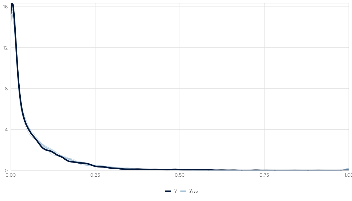
Check convergence
Chain convergence:
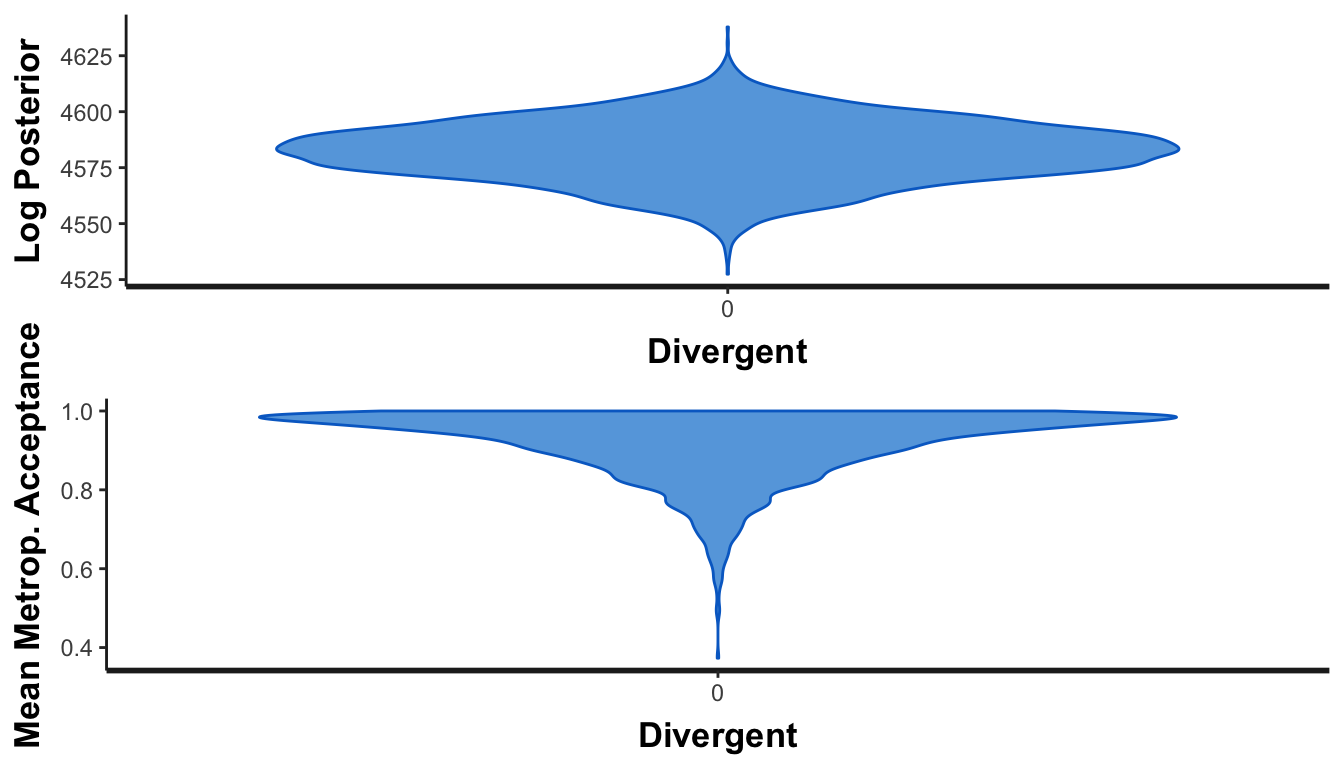
Results
Coefficients
vars.to.plot <- c("barriers.total_within", "barriers.total_between",
                  "advocacy_within", "advocacy_between",
                  "entry_within", "entry_between",
                  "funding_within", "funding_between",
                  "csre_within", "csre_between")

mods.h2.melded.zoib <- bayes.meld(mods.h2.next_year.bayes.zoib,
                                  vars.to.plot, exponentiate = TRUE)$melded.summary

plot.data <- mods.h2.melded.zoib %>%
  left_join(coef.names.all, by = "term") %>%
  left_join(model.names, by = c("model.name" = "model")) %>%
  mutate(term = factor(term, levels = vars.to.plot, ordered = TRUE)) %>%
  arrange(desc(term)) %>%
  mutate(term_plot = ordered(fct_inorder(term_plot_short))) %>%
  mutate(coef.type = case_when(
    str_detect(.$term, "_within") ~ "Within",
    str_detect(.$term, "_between") ~ "Between",
  )) %>%
  mutate(coef.type = factor(coef.type, levels = c("Within", "Between"),
                            ordered = TRUE)) %>%
  mutate(model_clean = factor(model_clean, levels = rev(unique(model_clean)), ordered = TRUE))

fig.coefs.h2.zoib <- ggplot(plot.data, aes(x = med, y = term_plot, colour = model_clean)) +
  geom_vline(xintercept = 1, colour = "black", size = 0.5) +
  geom_pointrangeh(aes(xmin = `2.5%`, xmax = `97.5%`), size = 0.5, fatten = 3) +
  labs(x = "Odds ratio ", y = NULL) +
  scale_colour_manual(values = model.colors, name = NULL) +
  expand_limits(x = c(0.6, 1.3)) +
  guides(color = guide_legend(override.aes = list(size = 0.25))) +
  theme_donors() +
  theme(legend.justification = "left",
        legend.box.margin = margin(l = -0.75, t = -0.5, unit = "lines"),
        axis.title.x = element_text(hjust = 0)) +
  facet_wrap(~ coef.type, scales = "free", ncol = 2)
fig.coefs.h2.zoib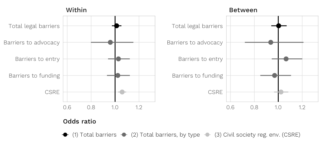
Complete results in a table
caption <- "The effect of anti-NGO legislation on the proportion of OECD overseas development assistance (ODA) committed to contentious purposes in the following year (H~2~), full models. Each cell contains the parameter's posterior median, the 95% credible interval, and the probability that the parameter is greater than one (in italics). {#tbl:h2-coefs-zoib}"
note <- c("Zero-one-inflated beta models. Odds ratios reported.")

table.h2.zoib <- bayesgazer(mods.h2.next_year.bayes.zoib, exponentiate = TRUE,
                            caption = caption, note = note)

cat(table.h2.zoib)| (1) | (2) | (3) | |
|---|---|---|---|
| Fixed part (odds ratios) | |||
| Total legal barrierswithin | 1.01 (0.97, 1.05); 0.74 |
||
| Total legal barriersbetween | 1.00 (0.94, 1.07); 0.54 |
||
| Barriers to advocacywithin | 0.96 (0.80, 1.15); 0.33 |
||
| Barriers to advocacybetween | 0.94 (0.72, 1.21); 0.32 |
||
| Barriers to entrywithin | 1.03 (0.94, 1.12); 0.73 |
||
| Barriers to entrybetween | 1.07 (0.95, 1.20); 0.85 |
||
| Barriers to fundingwithin | 1.02 (0.93, 1.12); 0.68 |
||
| Barriers to fundingbetween | 0.97 (0.85, 1.11); 0.32 |
||
| 0.18 (0.17, 0.20); 0.00 |
0.18 (0.17, 0.20); 0.00 |
0.18 (0.17, 0.20); 0.00 |
|
| 0.03 (0.02, 0.04); 0.00 |
0.03 (0.02, 0.04); 0.00 |
0.03 (0.02, 0.04); 0.00 |
|
| Civil society reg. env. (CSRE)within | 1.06 (1.02, 1.09); 1.00 |
||
| Civil society reg. env. (CSRE)between | 1.02 (0.97, 1.08); 0.78 |
||
| Polity IV (0–10)within | 1.03 (1.00, 1.05); 0.99 |
1.03 (1.00, 1.05); 0.98 |
0.99 (0.96, 1.02); 0.34 |
| Polity IV (0–10)between | 1.04 (1.01, 1.08); 0.99 |
1.04 (1.00, 1.07); 0.98 |
1.02 (0.97, 1.08); 0.79 |
| GDP per capita (log)within | 0.90 (0.78, 1.02); 0.05 |
0.89 (0.78, 1.02); 0.05 |
0.90 (0.78, 1.03); 0.06 |
| GDP per capita (log)between | 0.84 (0.78, 0.89); 0.00 |
0.84 (0.78, 0.90); 0.00 |
0.84 (0.79, 0.89); 0.00 |
| Trade as % of GDPwithin | 1.00 (1.00, 1.00); 0.11 |
1.00 (1.00, 1.00); 0.11 |
1.00 (1.00, 1.00); 0.10 |
| Trade as % of GDPbetween | 1.00 (1.00, 1.00); 0.99 |
1.00 (1.00, 1.00); 0.99 |
1.00 (1.00, 1.00); 0.99 |
| Corruptionwithin | 1.00 (0.97, 1.04); 0.57 |
1.00 (0.97, 1.04); 0.56 |
1.01 (0.97, 1.05); 0.69 |
| Corruptionbetween | 1.04 (1.00, 1.08); 0.97 |
1.04 (1.00, 1.07); 0.96 |
1.04 (1.00, 1.08); 0.98 |
| Proportion of contentious aid | 4.83 (3.61, 6.43); 1.00 |
4.78 (3.55, 6.38); 1.00 |
4.80 (3.56, 6.40); 1.00 |
| Internal conflict in last 5 years | 1.01 (0.93, 1.10); 0.61 |
1.01 (0.93, 1.10); 0.59 |
1.03 (0.94, 1.12); 0.71 |
| Natural disasters | 0.99 (0.98, 1.01); 0.19 |
0.99 (0.98, 1.01); 0.20 |
0.99 (0.98, 1.01); 0.12 |
| After 1989 | 2.35 (1.75, 3.18); 1.00 |
2.36 (1.75, 3.18); 1.00 |
2.21 (1.64, 2.94); 1.00 |
| Constant | 0.06 (0.03, 0.13); 0.00 |
0.06 (0.03, 0.12); 0.00 |
0.07 (0.03, 0.13); 0.00 |
| Random part (original coefficients) | |||
| Within-country variability | 0.35 | 0.36 | 0.35 |
| Within-year variability | 0.35 | 0.36 | 0.35 |
| Model details | |||
| Imputed datasets (m) | 5 | 5 | 5 |
| N | 3922 | 3922 | 3922 |
| Posterior sample size | 4000 | 4000 | 4000 |
| Notes | |||
| Zero-one-inflated beta models. Odds ratios reported. |
H3: Zero-one-inflated beta
# Get scaling factors
scales.h3.dom.next_year.zoib <- mods.h3.dom.next_year.raw.zoib %>%
  filter(m != "original") %>%
  select(m, starts_with("scales")) %>%
  gather(scales.name, scales, -m)

# Get model details and parameters
mods.h3.dom.next_year.bayes.zoib <- mods.h3.dom.next_year.raw.zoib %>%
  filter(m != "original") %>%
  select(m, starts_with("mod")) %>%
  gather(model.name, model, -m) %>%
  mutate(glance = model %>% map(glance),
         tidy = model %>% map(tidy)) %>%
  bind_cols(select(scales.h3.dom.next_year.zoib, -m))
# Get scaling factors
scales.h3.foreign.next_year.zoib <- mods.h3.foreign.next_year.raw.zoib %>%
filter(m != "original") %>%
select(m, starts_with("scales")) %>%
gather(scales.name, scales, -m)
# Get model details and parameters
mods.h3.foreign.next_year.bayes.zoib <- mods.h3.foreign.next_year.raw.zoib %>%
filter(m != "original") %>%
select(m, starts_with("mod")) %>%
gather(model.name, model, -m) %>%
mutate(glance = model %>% map(glance),
tidy = model %>% map(tidy)) %>%
bind_cols(select(scales.h3.foreign.next_year.zoib, -m))MCMC diagnostics
Check fit
Again, use one of the imputed models (mod.h3.barriers.total.zoib) to check for fit and convergence.
model.to.check <- mods.h3.dom.next_year.bayes.zoib %>%
  filter(m == "imp1", model.name == "mod.h3.barriers.total") %>%
  select(model) %>% .[[1]] %>% .[[1]]
Posterior predictive distribution vs. observed outcome?
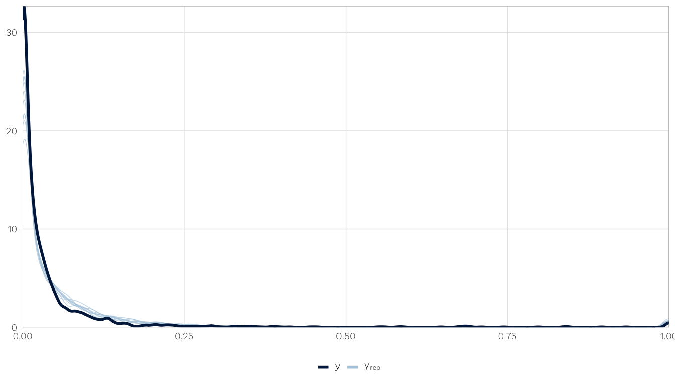
Check convergence
Chain convergence:
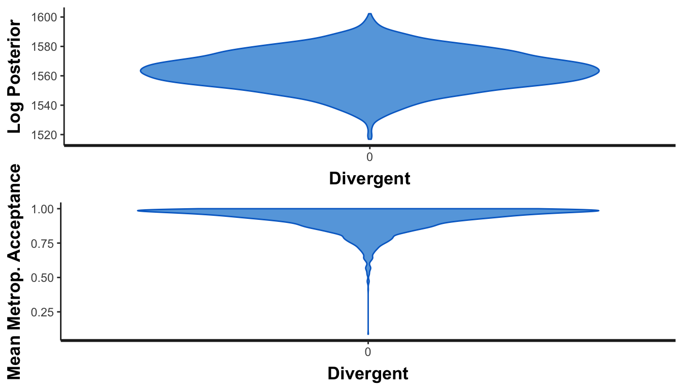
Results
Proportion to domestic NGOs
caption <- "The effect of anti-NGO legislation on the proportion of US aid channeled through *domestic* NGOs in the following year (H~3~), full models. Each cell contains the parameter's posterior median, the 95% credible interval, and the probability that the parameter is greater than one (in italics) {#tbl:h3-domestic-coefs-zoib}"
note <- c("Zero-one-inflated beta models. Odds ratios reported.")

table.h3.domestic.zoib <- bayesgazer(mods.h3.dom.next_year.bayes.zoib,
                                     caption = caption, note = note, exponentiate = TRUE)

cat(table.h3.domestic.zoib)| (1) | (2) | (3) | |
|---|---|---|---|
| Fixed part (odds ratios) | |||
| Total legal barrierswithin | 1.08 (0.99, 1.17); 0.96 |
||
| Total legal barriersbetween | 1.06 (0.97, 1.16); 0.90 |
||
| Barriers to advocacywithin | 1.01 (0.70, 1.45); 0.53 |
||
| Barriers to advocacybetween | 1.35 (0.97, 1.86); 0.96 |
||
| Barriers to entrywithin | 0.85 (0.71, 1.02); 0.04 |
||
| Barriers to entrybetween | 1.11 (0.95, 1.30); 0.91 |
||
| Barriers to fundingwithin | 1.34 (1.11, 1.61); 1.00 |
||
| Barriers to fundingbetween | 0.91 (0.76, 1.09); 0.15 |
||
| 0.38 (0.35, 0.43); 0.00 |
0.39 (0.35, 0.43); 0.00 |
0.39 (0.35, 0.43); 0.00 |
|
| 0.05 (0.03, 0.07); 0.00 |
0.05 (0.03, 0.07); 0.00 |
0.05 (0.03, 0.07); 0.00 |
|
| Civil society reg. env. (CSRE)within | 0.94 (0.87, 1.04); 0.11 |
||
| Civil society reg. env. (CSRE)between | 0.98 (0.89, 1.08); 0.36 |
||
| Polity IV (0–10)within | 0.94 (0.88, 1.01); 0.05 |
0.94 (0.88, 1.02); 0.06 |
0.96 (0.88, 1.04); 0.15 |
| Polity IV (0–10)between | 1.01 (0.95, 1.07); 0.62 |
1.01 (0.95, 1.07); 0.58 |
1.00 (0.92, 1.09); 0.52 |
| GDP per capita (log)within | 1.57 (1.02, 2.28); 0.98 |
1.55 (1.01, 2.28); 0.98 |
1.72 (1.10, 2.50); 0.99 |
| GDP per capita (log)between | 1.17 (1.05, 1.29); 1.00 |
1.17 (1.05, 1.30); 1.00 |
1.17 (1.05, 1.30); 1.00 |
| Trade as % of GDPwithin | 1.00 (1.00, 1.01); 0.70 |
1.00 (1.00, 1.00); 0.69 |
1.00 (1.00, 1.01); 0.71 |
| Trade as % of GDPbetween | 1.00 (0.99, 1.00); 0.06 |
1.00 (0.99, 1.00); 0.03 |
1.00 (0.99, 1.00); 0.04 |
| Corruptionwithin | 1.05 (0.97, 1.14); 0.88 |
1.06 (0.98, 1.16); 0.92 |
1.03 (0.95, 1.12); 0.76 |
| Corruptionbetween | 1.02 (0.96, 1.09); 0.75 |
1.02 (0.95, 1.09); 0.69 |
1.02 (0.95, 1.08); 0.69 |
| Proportion of aid to domestic NGOs | 4.79 (3.34, 6.90); 1.00 |
4.51 (3.12, 6.47); 1.00 |
4.58 (3.15, 6.61); 1.00 |
| Internal conflict in last 5 years | 1.03 (0.87, 1.22); 0.63 |
1.03 (0.87, 1.23); 0.64 |
1.02 (0.86, 1.22); 0.60 |
| Natural disasters | 0.98 (0.96, 1.00); 0.05 |
0.98 (0.96, 1.00); 0.02 |
0.98 (0.96, 1.00); 0.06 |
| Constant | 0.01 (0.00, 0.04); 0.00 |
0.01 (0.00, 0.04); 0.00 |
0.01 (0.00, 0.05); 0.00 |
| Random part (original coefficients) | |||
| Within-country variability | 0.59 | 0.59 | 0.60 |
| Within-year variability | 0.10 | 0.10 | 0.10 |
| Model details | |||
| Imputed datasets (m) | 5 | 5 | 5 |
| N | 1751 | 1751 | 1751 |
| Posterior sample size | 4000 | 4000 | 4000 |
| Notes | |||
| Zero-one-inflated beta models. Odds ratios reported. |
Proportion to foreign NGOs
caption <- "The effect of anti-NGO legislation on the proportion of US aid channeled through *US-based and international* NGOs in the following year (H~3~), full models. Each cell contains the parameter's posterior median, the 95% credible interval, and the probability that the parameter is greater than one (in italics) {#tbl:h3-foreign-coefs-zoib}"
note <- c("Zero-one-inflated beta models. Odds ratios reported.")

table.h3.domestic.zoib <- bayesgazer(mods.h3.foreign.next_year.bayes.zoib,
                                     caption = caption, note = note, exponentiate = TRUE)

cat(table.h3.domestic.zoib)| (1) | (2) | (3) | |
|---|---|---|---|
| Fixed part (odds ratios) | |||
| Total legal barrierswithin | 0.99 (0.93, 1.06); 0.41 |
||
| Total legal barriersbetween | 1.02 (0.94, 1.11); 0.71 |
||
| Barriers to advocacywithin | 0.91 (0.65, 1.28); 0.31 |
||
| Barriers to advocacybetween | 1.07 (0.81, 1.42); 0.68 |
||
| Barriers to entrywithin | 1.10 (0.95, 1.27); 0.89 |
||
| Barriers to entrybetween | 1.00 (0.86, 1.16); 0.51 |
||
| Barriers to fundingwithin | 0.94 (0.80, 1.10); 0.22 |
||
| Barriers to fundingbetween | 1.03 (0.87, 1.21); 0.64 |
||
| 0.27 (0.24, 0.30); 0.00 |
0.27 (0.24, 0.30); 0.00 |
0.27 (0.24, 0.30); 0.00 |
|
| 0.06 (0.04, 0.09); 0.00 |
0.06 (0.04, 0.09); 0.00 |
0.06 (0.04, 0.09); 0.00 |
|
| Civil society reg. env. (CSRE)within | 1.02 (0.94, 1.10); 0.69 |
||
| Civil society reg. env. (CSRE)between | 0.99 (0.91, 1.08); 0.41 |
||
| Polity IV (0–10)within | 0.92 (0.87, 0.97); 0.00 |
0.91 (0.86, 0.97); 0.00 |
0.91 (0.86, 0.97); 0.00 |
| Polity IV (0–10)between | 0.94 (0.89, 0.99); 0.01 |
0.94 (0.89, 0.99); 0.01 |
0.94 (0.87, 1.02); 0.06 |
| GDP per capita (log)within | 0.56 (0.44, 0.73); 0.00 |
0.56 (0.44, 0.71); 0.00 |
0.56 (0.44, 0.71); 0.00 |
| GDP per capita (log)between | 0.91 (0.83, 1.01); 0.03 |
0.91 (0.83, 1.00); 0.03 |
0.91 (0.83, 1.00); 0.03 |
| Trade as % of GDPwithin | 1.00 (0.99, 1.00); 0.05 |
1.00 (0.99, 1.00); 0.05 |
1.00 (0.99, 1.00); 0.05 |
| Trade as % of GDPbetween | 1.00 (1.00, 1.00); 0.84 |
1.00 (1.00, 1.01); 0.83 |
1.00 (1.00, 1.00); 0.82 |
| Corruptionwithin | 1.06 (0.98, 1.15); 0.93 |
1.06 (0.98, 1.15); 0.91 |
1.07 (0.99, 1.16); 0.94 |
| Corruptionbetween | 1.06 (1.00, 1.12); 0.97 |
1.06 (1.00, 1.13); 0.97 |
1.05 (1.00, 1.12); 0.96 |
| Proportion of aid to foreign NGOs | 3.61 (2.78, 4.67); 1.00 |
3.57 (2.75, 4.64); 1.00 |
3.62 (2.80, 4.71); 1.00 |
| Internal conflict in last 5 years | 1.09 (0.95, 1.26); 0.88 |
1.09 (0.95, 1.26); 0.89 |
1.09 (0.95, 1.25); 0.87 |
| Natural disasters | 1.01 (0.99, 1.02); 0.79 |
1.01 (0.99, 1.02); 0.78 |
1.01 (0.99, 1.02); 0.80 |
| Constant | 0.37 (0.12, 1.08); 0.03 |
0.37 (0.12, 1.10); 0.04 |
0.41 (0.15, 1.10); 0.04 |
| Random part (original coefficients) | |||
| Within-country variability | 0.53 | 0.54 | 0.53 |
| Within-year variability | 0.04 | 0.04 | 0.04 |
| Model details | |||
| Imputed datasets (m) | 5 | 5 | 5 |
| N | 1751 | 1751 | 1751 |
| Posterior sample size | 4000 | 4000 | 4000 |
| Notes | |||
| Zero-one-inflated beta models. Odds ratios reported. |
Plot of proportion to domestic and foreign NGOs
vars.to.plot <- c("barriers.total_within", "barriers.total_between",
                  "advocacy_within", "advocacy_between",
                  "entry_within", "entry_between",
                  "funding_within", "funding_between",
                  "csre_within", "csre_between")

mods.h3.dom.melded.zoib <- bayes.meld(mods.h3.dom.next_year.bayes.zoib,
                                      vars.to.plot, exponentiate = TRUE)$melded.summary

coefs.raw.h3.dom.zoib <- mods.h3.dom.melded.zoib %>%
  left_join(coef.names.all, by = "term") %>%
  left_join(model.names, by = c("model.name" = "model")) %>%
  mutate(term = factor(term, levels = vars.to.plot, ordered = TRUE)) %>%
  arrange(desc(term)) %>%
  mutate(term_plot = ordered(fct_inorder(term_plot_short))) %>%
  mutate(coef.type = case_when(
    str_detect(.$term, "_within") ~ "Within",
    str_detect(.$term, "_between") ~ "Between",
  )) %>%
  mutate(coef.type = factor(coef.type, levels = c("Within", "Between"),
                            ordered = TRUE)) %>%
  mutate(model_clean = factor(model_clean, levels = rev(unique(model_clean)), ordered = TRUE))

mods.h3.foreign.melded.zoib <- bayes.meld(mods.h3.foreign.next_year.bayes.zoib,
                                          vars.to.plot, exponentiate = TRUE)$melded.summary

coefs.raw.h3.foreign.zoib <- mods.h3.foreign.melded.zoib %>%
  left_join(coef.names.all, by = "term") %>%
  left_join(model.names, by = c("model.name" = "model")) %>%
  mutate(term = factor(term, levels = vars.to.plot, ordered = TRUE)) %>%
  arrange(desc(term)) %>%
  mutate(term_plot = ordered(fct_inorder(term_plot_short))) %>%
  mutate(coef.type = case_when(
    str_detect(.$term, "_within") ~ "Within",
    str_detect(.$term, "_between") ~ "Between",
  )) %>%
  mutate(coef.type = factor(coef.type, levels = c("Within", "Between"),
                            ordered = TRUE)) %>%
  mutate(model_clean = factor(model_clean, levels = rev(unique(model_clean)), ordered = TRUE))

coefs.h3.both.zoib <- bind_rows(`Domestic NGOs` = coefs.raw.h3.dom.zoib,
                                `Foreign NGOs` = coefs.raw.h3.foreign.zoib,
                                .id = "channel")

fig.coefs.h3.zoib <- ggplot(coefs.h3.both.zoib, aes(y = term_plot, x = med,
                                                    colour = model_clean)) +
  geom_vline(xintercept = 1, colour = "black", size = 0.5) +
  geom_pointrangeh(aes(xmin = `2.5%`, xmax = `97.5%`, shape = channel),
                   size = 0.5, fatten = 3,
                   position = position_dodgev(height = 0.5)) +
  labs(x = "Odd ratio", y = NULL) +
  scale_colour_manual(values = model.colors) +
  expand_limits(x = c(0.5, 2)) +
  guides(color = guide_legend(override.aes = list(size = 0.25),
                              title = NULL, nrow = 2, order = 2),
         shape = guide_legend(override.aes = list(size = 0.5, linetype = 0),
                              title = NULL, nrow = 2, reverse = TRUE, order = 1)) +
  theme_donors() +
  theme(legend.justification = "left",
        legend.box.margin = margin(l = -0.75, t = -0.5, unit = "lines"),
        axis.title.x = element_text(hjust = 0)) +
  facet_wrap(~ coef.type, scales = "free", ncol = 2)
fig.coefs.h3.zoib