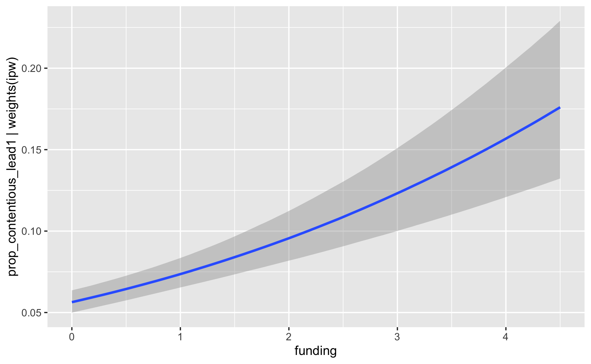
H₂: Effect of anti-NGO crackdown on aid contentiousness

library(tidyverse)
library(brms)
library(tidybayes)
library(bayesplot)
library(fixest)
library(broom)
library(broom.mixed)
library(modelsummary)
library(patchwork)
library(tictoc)
library(latex2exp)
library(scales)
library(extraDistr)
library(glue)
library(here)

source(here("lib", "graphics.R"))
source(here("lib", "misc_funs.R"))
color_scheme_set("viridisC")

labs_exp_logged <- function(brks) {TeX(paste0("e^{", as.character(log(brks))), "}")}
labs_exp <- function(brks) {TeX(paste0("e^{", as.character(brks)), "}")}

my_seed <- 1234
set.seed(my_seed)

options(mc.cores = parallel::detectCores(),  # Use all possible cores
        brms.backend = "rstan")

CHAINS <- 4
ITER <- 2000
WARMUP <- 1000
BAYES_SEED <- 1234

df_country_aid <- readRDS(here("data", "derived_data", "df_country_aid.rds"))

df_country_aid <- df_country_aid %>% 
  # Winsorize prop_contentious for the two cases that are exactly 1
  mutate(prop_contentious_orig = prop_contentious,
         prop_contentious = ifelse(prop_contentious == 1, 0.999, prop_contentious),
         prop_contentious_lead1_orig = prop_contentious_lead1,
         prop_contentious_lead1 = 
           ifelse(prop_contentious_lead1 == 1, 0.999, prop_contentious_lead1),
         prop_contentious_lead1 = 
           ifelse(prop_contentious_lead1 < 0, 0, prop_contentious_lead1))

df_country_aid_laws <- filter(df_country_aid, laws)

Weight models

• Numerator is lagged treatment + non-varying confounders
• Denominator is lagged treatment + lagged outcome + time-varying confounders + non-varying confounders

\[ sw = \prod^t_{t = 1} \frac{\phi(T_{it} | T_{i, t-1}, C_i)}{\phi(T_{it} | T_{i, t-1}, D_{i, t-1}, C_i)} \]

Priors for weight models

We use generic weakly informative priors for our model parameters:

• Intercept: \(\mathcal{N} (0, 10)\)
• Coefficients: \(\mathcal{N} (0, 2.5)\)
• Sigma: \(\operatorname{Cauchy} (0, 1)\)

pri_int <- ggplot() +
  stat_function(fun = dnorm, args = list(mean = 0, sd = 10),
                geom = "area", fill = "grey80", color = "black") +
  labs(x = TeX("\\textbf{Intercept (β_0)}")) +
  annotate(geom = "label", x = 0, y = 0.01, label = "N(0, 10)", size = pts(9)) +
  xlim(-40, 40) +
  theme_donors(prior = TRUE)

pri_coef <- ggplot() +
  stat_function(fun = dnorm, args = list(mean = 0, sd = 2.5),
                geom = "area", fill = "grey80", color = "black") +
  labs(x = TeX("\\textbf{Coefficients (β_x)}")) +
  annotate(geom = "label", x = 0, y = 0.04, label = "N(0, 3)", size = pts(9)) +
  xlim(-10, 10) +
  theme_donors(prior = TRUE)

pri_sigma <- ggplot() +
  stat_function(fun = dcauchy, args = list(location = 0, scale = 1),
                geom = "area", fill = "grey80", color = "black") +
  labs(x = "σ") +
  annotate(geom = "label", x = 5, y = 0.08, label = "Cauchy(0, 1)", size = pts(9)) +
  xlim(0, 10) +
  theme_donors(prior = TRUE)

(pri_int + pri_coef + pri_sigma)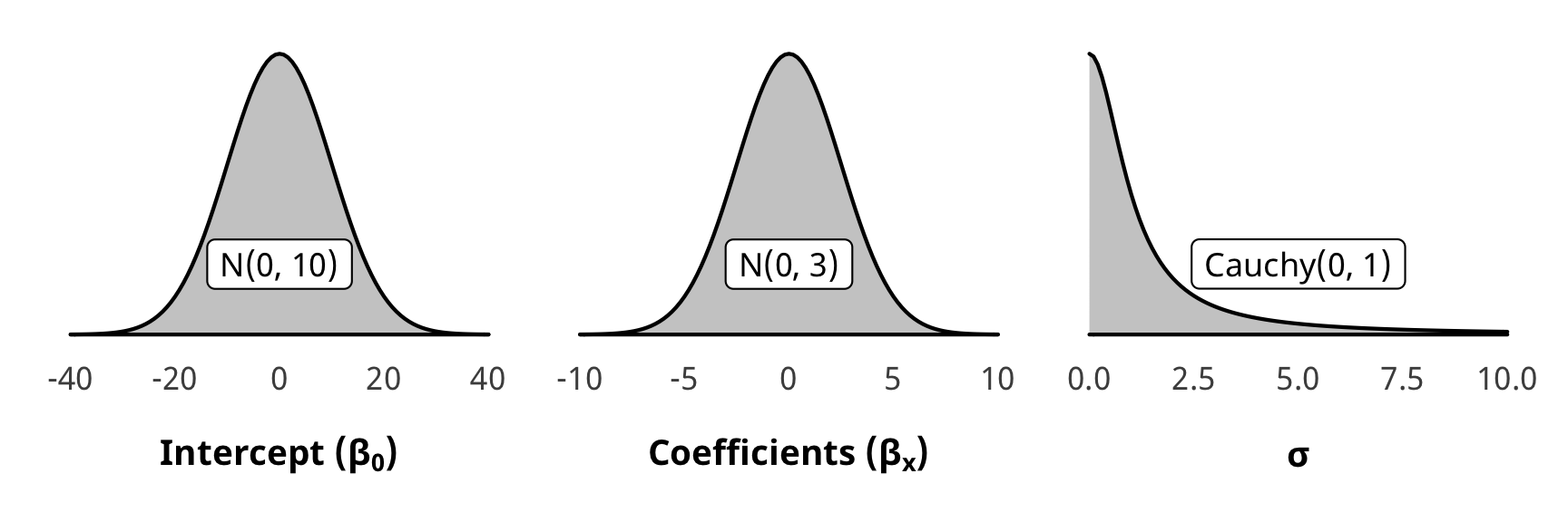

Run weight models

# Numerator ---------------------------------------------------------------
# Formulas
# Treatment ~ lag treatment + non-varying confounders
formula_h2_num_total <- bf(barriers_total ~ barriers_total_lag1 + (1 | gwcode))
formula_h2_num_advocacy <- bf(advocacy ~ advocacy_lag1 + (1 | gwcode))
formula_h2_num_entry <- bf(entry ~ entry_lag1 + (1 | gwcode))
formula_h2_num_funding <- bf(funding ~ funding_lag1 + (1 | gwcode))

# Priors
prior_num <- c(set_prior("normal(0, 10)", class = "Intercept"),
               set_prior("normal(0, 2.5)", class = "b"),
               set_prior("cauchy(0, 1)", class = "sd"))


# Denominator -------------------------------------------------------------
# Formulas
# Treatment ~ lag treatment + lag outcome + varying confounders + non-varying confounders
formula_h2_denom_total <- 
  bf(barriers_total ~ barriers_total_lag1 + prop_contentious_lag1 +
       # Human rights and politics
       v2x_polyarchy + v2x_corr + v2x_rule + v2x_civlib + v2x_clphy + v2x_clpriv +
       # Economics and development
       gdpcap_log + un_trade_pct_gdp + v2peedueq + v2pehealth + e_peinfmor +
       # Conflict and disasters
       internal_conflict_past_5 + natural_dis_count +
       (1 | gwcode))

formula_h2_denom_advocacy <- 
  bf(advocacy ~ advocacy_lag1 + prop_contentious_lag1 +
       v2x_polyarchy + v2x_corr + v2x_rule + v2x_civlib + v2x_clphy + v2x_clpriv +
       gdpcap_log + un_trade_pct_gdp + v2peedueq + v2pehealth + e_peinfmor +
       internal_conflict_past_5 + natural_dis_count +
       (1 | gwcode))

formula_h2_denom_entry <- 
  bf(entry ~ entry_lag1 + prop_contentious_lag1 +
       v2x_polyarchy + v2x_corr + v2x_rule + v2x_civlib + v2x_clphy + v2x_clpriv +
       gdpcap_log + un_trade_pct_gdp + v2peedueq + v2pehealth + e_peinfmor +
       internal_conflict_past_5 + natural_dis_count +
       (1 | gwcode))

formula_h2_denom_funding <- 
  bf(funding ~ funding_lag1 + prop_contentious_lag1 +
       v2x_polyarchy + v2x_corr + v2x_rule + v2x_civlib + v2x_clphy + v2x_clpriv +
       gdpcap_log + un_trade_pct_gdp + v2peedueq + v2pehealth + e_peinfmor +
       internal_conflict_past_5 + natural_dis_count +
       (1 | gwcode))

# Priors
prior_denom <- c(set_prior("normal(0, 10)", class = "Intercept"),
                 set_prior("normal(0, 2.5)", class = "b"),
                 set_prior("normal(0, 2.5)", class = "sd"))


# Run weighting models ----------------------------------------------------
# All models get run inside a tibble using map() magic
all_models_h2 <- tribble(
  ~model_name, ~formula_num, ~formula_denom,
  "h2_total", formula_h2_num_total, formula_h2_denom_total,
  "h2_advocacy", formula_h2_num_advocacy, formula_h2_denom_advocacy,
  "h2_entry", formula_h2_num_entry, formula_h2_denom_entry,
  "h2_funding", formula_h2_num_funding, formula_h2_denom_funding
)

# Fit models
tic()
fit_h2_all_models <- all_models_h2 %>%
  mutate(fit_num = map2(formula_num, model_name, ~brm(
    .x,
    data = df_country_aid_laws,
    prior = prior_num,
    iter = ITER, chains = CHAINS, warmup = WARMUP, seed = BAYES_SEED,
    control = list(adapt_delta = 0.99),
    file = here("analysis", "model_cache", paste0(.y, "_num.rds"))
  ))) %>%
  mutate(fit_denom = map2(formula_denom, model_name, ~brm(
    .x,
    data = df_country_aid_laws,
    prior = prior_denom,
    iter = ITER, chains = CHAINS, warmup = WARMUP, seed = BAYES_SEED,
    control = list(adapt_delta = 0.9),
    file = here("analysis", "model_cache", paste0(.y, "_denom.rds"))
  ))) 
fit_h2_all_models
toc()

Check weight models

We check one of the denominator models for convergence and mixing and fit (not the numerator, since those models are the same as the ones in H1).

check_total_denom <- fit_h2_all_models %>% 
  filter(model_name == "h2_total") %>% pull(fit_denom) %>% first()

pp_check(check_total_denom, type = "dens_overlay", nsamples = 10) +
  theme_donors()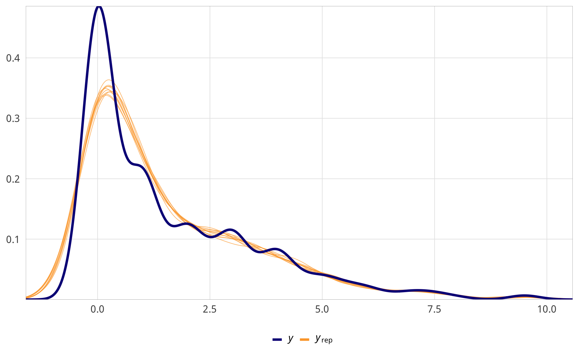

check_total_denom %>% 
  posterior_samples(add_chain = TRUE) %>% 
  select(-starts_with("r_gwcode"), -starts_with("z_"), -lp__, -iter) %>% 
  mcmc_trace() +
  theme_donors() +
  theme(legend.position = "right")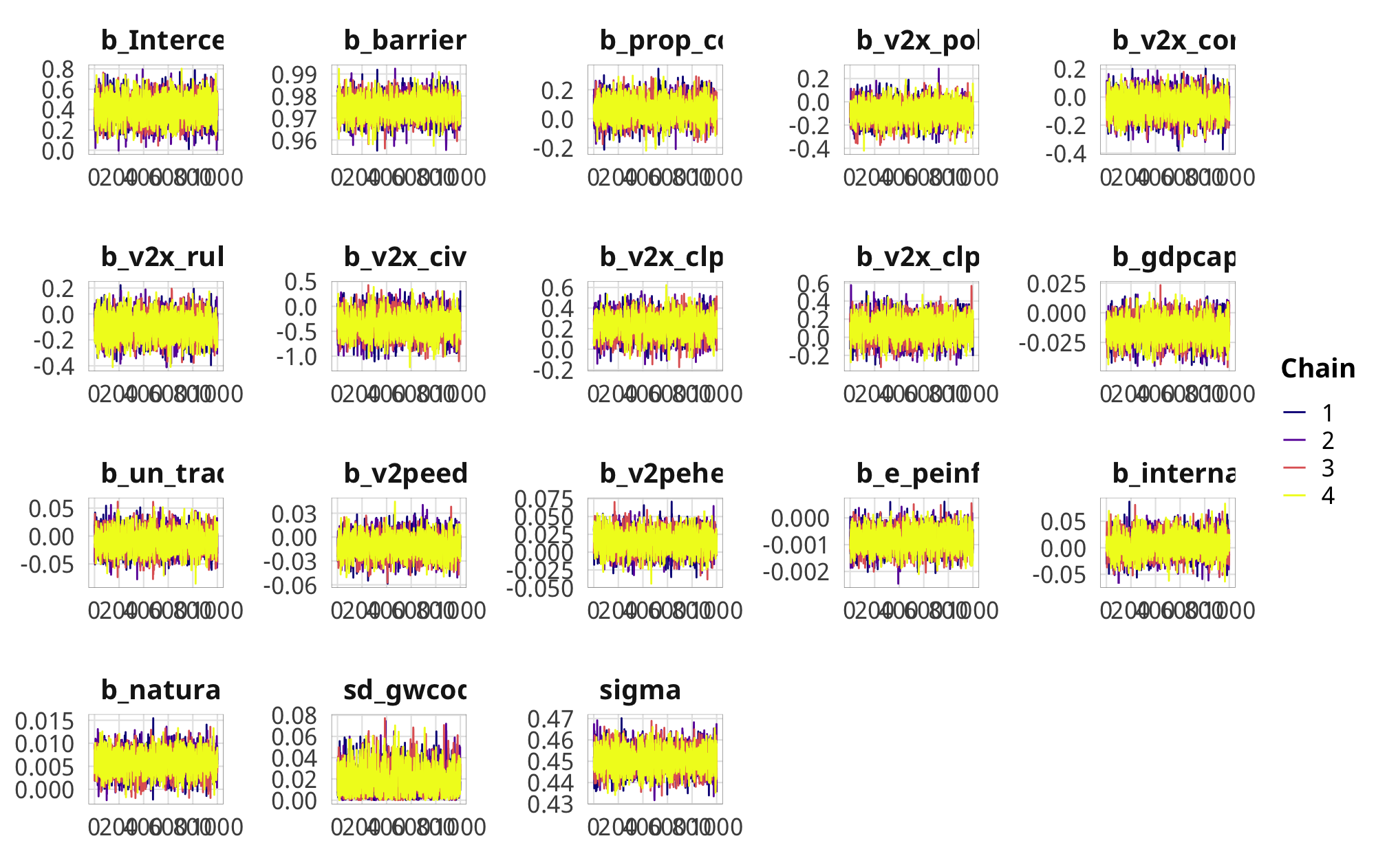

Build weights

tic()
fit_h2_preds <- fit_h2_all_models %>%
  mutate(pred_num = map(fit_num, ~predict(.x, newdata = df_country_aid_laws, allow_new_levels = TRUE)),
         resid_num = map(fit_num, ~residuals(.x, newdata = df_country_aid_laws, allow_new_levels = TRUE)),
         pred_denom = map(fit_denom, ~predict(.x, newdata = df_country_aid_laws, allow_new_levels = TRUE)),
         resid_denom = map(fit_denom, ~residuals(.x, newdata = df_country_aid_laws, allow_new_levels = TRUE)))
toc()

## 108.993 sec elapsed

fit_h2_ipw <- fit_h2_preds %>%
  mutate(num_actual = pmap(list(form = formula_num, pred = pred_num, resid = resid_num), 
                           calc_prob_dist),
         denom_actual = pmap(list(form = formula_denom, pred = pred_denom, resid = resid_denom), 
                          calc_prob_dist)) %>% 
  mutate(df_with_weights = map2(num_actual, denom_actual, ~{
    df_country_aid_laws %>% 
      mutate(weights_sans_time = .x / .y) %>% 
      group_by(gwcode) %>% 
      mutate(ipw = cumprod_na(weights_sans_time)) %>% 
      ungroup()
  }))
fit_h2_ipw

## # A tibble: 4 x 12
##   model_name formula_num formula_denom fit_num fit_denom pred_num resid_num pred_denom
##   <chr>      <list>      <list>        <list>  <list>    <list>   <list>    <list>    
## 1 h2_total   <brmsfrml>  <brmsfrml>    <brmsf… <brmsfit> <dbl[,4… <dbl[,4]… <dbl[,4] …
## 2 h2_advoca… <brmsfrml>  <brmsfrml>    <brmsf… <brmsfit> <dbl[,4… <dbl[,4]… <dbl[,4] …
## 3 h2_entry   <brmsfrml>  <brmsfrml>    <brmsf… <brmsfit> <dbl[,4… <dbl[,4]… <dbl[,4] …
## 4 h2_funding <brmsfrml>  <brmsfrml>    <brmsf… <brmsfit> <dbl[,4… <dbl[,4]… <dbl[,4] …
## # … with 4 more variables: resid_denom <list>, num_actual <list>, denom_actual <list>,
## #   df_with_weights <list>

Outcome models

Modeling choice

Our dependent variable for this hypothesis is the percentage of ODA (still in constant 2011 dollars) allocated for contentious purposes, again leaded by one year. We classify contentious aid as any project focused on government and civil society (DAC codes 150 and 151) or conflict prevention and resolution, peace and security (DAC code 152).

Working with proportion data, however, poses interesting mathematical and methodological challenges, since the range of possible outcomes is limited to a value between 0 and 1. Treating proportion variables in a mixed model is technically possible, but it yields predicitions that go beyond the allowable range of values (1.13, -0.5, etc.). Treating the proportion as a binomial variable is also possible and is indeed one of the ways to use the glm() function in R. However, this entails considering the proportion as a ratio of success and failures. In this case, treating a dollar of contentious aid as a success feels off, especially since aid amounts aren’t independent events—it’s not like each dollar of aid goes through a probabalistic process like a coin flip.

One recommendation by Ben Bolker, the maintainer of lme4, is to use a logit transformation of the dependent variable in lmer() models. This seems to be standard practice in political science research, too. Logit transformations still can’t handle values of exactly 0 or 1, though, but it’s possible to winsorize those values by adding or subtracting 0.001 to the extremes.

Another solution is to use beta regression, which constrains the outcome variable to values between 0 and 1, but unfortunately does not allow for values of exactly 0 or 1. Zero-and-one inflated beta regression models, however, make adjustments for this and model the probability of being 0, being 1, and being somewhere in the middle using different processes. Matti Vuorre has an excellent overview of ZOIB models here.

In the original versions of this project, we used logit-linear models of the ratio of contentious aid to non-contentious aid, like this:

\[ln( \frac{\text{contentious ODA}_{\text{OECD}}}{\text{noncontentious ODA}_{\text{OECD}}} )_{i, t+1} = \text{NGO legislation}_{it} + \text{controls}_{it}\]

That meant we had to compare the ratio of contentious aid to non-contentious aid rather than the direct percent of contentious aid, and it made for some acrobatic interpretations.

Here, we use zero-inflated beta regression instead, since brms and Stan have improved and sped up a ton over the past few years.

The proportion of contentious aid has a bunch of zeroes, and those zeros are close to the distribution of the regular data, so we use zero-inflated models rather than a hurdle process like with did with H₁ and total ODA. Something determines whether a country/year receives any contentious aid, and then something else determines what proportion is contentious.

If we don’t take this zero-inflation process into account in the model, our ATE will be wrong. We don’t really care about the exact zero-inflation process—we care most about the ATE of laws/restrictions on contentiousness—but we still need to deal with the multiple processes.

ggplot(df_country_aid_laws, 
       aes(x = prop_contentious, fill = prop_contentious == 0)) +
  geom_histogram(binwidth = 0.05, color = "white", boundary = 0) +
  labs(x = "Proportion of contentious aid", y = "Count") +
  scale_fill_manual(values = c("grey80", "#FF851B"), 
                    labels = c("% > 0", "% = 0"),
                    name = NULL) +
  scale_x_continuous(labels = percent_format(accuracy = 1)) +
  theme_donors()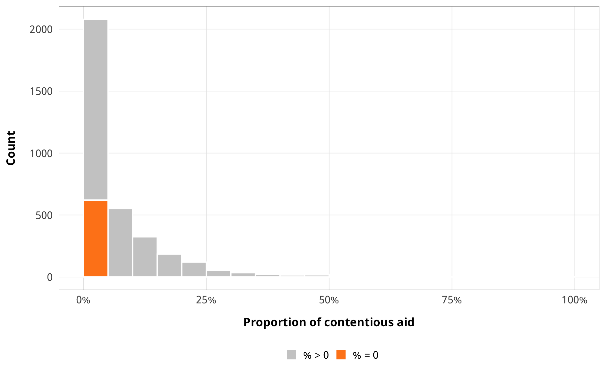

# Percent where prop_contentious is 0:
df_country_aid_laws %>% 
  count(prop_contentious == 0) %>% 
  mutate(prop = n / sum(n))

## # A tibble: 2 x 3
##   `prop_contentious == 0`     n  prop
## * <lgl>                   <int> <dbl>
## 1 FALSE                    2814 0.819
## 2 TRUE                      621 0.181

We thus fit a zero-inflated beta model, which uses a logit model to predict 0/not 0, then uses a beta family to model the rest of the data.

Beta regression is based on the beta distribution and its two shape parameters, but the parameterization of the distribution in brms/stan uses \(\mu\) and \(\phi\), which are transformed versions of shape 1 and shape 2:

• \(\text{shape1} = \mu \phi\)
• \(\text{shape2} = (1 - \mu)\phi\)

This is actually kind of neat, because instead of trying to finagle a beta distribution based on \(\frac{\text{shape1}}{\text{shape1} + \text{shape2}}\), you can specify the average proportion and “spread” similar to a normal distribution.

For instance, if we wanted a beta distribution around 0.3, with some moderate spread, we could play around with shape1 and shape2 and figure that they’re probably something like 3 and 7, based on \(\frac{3}{3 + 7}\). We can get these same numbers with the reparameterized version, using 0.3 as \(\mu\) (i.e. clustered around 0.3) and 10 as \(\phi\). We get the same 3 and 7 values for the two shapes and the distribution looks great! The dprop() function in extraDistr takes these reparameterized arguments directly, too (it calls \(phi\) size).

mu <- 0.3
phi <- 10

shape1 <- mu * phi
shape1

## [1] 3

shape2 <- (1 - mu) * phi
shape2

## [1] 7

# With dbeta
plot_beta <- ggplot() +
  stat_function(fun = dbeta, args = list(shape1 = shape1, shape2 = shape2),
                geom = "area", fill = "grey80", color = "black") +
  scale_x_continuous(labels = percent_format(accuracy = 1)) +
  labs(x = "Proportion", y = NULL, 
       title = "Beta distribution",
       subtitle = glue("shape1 = {shape1}; shape2 = {shape2}")) +
  theme_donors(9) +
  theme(axis.text.y = element_blank())

# With dprop
plot_prop <- ggplot() +
  stat_function(fun = dprop, args = list(size = phi, mean = mu),
                geom = "area", fill = "grey80", color = "black") +
  scale_x_continuous(labels = percent_format(accuracy = 1)) +
  labs(x = "Proportion", y = NULL, 
       title = "Reparameterized beta distribution",
       subtitle = glue("µ = {mu}; φ = {phi}")) +
  theme_donors(9) +
  theme(axis.text.y = element_blank())

plot_beta + plot_prop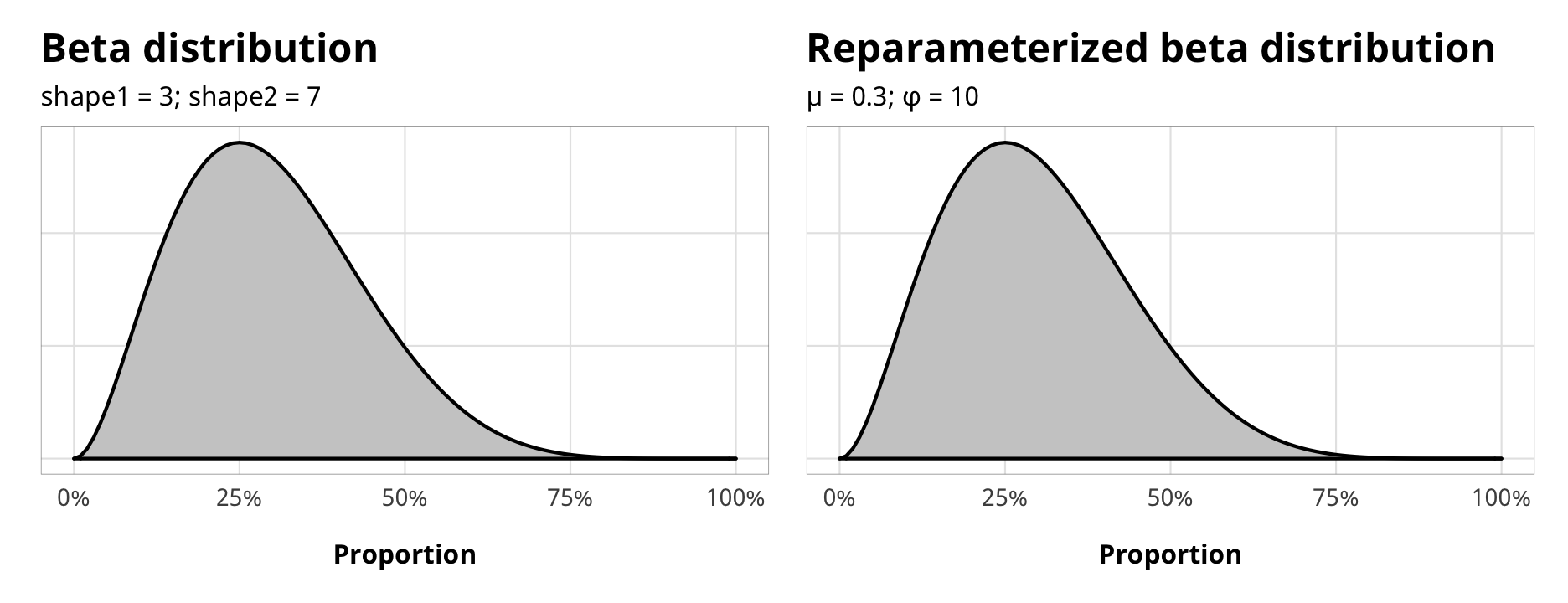

The median proportion of contentious aid for non-zero cases is around 5%, and based on the histogram earlier, it’s not unheard of to go up to 25% or even as high as 50%:

df_country_aid_laws %>% 
  filter(prop_contentious > 0) %>% 
  summarize(median_prop = median(prop_contentious))

## # A tibble: 1 x 1
##   median_prop
##         <dbl>
## 1      0.0466

In the absence of any covariates, we could use a \(mu\) of 0.05 and a \(phi\) of 3:

beta_mu <- 0.05
beta_phi <- 3

# beta_shape1 <- beta_mu * beta_phi
# beta_shape2 <- (1 - beta_mu) * beta_phi

ggplot() +
  stat_function(fun = dprop, args = list(size = beta_phi, mean = beta_mu),
                geom = "area", fill = "grey80", color = "black") +
  scale_x_continuous(labels = percent_format(accuracy = 1)) +
  labs(x = "Proportion", y = NULL, 
       title = "Reparameterized beta distribution",
       subtitle = glue("µ = {beta_mu}; φ = {beta_phi}")) +
  theme_donors(9) +
  theme(axis.text.y = element_blank())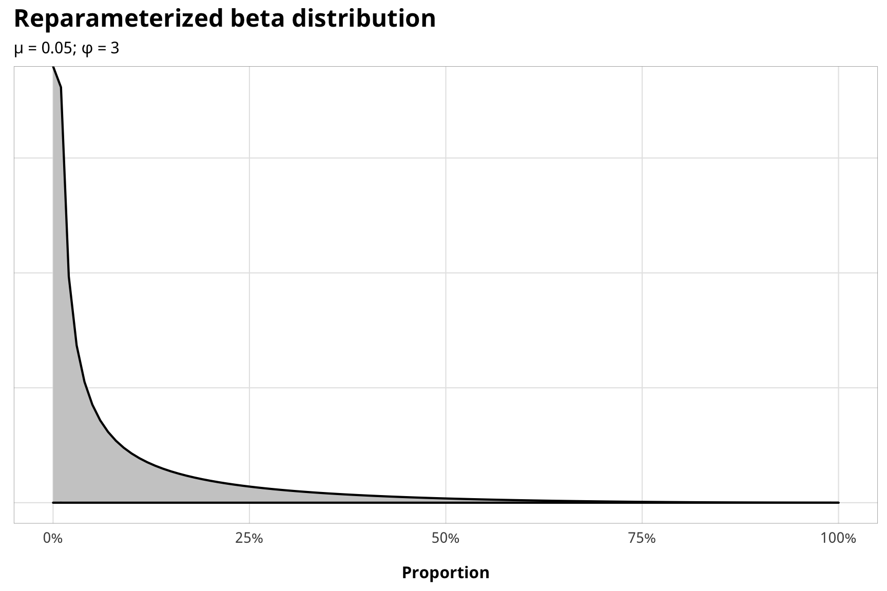

This gets more complex, though, once we start adding covariates. \(\mu\) is modeled with logistic regression while \(\phi\) is modeled with a log link, and each of these models can get their own covariates.

Priors for outcome models

There are a ton of moving parts in these outcome models. Here’s the full specification for the models and all priors:

\[ \begin{aligned} \text{y}_{i,t} | u_i, \text{Law}_{i, t} &\sim \operatorname{ZIBeta} (Z_i, \text{y}^\star_i, \phi_i) & \text{[likelihood]} \\ \operatorname{logit} (Z_i) &\sim \alpha_Z & \text{[intercept-only logit if } \text{y}_{i, t} = 0 \text{]} \\ \operatorname{logit} (\text{y}^\star_i) &\sim (\beta_0 + \beta_1 \text{Law}_{i, t} + \beta_2 \text{Law}_{i, t-1}, \sigma^2_\epsilon, u_i) \times \text{IPW}_{i, t} & \text{[if } \text{y}_{i, t} > 0 \text{]}\\ \log (\phi_i) &\sim \alpha_\phi & \text{[intercept-only model for precision]} \\ u_i &\sim \mathcal{N} (0, \sigma^2_u) & \text{[country-specific intercepts]} \\ \ \\ \alpha_Z &\sim \operatorname{Logistic}(-1.5, 0.5) & \text{[prior proportion of rows where y = 0]} \\ \alpha_\phi &\sim \operatorname{Gamma} (0.01, 0.01) & \text{[prior Beta precision]} \\ \beta_0 &\sim \mathcal{N} (0, 10) & \text{[prior population intercept]} \\ \beta_1, \beta_2 &\sim \mathcal{N} (0, 3) & \text{[prior population effects]} \\ \sigma^2_e, \sigma^2_u &\sim \operatorname{Cauchy}(0, 1) & \text{[prior sd for population and country]} \\ \ \\ \text{IPW}_{i, t} &= \prod^t_{t = 1} \frac{\phi(T_{it} | T_{i, t-1}, C_i)}{\phi(T_{it} | T_{i, t-1}, D_{i, t-1}, C_i)} & \text{[stabilized weights]} \end{aligned} \] For \(\phi\), we just use Stan’s default Gamma(0.01, 0.01). Here’s what all these prior distributions look like:

z_p <- ggplot() +
  stat_function(fun = dlogis, args = list(location = -1.5, scale = 0.5),
                geom = "area", fill = "grey80", color = "black") +
  labs(x = TeX("\\textbf{Prop. contentious = 0 (α_Z)}")) +
  annotate(geom = "label", x = -2, y = 0.07, label = "Logistic(-1.5, 0.5)", size = pts(9)) +
  xlim(-8, 3) +
  theme_donors(prior = TRUE)

b0_p <- ggplot() +
  stat_function(fun = dnorm, args = list(mean = 0, sd = 10),
                geom = "area", fill = "grey80", color = "black") +
  labs(x = TeX("\\textbf{Population intercept (β_0)}")) +
  annotate(geom = "label", x = 0, y = 0.0042, label = "N(0, 10)", size = pts(9)) +
  xlim(-40, 40) +
  theme_donors(prior = TRUE)

b12_p <- ggplot() +
  stat_function(fun = dnorm, args = list(mean = 0, sd = 3),
                geom = "area", fill = "grey80", color = "black") +
  labs(x = TeX("\\textbf{Population effects (β_1, β_2)}")) +
  annotate(geom = "label", x = 0, y = 0.02, label = "N(0, 3)", size = pts(9)) +
  xlim(-10, 10) +
  theme_donors(prior = TRUE)

sigma_p <- ggplot() +
  stat_function(fun = dcauchy, args = list(location = 0, scale = 1),
                geom = "area", fill = "grey80", color = "black") +
  labs(x = TeX("\\textbf{Population and country SD (σ_e, σ_u)}")) +
  annotate(geom = "label", x = 5, y = 0.04, label = "Cauchy(0, 1)", size = pts(9)) +
  xlim(0, 10) +
  theme_donors(prior = TRUE)

phi_p <- ggplot() +
  stat_function(fun = dgamma, args = list(shape = 0.1, scale = 0.1),
                geom = "area", fill = "grey80", color = "black") +
  labs(x = TeX("\\textbf{Beta precision (φ)}")) +
  annotate(geom = "label", x = 0.25, y = 2, label = "Gamma(0.01, 0.01)", size = pts(9)) +
  xlim(0, 0.5) +
  theme_donors(prior = TRUE)

layout <- "
AAAABBBBCCCC
AAAABBBBCCCC
##DDDDEEEE##
##DDDDEEEE##
"
z_p + sigma_p + phi_p + b0_p + b12_p +
  plot_layout(design = layout)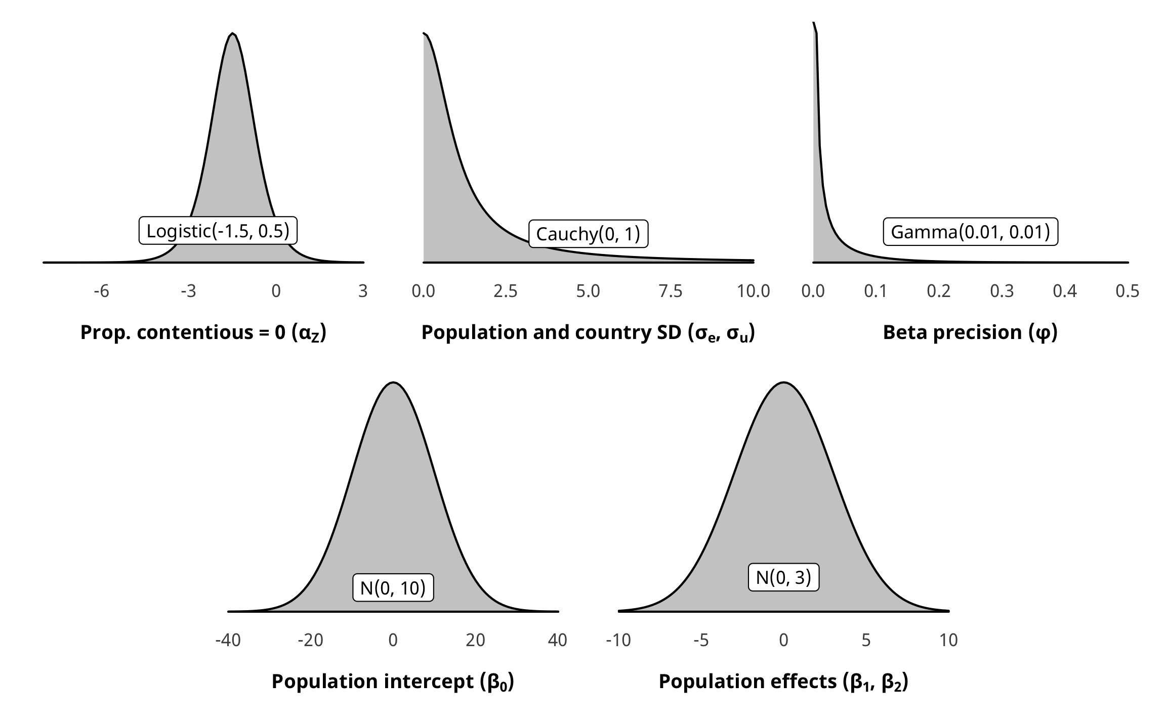

As with H₁, the prior for the zero-inflated part of the model is a little weird. Internally, Stan uses a default of logistic(0, 1). We want to use an informative beta(1.8, 8,1) prior that approximates the proportion of zeroes in the data (but with fairly wide dispersion), but we once again need to translate it into the logistic distribution. Since there’s no easy way to do this, we used brms::logit_scaled to play around with distributional hyperparameters until it looked okay in the logistic distribution.

zi_prior_sim <- tibble(beta = rbeta(10000, 1.8, 8.1)) %>% 
  mutate(beta_logit_scale = brms::logit_scaled(beta)) %>% 
  mutate(logit_betaish_prior = rlogis(10000, -1.5, 0.5)) %>% 
  mutate(prior_probs = plogis(logit_betaish_prior))

zi_prior_plot1 <- ggplot(zi_prior_sim) +
  geom_density(aes(x = beta), fill = "grey80", color = "black") +
  labs(x = "Proportion where prop. contentious = 0",
       subtitle = "Original Beta(1.8, 8.1) distribution") +
  coord_cartesian(xlim = c(0, 1)) +
  theme_donors(prior = TRUE)

zi_prior_plot2 <- ggplot(zi_prior_sim) +
  geom_density(aes(x = beta_logit_scale), fill = "grey80", color = "black") +
  labs(x = "Logistic value where prop. contentious = 0",
       subtitle = "Beta(1.8, 8.1) scaled with brms::logit_scaled") +
  coord_cartesian(xlim = c(-8, 1)) +
  theme_donors(prior = TRUE)

zi_prior_plot3 <- ggplot(zi_prior_sim) +
  geom_density(aes(x = logit_betaish_prior), fill = "grey80", color = "black") +
  labs(x = "Logistic value where prop. contentious = 0",
       subtitle = "Estimated Logistic(-1.5, 0.5)") +
  coord_cartesian(xlim = c(-8, 1)) +
  theme_donors(prior = TRUE)

zi_prior_plot4 <- ggplot(zi_prior_sim) +
  geom_density(aes(x = prior_probs), fill = "grey80", color = "black") +
  labs(x = "Proportion where prop. contentious = 0",
       subtitle = "Logistic(-1.5, 0.5) transformed to probabilities") +
  coord_cartesian(xlim = c(0, 1)) +
  theme_donors(prior = TRUE)

(zi_prior_plot1 + zi_prior_plot2) / (zi_prior_plot3 + zi_prior_plot4)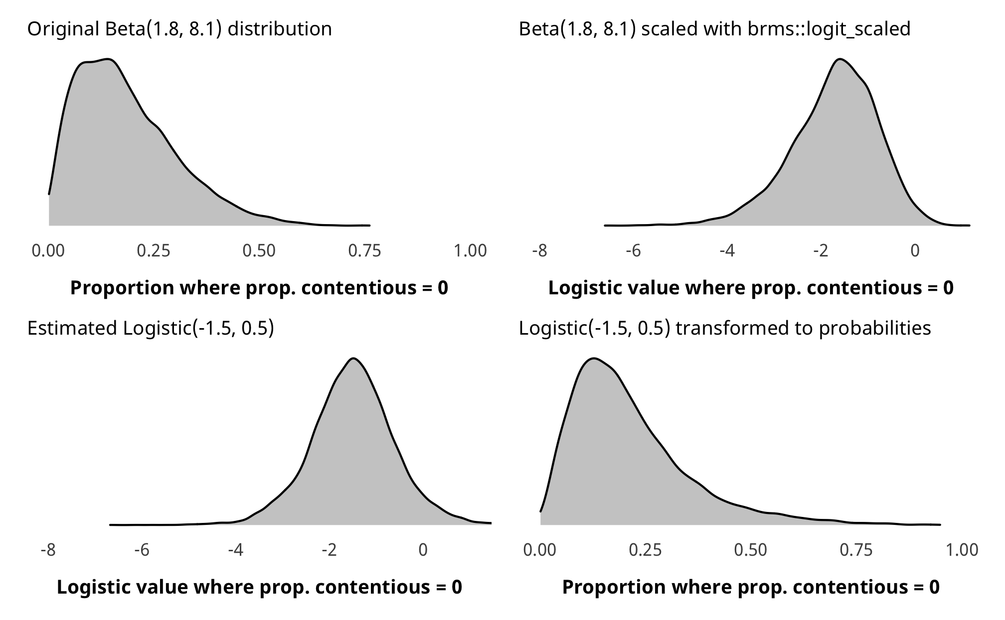

Run outcome models

Outcome model time!

# Outcome -----------------------------------------------------------------
# Formulas
# Treatment ~ lag treatment + non-varying confounders
formula_h2_out_total <- bf(prop_contentious_lead1 | weights(ipw) ~ 
                             barriers_total + (1 | gwcode),
                           zi ~ 1)
formula_h2_out_advocacy <- bf(prop_contentious_lead1 | weights(ipw) ~ 
                                advocacy + (1 | gwcode),
                              zi ~ 1)
formula_h2_out_entry <- bf(prop_contentious_lead1 | weights(ipw) ~ 
                             entry + (1 | gwcode),
                           zi ~ 1)
formula_h2_out_funding <- bf(prop_contentious_lead1 | weights(ipw) ~ 
                               funding + (1 | gwcode),
                             zi ~ 1)

# Priors
prior_out <- c(set_prior("normal(0, 10)", class = "Intercept"),
               set_prior("normal(0, 3)", class = "b"),
               set_prior("cauchy(0, 1)", class = "sd"),
               set_prior("logistic(-1.5, 0.5)", class = "Intercept", dpar = "zi"),
               set_prior("gamma(0.01, 0.01)", class = "phi"))

# Run outcome models ------------------------------------------------------
tic()
fit_h2_outcomes <- fit_h2_ipw %>%
  mutate(formula_outcome = 
           list(formula_h2_out_total, formula_h2_out_advocacy, 
                formula_h2_out_entry, formula_h2_out_funding)) %>% 
  mutate(fit_outcome = 
           pmap(list(formula_outcome, df_with_weights, model_name),
                ~brm(
                  ..1,
                  data = ..2,
                  prior = prior_out,
                  family = zero_inflated_beta(),
                  iter = ITER * 2, chains = CHAINS, warmup = WARMUP, seed = BAYES_SEED,
                  file = here("analysis", "model_cache", paste0(..3, "_outcome.rds"))
                )))
fit_h2_outcomes
toc()

Check outcome models

check_total_outcome <- fit_h2_outcomes %>% 
  filter(model_name == "h2_total") %>% pull(fit_outcome) %>% first()

pp_check(check_total_outcome, type = "dens_overlay", nsamples = 10) +
  scale_x_continuous(labels = percent_format(accuracy = 1)) +
  theme_donors()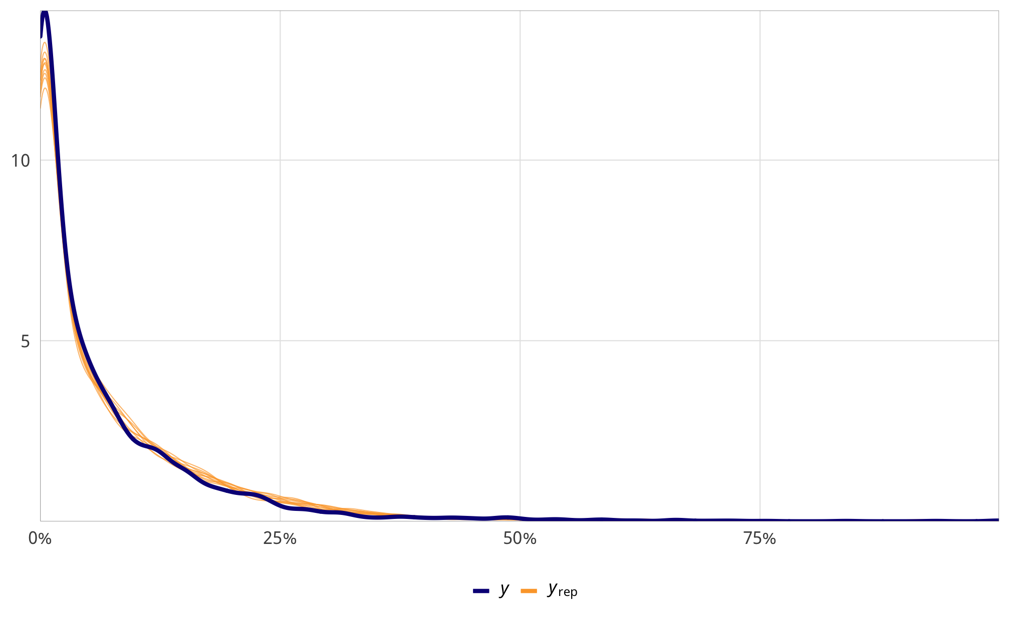

check_total_outcome %>% 
  posterior_samples(add_chain = TRUE) %>% 
  select(-starts_with("r_gwcode"), -starts_with("z_"), -lp__, -iter) %>% 
  mcmc_trace() +
  theme_donors()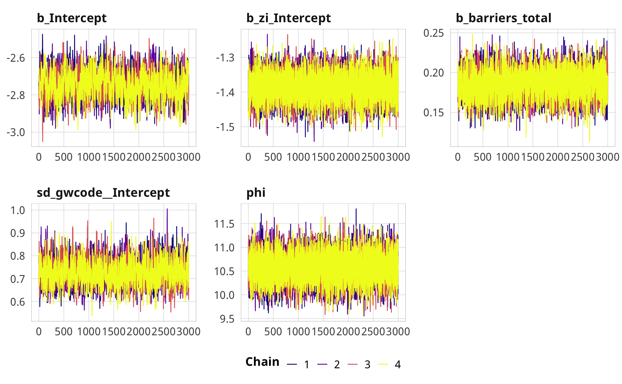

Results

# Plots!
plot_total <- fit_h2_outcomes %>% 
  filter(model_name == "h2_total") %>% 
  pull(fit_outcome) %>% nth(1) %>% 
  gather_draws(b_barriers_total) %>%
  mutate(.value = exp(.value) - 1) %>% 
  mutate(.variable = dplyr::recode(.variable, 
                                   b_barriers_total = "Additional law, t - 1")) %>% 
  ggplot(aes(y = fct_rev(.variable), x = .value, fill = fct_rev(.variable))) +
  geom_vline(xintercept = 0) +
  stat_halfeye(.width = c(0.8, 0.95), alpha = 0.8) +
  guides(fill = FALSE) +
  scale_x_continuous(labels = percent_format(accuracy = 1)) +
  scale_fill_manual(values = c("#FF851B", "#FFDC00")) +
  labs(y = NULL, x = NULL) +
  theme_donors()

plot_advocacy <- fit_h2_outcomes %>% 
  filter(model_name == "h2_advocacy") %>% 
  pull(fit_outcome) %>% nth(1) %>% 
  gather_draws(b_advocacy) %>% 
  mutate(.variable = dplyr::recode(.variable, 
                                   b_advocacy = "Additional advocacy law, t - 1")) %>% 
  mutate(.value = exp(.value) - 1) %>% 
  ggplot(aes(y = fct_rev(.variable), x = .value, fill = fct_rev(.variable))) +
  geom_vline(xintercept = 0) +
  stat_halfeye(.width = c(0.8, 0.95), alpha = 0.8) +
  guides(fill = FALSE) +
  scale_x_continuous(labels = percent_format(accuracy = 1)) +
  scale_fill_manual(values = c("#85144b", "#F012BE")) +
  labs(y = NULL, x = NULL) +
  theme_donors()

plot_entry <- fit_h2_outcomes %>% 
  filter(model_name == "h2_entry") %>% 
  pull(fit_outcome) %>% nth(1) %>% 
  gather_draws(b_entry) %>% 
  mutate(.variable = dplyr::recode(.variable, 
                                   b_entry = "Additional entry law, t - 1")) %>% 
  mutate(.value = exp(.value) - 1) %>% 
  ggplot(aes(y = fct_rev(.variable), x = .value, fill = fct_rev(.variable))) +
  geom_vline(xintercept = 0) +
  stat_halfeye(.width = c(0.8, 0.95), alpha = 0.8) +
  guides(fill = FALSE) +
  scale_x_continuous(labels = percent_format(accuracy = 1)) +
  scale_fill_manual(values = c("#3D9970", "#2ECC40")) +
  labs(y = NULL, x = "% change in proportion of contentious aid") +
  theme_donors()

plot_funding <- fit_h2_outcomes %>% 
  filter(model_name == "h2_funding") %>% 
  pull(fit_outcome) %>% nth(1) %>% 
  gather_draws(b_funding) %>% 
  mutate(.variable = dplyr::recode(.variable, 
                                   b_funding = "Additional funding law, t - 1")) %>% 
  mutate(.value = exp(.value) - 1) %>% 
  ggplot(aes(y = fct_rev(.variable), x = .value, fill = fct_rev(.variable))) +
  geom_vline(xintercept = 0) +
  stat_halfeye(.width = c(0.8, 0.95), alpha = 0.8) +
  guides(fill = FALSE) +
  scale_x_continuous(labels = percent_format(accuracy = 1)) +
  scale_fill_manual(values = c("#001f3f", "#0074D9")) +
  labs(y = NULL, x = "% change in proportion of contentious aid") +
  theme_donors()

(plot_total + plot_advocacy) / (plot_entry + plot_funding)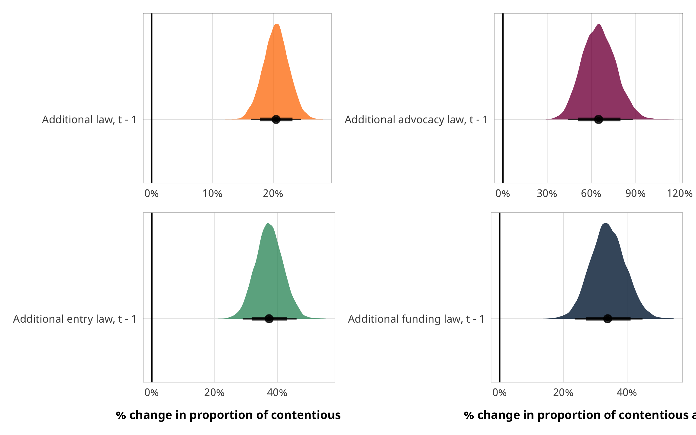

A one-unit change in X results in a relative change of \(e^\beta\) in \(\frac{\text{E(Proportion)}}{1 - \text{E(Proportion)}}\) - see https://stats.stackexchange.com/questions/297659/interpretation-of-betareg-coef - the ratio of contentious to non-contentious aid? the ratio of of contentious aid?

See also https://stats.stackexchange.com/a/230679/3025 and https://static1.squarespace.com/static/58a7d1e52994ca398697a621/t/5a2ebc43e4966b0fab6b02de/1513012293857/betareg_politics.pdf

fit_h2_outcomes %>% 
  filter(model_name == "h2_total") %>% 
  pull(fit_outcome) %>% nth(1) %>% 
  conditional_effects()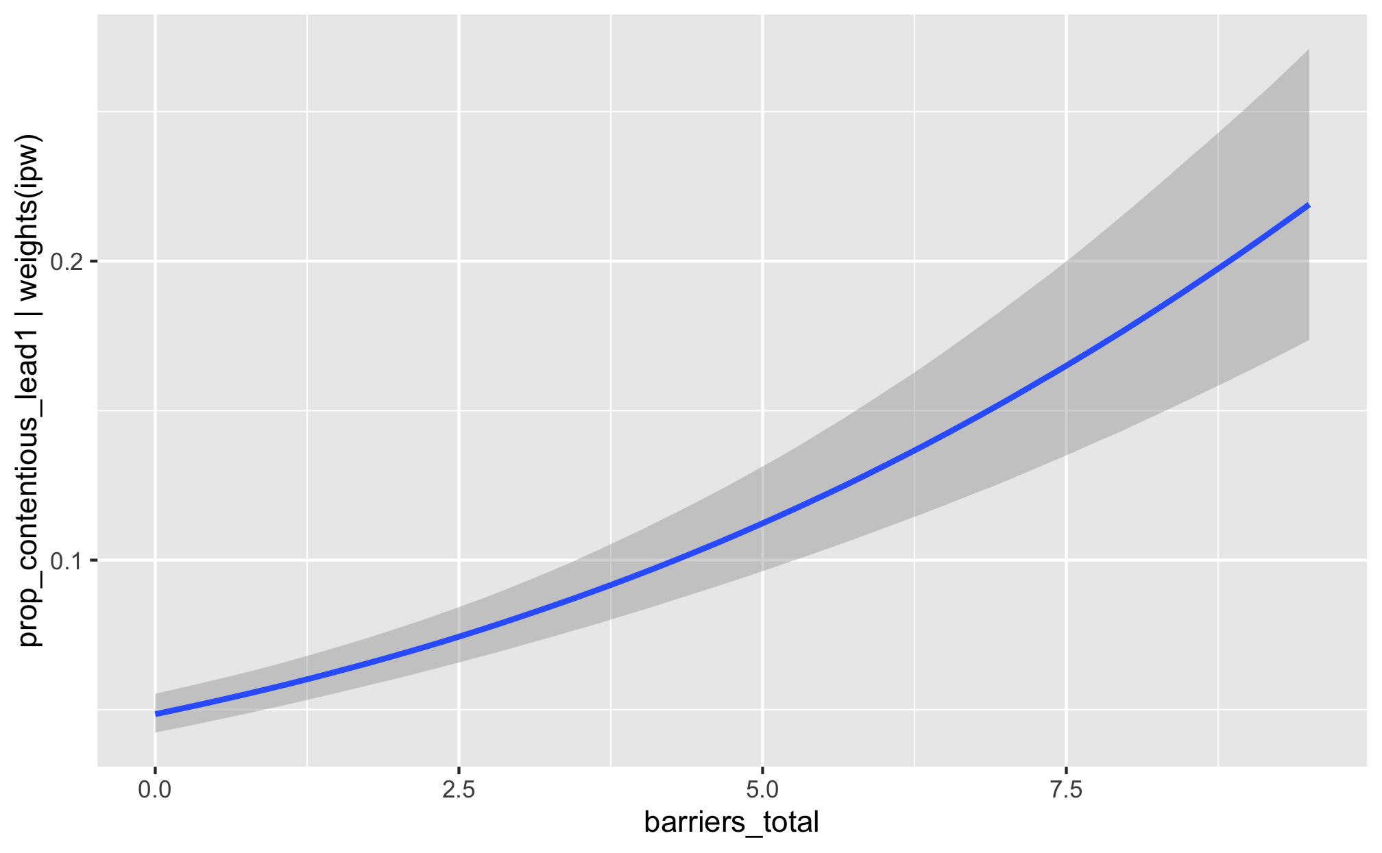

fit_h2_outcomes %>% 
  filter(model_name == "h2_advocacy") %>% 
  pull(fit_outcome) %>% nth(1) %>% 
  conditional_effects()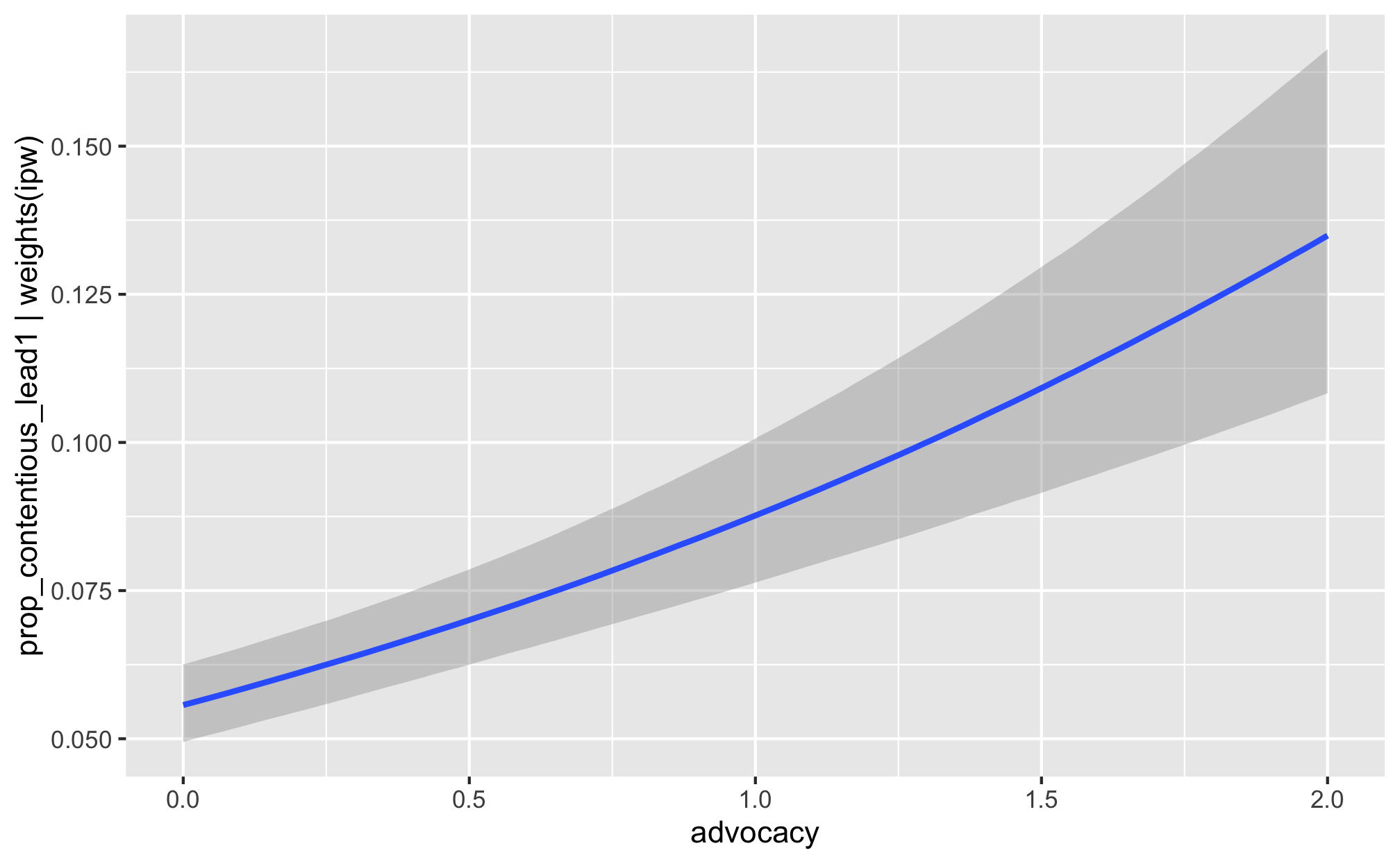

fit_h2_outcomes %>% 
  filter(model_name == "h2_entry") %>% 
  pull(fit_outcome) %>% nth(1) %>% 
  conditional_effects()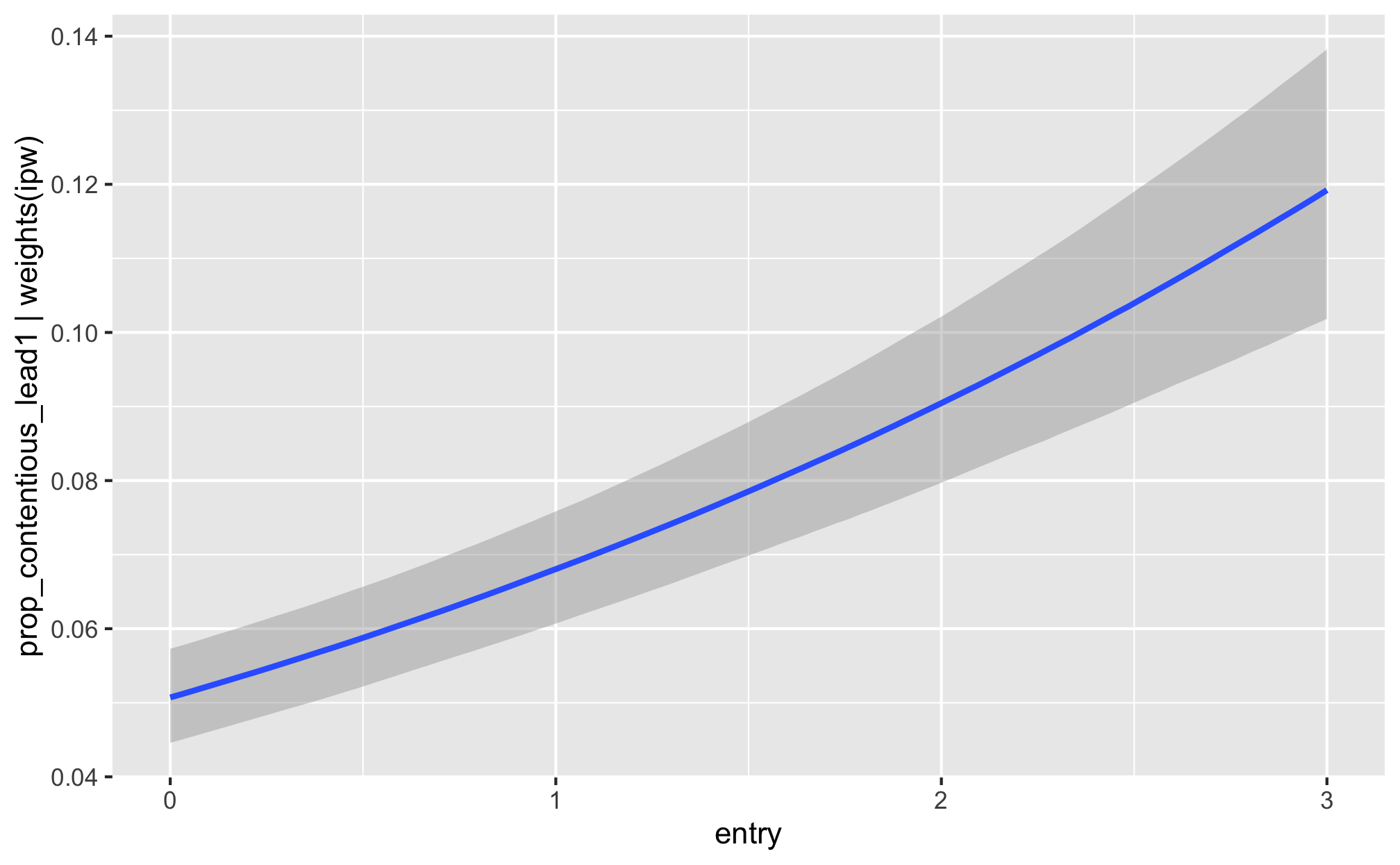

fit_h2_outcomes %>% 
  filter(model_name == "h2_funding") %>% 
  pull(fit_outcome) %>% nth(1) %>% 
  conditional_effects()

Copyright © 2017–2021 Suparna Chaudhry and Andrew Heiss. Licensed under the MIT License. Code available on GitHub.