Process and merge data
Suparna Chaudhry and Andrew Heiss
Last run: 2021-03-14
library(tidyverse)
library(countrycode)
library(states)
library(WDI)
library(haven)
library(readxl)
library(naniar)
library(lubridate)
library(scales)
library(xml2)
library(httr)
library(rvest)
library(DT)
library(pander)
library(here)
Load raw data
# V-Dem
vdem_raw <- read_rds(here("data", "raw_data", "Country_Year_V-Dem_Full+others_R_v10",
                         "V-Dem-CY-Full+Others-v10.rds")) %>% as_tibble()

# World Bank World Development Indicators (WDI)
# http://data.worldbank.org/data-catalog/world-development-indicators
wdi_indicators <- c("NY.GDP.PCAP.PP.KD",  # GDP per capita, ppp (constant 2011 international $)
                    "NY.GDP.MKTP.PP.KD",  # GDP, ppp (constant 2010 international $)
                    "NE.TRD.GNFS.ZS",  # Trade (% of GDP)
                    "SP.POP.TOTL")     # Population, total

wdi_raw <- WDI(country = "all", wdi_indicators, extra = TRUE, start = 1980, end = 2018)

# Chaudhry restrictions
# In this data Sudan (625) splits into North Sudan (626) and South Sudan (525)
# in 2011, but in the other datasets regular Sudan stays 625 and South Sudan
# becomes 626, so adjust the numbers here
#
# Also, Chad is in the dataset, but all values are missing, so we drop it
chaudhry_raw <- read_dta(here("data", "raw_data",
                              "Chaudhry restrictions", "SC_Expanded.dta")) %>%
  filter(ccode != 483) %>%  # Remove Chad
  mutate(ccode = case_when(
    scode == "SSU" ~ 626,
    scode == "SDN" ~ 625,
    TRUE ~ ccode
  )) %>%
  mutate(gwcode = countrycode(ccode, origin = "cown", destination = "gwn",
                              custom_match = c("679" = 678L, "818" = 816L,
                                               "342" = 345L, "341" = 347L,
                                               "348" = 341L, "315" = 316L)))

# UCDP/PRIO Armed Conflict
ucdp_prio_raw <- read_csv(here("data", "raw_data", "UCDP PRIO",
                               "ucdp-prio-acd-191.csv"))
Create country-year skeleton
We use Gleditsch-Ward country codes to identify each country across the different datasets we merge. We omit microstates.
Importantly, when converting GW codes to COW codes, following Gleditsch and Ward, we treat post-2006 Serbia as 345 (a continuation of Serbia & Montenegro). And we also treat Serbia as a continuation of Yugoslavia with 345 (following V-Dem, which does that too).
In both COW and GW codes, modern Vietnam is 816, but countrycode() thinks the COW code is 817, which is old South Vietnam (see issue), so we use custom_match to force 816 to recode to 816.
Also, following Gleditsch and Ward, we treat Serbia after 2006 dissolution of Serbia & Montenegro as 345 in COW codes (see here)
Also, following V-Dem, we treat Czechoslovakia (GW/COW 315) and Czech Republic (GW/COW 316) as the same continuous country (V-Dem has both use ID 157).
Also, because the World Bank doesn’t include it in the WDI, we omit Taiwan (713). We also omit East Germany (265) and South Yemen (680).
microstates <- gwstates %>%
  filter(microstate) %>% distinct(gwcode, iso3c)

panel_skeleton_all <- state_panel(1980, 2018, partial = "any") %>%
  mutate(year = year(date)) %>%
  filter(!(gwcode %in% microstates$gwcode)) %>%
  filter(!(gwcode %in% c(265, 680, 713))) %>%
  mutate(gwcode = recode(gwcode, `315` = 316L)) %>%
  mutate(cowcode = countrycode(gwcode, origin = "gwn", destination = "cown",
                               custom_match = c("816" = 816L, "340" = 345L)),
         country = countrycode(cowcode, origin = "cown", destination = "country.name",
                               custom_match = c("678" = "Yemen")),
         iso2 = countrycode(cowcode, origin = "cown", destination = "iso2c",
                            custom_match = c("345" = "RS", "347" = "XK", "678" = "YE")),
         iso3 = countrycode(cowcode, origin = "cown", destination = "iso3c",
                            custom_match = c("345" = "SRB", "347" = "XKK", "678" = "YEM")),
         # Use 999 as the UN country code for Kosovo
         un = countrycode(cowcode, origin = "cown", destination = "un",
                          custom_match = c("345" = 688, "347" = 999, "678" = 887))) %>%
  # There are two entries for "Yugoslavia" in 2006 after recoding 340 as 345;
  # get rid of one
  filter(!(gwcode == 340 & cowcode == 345 & year == 2006)) %>%
  # Remove the Bahamas, Belize, and Brunei
  filter(!(gwcode %in% c(31, 80, 835))) %>%
  # Make Serbia 345 in GW codes too, for joining with other datasets
  mutate(gwcode = recode(gwcode, `340` = 345L)) %>%
  select(-date) %>%
  arrange(gwcode, year)
But, we’re ultimately not using all 170 of those countries. There are 163 countries in Suparna’s anti-NGO law data, so we’re limiting the analysis to just those.
Additionally, we exclude long-term consolidated democracies from our analysis, following FinkelPerez-LinanSeligson:2007, 414. These are classified by the World Bank as high income; they score below 3 on Freedom House’s Scale, receive no aid from USAID, and are not newly independent states:
consolidated_democracies <-
  tibble(country_name = c("Andorra", "Australia", "Austria", "Bahamas",
                          "Barbados", "Belgium", "Canada", "Denmark", "Finland",
                          "France", "Germany", "Greece", "Grenada", "Iceland",
                          "Ireland", "Italy", "Japan", "Liechtenstein", "Luxembourg",
                          "Malta", "Monaco", "Netherlands", "New Zealand", "Norway",
                          "San Marino", "Spain", "Sweden", "Switzerland",
                          "United Kingdom", "United States of America")) %>%
  # Ignore these 5 microstates, since they're not in the panel skeleton
  filter(!(country_name %in% c("Andorra", "Grenada", "Liechtenstein",
                               "Monaco", "San Marino"))) %>%
  mutate(iso3 = countrycode(country_name, "country.name", "iso3c"),
         gwcode = countrycode(country_name, "country.name", "gwn"))

consolidated_democracies %>% knitr::kable()| country_name | iso3 | gwcode |
|---|---|---|
| Australia | AUS | 900 |
| Austria | AUT | 305 |
| Bahamas | BHS | 31 |
| Barbados | BRB | 53 |
| Belgium | BEL | 211 |
| Canada | CAN | 20 |
| Denmark | DNK | 390 |
| Finland | FIN | 375 |
| France | FRA | 220 |
| Germany | DEU | 260 |
| Greece | GRC | 350 |
| Iceland | ISL | 395 |
| Ireland | IRL | 205 |
| Italy | ITA | 325 |
| Japan | JPN | 740 |
| Luxembourg | LUX | 212 |
| Malta | MLT | 338 |
| Netherlands | NLD | 210 |
| New Zealand | NZL | 920 |
| Norway | NOR | 385 |
| Spain | ESP | 230 |
| Sweden | SWE | 380 |
| Switzerland | CHE | 225 |
| United Kingdom | GBR | 200 |
| United States of America | USA | 2 |
Thus, here’s our actual panel skeleton:
chaudhry_countries <- chaudhry_raw %>% distinct(gwcode)

panel_skeleton <- panel_skeleton_all %>%
  filter(gwcode %in% chaudhry_countries$gwcode) %>%
  filter(!(gwcode %in% consolidated_democracies$gwcode))

skeleton_lookup <- panel_skeleton %>%
  group_by(gwcode, cowcode, country, iso2, iso3, un) %>%
  summarize(years_included = n()) %>%
  ungroup() %>%
  arrange(country)
We have 142 countries in this data, spanning 39 possible years. Here’s a lookup table of all the countries included:
skeleton_lookup %>%
  datatable()
Foreign aid
OECD and AidData
The OECD collects detailed data on all foreign aid flows (ODA) from OECD member countries (and some non-member countries), mulilateral organizations, and the Bill and Melinda Gates Foundation (for some reason they’re the only nonprofit donor) to all DAC-eligible countries (and some non non-DAC-eligible countries).
The OECD tracks all this in a centralized Creditor Reporting System database and provides a nice front end for it at OECD.Stat with an open (but inscrutable) API (raw CRS data is also available). There are a set of pre-built queries with information about ODA flows by donor, recipient, and sector (purpose), but the pre-built data sources do not include all dimensions of the data. For example, Table DAC2a includes columns for donor, recipient, year, and total ODA (e.g. the US gave $X to Nigeria in 2008) , but does not indicate the purpose/sector for the ODA. Table DAC5 includes columns for the donor, sector, year, and total ODA (e.g. the US gave $X for education in 2008), but does not include recipient information.
Instead of using these pre-built queries or attempting to manipulate their parameters, it’s possible to use the OECD’s QWIDS query builder to create a custom download of data. However, it is slow and clunky and requires significant munging and filtering after exporting.
The solution to all of this is to use data from AidData, which imports raw data from the OECD, cleans it, verifies it, and makes it freely available on GitHub.
AidData offers multiple versions of the data, including a full release, a thin release, aggregated donor/recipient/year data, and aggregated donor/recipient/year/purpose data. For the purposes of this study, all we care about are ODA flows by donor, recipient, year, and purpose, which is one of the ready-made datasets.
Notably, this aggregated data shows total aid commitments, not aid disbursements. Both types of ODA information are available from the OECD and it’s possible to get them using OECD’s raw data. However, AidData notes that disbursement data is sticky and slow—projects take a long time to fulfill and actual inflows of aid in a year can be tied to commitments made years before. Because we’re interested in donor reactions to restrictions on NGOs, any reaction would be visible in the decision to commit money to aid, not in the ultimate disbursement of aid, which is most likely already legally obligated and allocated to the country regardless of restrictions.
So, we look at ODA commitments.
aiddata_url <- "https://github.com/AidData-WM/public_datasets/releases/download/v3.1/AidDataCore_ResearchRelease_Level1_v3.1.zip"
aiddata_path <- here("data", "raw_data", "AidData")
aiddata_zip_name <- basename(aiddata_url)
aiddata_name <- tools::file_path_sans_ext(aiddata_zip_name)

aiddata_final_name <- "AidDataCoreDonorRecipientYearPurpose_ResearchRelease_Level1_v3.1.csv"

# Download AidData data if needed
if (!file.exists(file.path(aiddata_path, aiddata_final_name))) {
  aiddata_get <- GET(aiddata_url,
                     write_disk(file.path(aiddata_path, aiddata_zip_name),
                                overwrite = TRUE),
                     progress())
  unzip(file.path(aiddata_path, aiddata_zip_name), exdir = aiddata_path)

  # Clean up zip file and unnecessary CSV files
  file.remove(file.path(aiddata_path, aiddata_zip_name))
  list.files(aiddata_path, pattern = "csv", full.names = TRUE) %>%
    map(~ ifelse(str_detect(.x, "DonorRecipientYearPurpose"), 0,
                 file.remove(file.path(.x))))
}

# Clean up AidData data
aidraw_data <- read_csv(file.path(aiddata_path, aiddata_final_name))

aiddata_clean <- aidraw_data %>%
  # Get rid of non-country recipients
  filter(!str_detect(recipient,
                     regex("regional|unspecified|multi|value|global|commission",
                           ignore_case = TRUE))) %>%
  filter(year < 9999) %>%
  mutate(purpose_code_short = as.integer(str_sub(coalesced_purpose_code, 1, 3)))

# Donor, recipient, and purpose details
# I pulled these country names out of the dropdown menu at OECD.Stat Table 2a
# online: https://stats.oecd.org/Index.aspx?DataSetCode=Table2A
dac_donors <- c("Australia", "Austria", "Belgium", "Canada", "Czech Republic",
                "Denmark", "Finland", "France", "Germany", "Greece", "Iceland",
                "Ireland", "Italy", "Japan", "Korea", "Luxembourg", "Netherlands",
                "New Zealand", "Norway", "Poland", "Portugal", "Slovak Republic",
                "Slovenia", "Spain", "Sweden", "Switzerland", "United Kingdom",
                "United States")

non_dac_donors <- c("Bulgaria", "Croatia", "Cyprus", "Estonia", "Hungary",
                    "Israel", "Kazakhstan", "Kuwait", "Latvia", "Liechtenstein",
                    "Lithuania", "Malta", "Romania", "Russia", "Saudi Arabia",
                    "Chinese Taipei", "Thailand", "Timor Leste", "Turkey",
                    "United Arab Emirates")

other_countries <- c("Brazil", "Chile", "Colombia", "India", "Monaco", "Qatar",
                     "South Africa", "Taiwan")

donors_all <- aiddata_clean %>%
  distinct(donor) %>%
  mutate(donor_type = case_when(
    donor %in% c(dac_donors, non_dac_donors, other_countries) ~ "Country",
    donor == "Bill & Melinda Gates Foundation" ~ "Private donor",
    TRUE ~ "Multilateral or IGO"
  ))

donor_countries <- donors_all %>%
  filter(donor_type == "Country") %>%
  mutate(donor_gwcode = countrycode(donor, "country.name", "gwn",
                                    custom_match = c("Liechtenstein" = 223,
                                                     "Monaco" = 221)),
         donor_iso3 = countrycode(donor, "country.name", "iso3c"))

donors <- bind_rows(filter(donors_all, donor_type != "Country"),
                    donor_countries)

recipients <- aiddata_clean %>%
  distinct(recipient) %>%
  mutate(iso3 = countrycode(recipient, "country.name", "iso3c",
                            custom_match = c(`Korea, Democratic Republic of` = NA,
                                             `Netherlands Antilles` = NA,
                                             Kosovo = "XKK",
                                             `Serbia and Montenegro` = "SCG",
                                             Yugoslavia = "YUG"
                                             ))) %>%
  filter(iso3 %in% unique(panel_skeleton$iso3)) %>%
  mutate(gwcode = countrycode(iso3, "iso3c", "gwn",
                              custom_match = c(XKK = 347,
                                               YEM = 678)))

# Purposes
purposes <- aiddata_clean %>%
  count(coalesced_purpose_name, coalesced_purpose_code)

# Current list is at https://webfs.oecd.org/crs-iati-xml/Lookup/DAC-CRS-CODES.xml
# but the XML structure has changed and it's trickier to identify all the codes
# systematically now
# So instead we use a version from 2016
purposes_url <- "https://web.archive.org/web/20160819123535/https://www.oecd.org/dac/stats/documentupload/DAC_codeLists.xml"
purposes_path <- here("data", "raw_data", "DAC CRS codes")
purposes_name <- "DAC_codeLists.xml"

# Download DAC CRS codes if needed
if (!file.exists(file.path(purposes_path, purposes_name))) {
  purposes_get <- GET(purposes_url,
                      write_disk(file.path(purposes_path, purposes_name),
                                 overwrite = TRUE),
                      progress())
}

purpose_nodes <- read_xml(file.path(purposes_path, purposes_name)) %>%
  xml_find_all("//codelist-item")

purpose_codes <- tibble(
  code = purpose_nodes %>% xml_find_first(".//code") %>% xml_text(),
  category = purpose_nodes %>% xml_find_first(".//category") %>% xml_text(),
  # name = purpose_nodes %>% xml_find_first(".//name//narrative") %>% xml_text(),
  name = purpose_nodes %>% xml_find_first(".//name") %>% xml_text(),
  # description = purpose_nodes %>% xml_find_first(".//description//narrative") %>% xml_text()
  description = purpose_nodes %>% xml_find_first(".//description") %>% xml_text()
)

# Extract the general categories of aid purposes (i.e. the first three digits of the purpose codes)
general_codes <- purpose_codes %>%
  filter(code %in% as.character(100:1000) & str_detect(name, "^\\d")) %>%
  mutate(code = as.integer(code)) %>%
  select(purpose_code_short = code, purpose_category_name = name) %>%
  mutate(purpose_category_clean = str_replace(purpose_category_name,
                                              "\\d\\.\\d ", "")) %>%
  separate(purpose_category_clean,
           into = c("purpose_sector", "purpose_category"),
           sep = ", ") %>%
  mutate(across(c(purpose_sector, purpose_category), ~str_to_title(.))) %>%
  select(-purpose_category_name)

# These 7 codes are weird and get filtered out inadvertently
codes_not_in_oecd_list <- tribble(
  ~purpose_code_short, ~purpose_sector, ~purpose_category,
  100,                 "Social",        "Social Infrastructure",
  200,                 "Eco",           "Economic Infrastructure",
  300,                 "Prod",          "Production",
  310,                 "Prod",          "Agriculture",
  320,                 "Prod",          "Industry",
  420,                 "Multisector",   "Women in development",
  # NB: This actually is split between 92010 (domestic NGOs), 92020
  # (international NGOs), and 92030 (local and regional NGOs)
  920,                 "Non Sector",    "Support to NGOs"
)

purpose_codes_clean <- general_codes %>%
  bind_rows(codes_not_in_oecd_list) %>%
  arrange(purpose_code_short) %>%
  mutate(purpose_contentiousness = "")

# Manually code contentiousness of purposes
write_csv(purpose_codes_clean,
          here("data", "manual_data",
               "purpose_codes_contention_WILL_BE_OVERWRITTEN.csv"))

purpose_codes_contentiousness <- read_csv(here("data", "manual_data",
                                               "purpose_codes_contention.csv"))

aiddata_final <- aiddata_clean %>%
  left_join(donors, by = "donor") %>%
  left_join(recipients, by = "recipient") %>%
  left_join(purpose_codes_contentiousness, by = "purpose_code_short") %>%
  mutate(donor_type_collapsed = ifelse(donor_type == "Country", "Country",
                                       "IGO, Multilateral, or Private")) %>%
  select(donor, donor_type, donor_type_collapsed,
         donor_gwcode, donor_iso3, year, gwcode, iso3,
         oda = commitment_amount_usd_constant_sum,
         purpose_code_short, purpose_sector, purpose_category,
         purpose_contentiousness,
         coalesced_purpose_code, coalesced_purpose_name) %>%
  arrange(gwcode, year)

ever_dac_eligible <- read_csv(here("data", "manual_data",
                                   "oecd_dac_countries.csv")) %>%
  # Ignore High Income Countries and More Advanced Developing Countries
  filter(!(dac_abbr %in% c("HIC", "ADC"))) %>%
  # Ignore countries that aren't in our skeleton panel
  filter(iso3 %in% panel_skeleton$iso3) %>%
  mutate(gwcode = countrycode(iso3, "iso3c", "gwn",
                              custom_match = c("YEM" = 678))) %>%
  pull(gwcode) %>% unique()
List of donors
donors %>% datatable()List of recipients
select(recipients, recipient) %>% datatable()List of purposes
arrange(purposes, desc(n)) %>% datatable()Summary of clean data
aiddata_final %>% glimpse()## Rows: 624,258
## Columns: 15
## $ donor <chr> "Canada", "Italy", "Norway", "Sweden", "Sweden", "Swede…
## $ donor_type <chr> "Country", "Country", "Country", "Country", "Country", …
## $ donor_type_collapsed <chr> "Country", "Country", "Country", "Country", "Country", …
## $ donor_gwcode <dbl> 20, 325, 385, 380, 380, 380, 305, 305, 20, 20, 20, 380,…
## $ donor_iso3 <chr> "CAN", "ITA", "NOR", "SWE", "SWE", "SWE", "AUT", "AUT",…
## $ year <dbl> 1973, 1973, 1973, 1973, 1973, 1973, 1974, 1974, 1974, 1…
## $ gwcode <dbl> 40, 40, 40, 40, 40, 40, 40, 40, 40, 40, 40, 40, 40, 40,…
## $ iso3 <chr> "CUB", "CUB", "CUB", "CUB", "CUB", "CUB", "CUB", "CUB",…
## $ oda <dbl> 868282, 65097, 3161808, 39976725, 6996366, 29982544, 19…
## $ purpose_code_short <dbl> 998, 111, 321, 111, 321, 530, 311, 321, 311, 430, 998, …
## $ purpose_sector <chr> "Non Sector", "Social", "Prod", "Social", "Prod", "Non …
## $ purpose_category <chr> "Other", "Education", "Industry", "Education", "Industr…
## $ purpose_contentiousness <chr> "Low", "Low", "Low", "Low", "Low", "Low", "Low", "Low",…
## $ coalesced_purpose_code <dbl> 99810, 11120, 32120, 11120, 32105, 53030, 31140, 32120,…
## $ coalesced_purpose_name <chr> "Sectors not specified", "Education facilities and trai…USAID
USAID provides the complete dataset for its Foreign Aid Explorer as a giant CSV file. The data includes both economic and military aid, but it’s easy to filter out the military aid. Here we only look at obligations, not disbursements, so that the data is comparable to the OECD data from AidData. The data we downloaded provides constant amounts in 2015 dollars; we rescale that to 2011 to match all other variables.
usaid_url <- "https://explorer.usaid.gov/prepared/us_foreign_aid_complete.csv"
usaid_path <- here("data", "raw_data", "USAID")
usaid_name <- basename(usaid_url)

# Download USAID data if needed
if (!file.exists(file.path(usaid_path, usaid_name))) {
  usaid_get <- GET(usaid_url,
                   write_disk(file.path(usaid_path, usaid_name),
                              overwrite = TRUE),
                   progress())
}

# Clean up USAID data
usaid_raw <- read_csv(file.path(usaid_path, usaid_name),
                      na = c("", "NA", "NULL"))

usaid_clean <- usaid_raw %>%
  filter(assistance_category_name == "Economic") %>%
  filter(transaction_type_name == "Obligations") %>%
  mutate(country_code = recode(country_code, `CS-KM` = "XKK")) %>%
  # Remove regions and World
  filter(!str_detect(country_name, "Region")) %>%
  filter(!(country_name %in% c("World"))) %>%
  # Ignore countries that aren't in our skeleton panel
  filter(country_code %in% panel_skeleton$iso3) %>%
  mutate(gwcode = countrycode(country_code, "iso3c", "gwn",
                              custom_match = c("YEM" = 678, "XKK" = 347))) %>%
  select(gwcode, year = fiscal_year,
         implementing_agency_name, subagency_name, activity_name,
         channel_category_name, channel_subcategory_name, dac_sector_code,
         oda_us_current = current_amount, oda_us_2015 = constant_amount) %>%
  mutate(aid_deflator = oda_us_current / oda_us_2015 * 100) %>%
  mutate(channel_ngo_us = channel_subcategory_name == "NGO - United States",
         channel_ngo_int = channel_subcategory_name == "NGO - International",
         channel_ngo_dom = channel_subcategory_name == "NGO - Non United States")

# Get rid of this because it's huge and taking up lots of memory
rm(usaid_raw)
Implementing agencies
Here are the US government agencies giving out money:
implementing_agencies <- usaid_clean %>%
  count(implementing_agency_name, subagency_name) %>%
  arrange(desc(n), implementing_agency_name)

implementing_agencies %>% datatable()
Activities
The activities listed don’t follow any standard coding guidelines. There are tens of thousands of them. Here are the first 100, just for reference:
activities <- usaid_clean %>%
  count(activity_name) %>%
  slice(1:100)

activities %>% datatable()
Channels
USAID distinguishes between domestic, foreign, and international NGOs, companies, multilateral organizations, etc. recipients (or channels) of money:
channels <- usaid_clean %>%
  count(channel_category_name, channel_subcategory_name) %>%
  filter(!is.na(channel_category_name))

channels %>% datatable(options = list(pageLength = 20))
Summary of clean data
usaid_clean %>% glimpse()## Rows: 441,202
## Columns: 14
## $ gwcode <dbl> 666, 666, 666, 666, 666, 666, 645, 666, 666, 666, 666,…
## $ year <chr> "1985", "1985", "1986", "1986", "1991", "1991", "2004"…
## $ implementing_agency_name <chr> "U.S. Agency for International Development", "U.S. Age…
## $ subagency_name <chr> "not applicable", "not applicable", "not applicable", …
## $ activity_name <chr> "ESF", "USAID Grants", "ESF", "USAID Grants", "ESF", "…
## $ channel_category_name <chr> "Government", "Government", "Government", "Government"…
## $ channel_subcategory_name <chr> "Government - United States", "Government - United Sta…
## $ dac_sector_code <dbl> 430, 430, 430, 430, 430, 430, 210, 430, 430, 430, 430,…
## $ oda_us_current <dbl> 1950050000, 1950050000, 1898400000, 1898400000, 185000…
## $ oda_us_2015 <dbl> 4026117551, 4026117551, 3833615802, 3833615802, 316861…
## $ aid_deflator <dbl> 48.43500, 48.43500, 49.51983, 49.51983, 58.38520, 58.3…
## $ channel_ngo_us <lgl> FALSE, FALSE, FALSE, FALSE, FALSE, FALSE, FALSE, FALSE…
## $ channel_ngo_int <lgl> FALSE, FALSE, FALSE, FALSE, FALSE, FALSE, FALSE, FALSE…
## $ channel_ngo_dom <lgl> FALSE, FALSE, FALSE, FALSE, FALSE, FALSE, FALSE, FALSE…NGO regulations
Chaudhry laws
dcjw_questions_raw <- read_csv(here("data", "manual_data", "dcjw_questions.csv"))##
## ── Column specification ────────────────────────────────────────────────────────────────────────────────────────────────
## cols(
## question = col_character(),
## question_cat = col_double(),
## barrier = col_character(),
## barrier_display = col_character(),
## question_clean = col_character(),
## question_display = col_character(),
## ignore_in_index = col_logical()
## )dcjw_barriers_clean <- dcjw_questions_raw %>%
distinct(question_cat, barrier)
dcjw_barriers_ignore <- dcjw_questions_raw %>%
select(question, ignore_in_index)# Original DCJW data
dcjw_orig <- read_excel(here("data", "raw_data",
"DCJW NGO laws", "DCJW_NGO_Laws.xlsx")) %>%
select(-c(contains("source"), contains("burden"),
contains("subset"), Coder, Date))
dcjw_orig_n <- nrow(dcjw_orig)In 2013, Darin Christensen and Jeremy Weinstein collected detailed data on NGO regulations for their Journal of Democracy article, covering 98 countries.
Suparna Chaudhry expanded this data substantially (it now covers 163 countries and goes to 2013), so we use that.
Notes on year coverage
In our original paper from 2017, we used Suparna’s data and backfilled it to 1980, since going back in time is possible with the DCJW data—lots of the entries in DCJW include start dates of like 1950 or 1970. Accordingly, our analysis ranged from 1980-2013. However, not all of Suparna’s expanded countries when back in time that far, and she focused primarily on 1990+ changes. Additionally—and more importantly—the whole nature of foreign aid and civil society changed drastically after the Cold War. Civil society regulations weren’t really used as a political strategy until after 1990. We can confirm that by plotting V-Dem’s core civil society index:
vdem_raw %>%
  filter(year >= 1980) %>%
  select(year, v2xcs_ccsi) %>%
  group_by(year) %>%
  summarize(avg_ccsi = mean(v2xcs_ccsi)) %>%
  ggplot(aes(x = year, y = avg_ccsi)) +
  geom_line() +
  geom_vline(xintercept = 1990, color = "red") +
  labs(x = "Year", y = "Average Core Civil Society Index",
       caption = "Source: V-Dem's v2xcs_ccsi")
Something systematic happened to civil society regulations worldwide in 1990, and rather than try to model pre-Cold War regulations, which were connected to foreign aid in completely different ways than they were after the dissolution of the USSR, we limit our analysis to 1990+
We still collect as much pre-1990 data as possible for the sake of (1) lagging, so we can get lagged values from 1989 and 1988 when looking at lagged variables in 1990, and (2) robustness checks that we run using the 98 backfilled DCJW countries
Index creation
We create several indexes for each of the categories of regulation, following Christensen and Weinstein’s classification:
entry(Q2b, Q2c, Q2d; 3 points maximum, actual max = 3 points maximum): barriers to entry- Q2c is reversed, so not being allowed to appeal registration status earns 1 point.
- Q2a is omitted because it’s benign
funding(Q3b, Q3c, Q3d, Q3e, Q3f; 5 points maximum, actual max = 4.5): barriers to funding- Q3a is omitted because it’s benign
- Scores that range between 0–2 are rescaled to 0–1 (so 1 becomes 0.5)
advocacy(Q4a, Q4c; 2 points maximum, actual max = 2): barriers to advocacy- Q4b is omitted because it’s not a law
- Scores that range between 0–2 are rescaled to 0–1 (so 1 becomes 0.5)
barriers_total(10 points maximum, actual max = 8.5): sum of all three indexes
These indexes are also standardized by dividing by the maximum, yielding the following variables:
entry_std: 1 point maximum, actual max = 1funding_std: 1 point maximum, actual max = 1advocacy_std: 1 point maximum, actual max = 1barriers_total_std: 3 points maximum, actual max = 2.5
Chaudhry 2020 data
The most recent version of Suparna’s data is already in nice clean panel form, so it’s super easy to get cleaned up.
dcjw_questions <- read_csv(here("data", "manual_data", "dcjw_questions.csv")) %>%
  select(question, barrier, question_clean, ignore_in_index)

regulation_categories <- tribble(
  ~question, ~col_name, ~category,
  "q2a", "ngo_register", "omit",
  "q2b", "ngo_register_burden", "entry",
  "q2c", "ngo_register_appeal", "entry",
  "q2d", "ngo_barrier_foreign_funds", "entry",
  "q3a", "ngo_disclose_funds", "omit",
  "q3b", "ngo_foreign_fund_approval", "funding",
  "q3c", "ngo_foreign_fund_channel", "funding",
  "q3d", "ngo_foreign_fund_restrict", "funding",
  "q3e", "ngo_foreign_fund_prohibit", "funding",
  "q3f", "", "funding",
  "q4a", "", "advocacy",
  "q4c", "", "advocacy"
)

chaudhry_2014 <- expand_grid(gwcode = unique(chaudhry_raw$gwcode),
                             year = 2014)

chaudhry_individual_laws <- chaudhry_raw %>%
  bind_rows(chaudhry_2014) %>%
  arrange(gwcode, year)

chaudhry_long <- chaudhry_raw %>%
  # Bring in 2014 rows
  bind_rows(chaudhry_2014) %>%
  # Ethiopia and Czech Republic have duplicate rows in 1993 and 1994 respectively, but
  # the values are identical, so just keep the first of the two
  group_by(gwcode, year) %>%
  slice(1) %>%
  ungroup() %>%
  arrange(gwcode, year) %>%
  # Reverse values for q2c
  mutate(q2c = 1 - q2c) %>%
  # Rescale 2-point questions to 0-1 scale
  mutate_at(vars(q3e, q3f, q4a), ~rescale(., to = c(0, 1), from = c(0, 2))) %>%
  # q2d and q4c use -1 to indicate less restriction/burdensomeness. Since we're
  # concerned with an index of restriction, we make the negative values zero
  mutate_at(vars(q2d, q4c), ~ifelse(. == -1, 0, .)) %>%
  pivot_longer(cols = starts_with("q"), names_to = "question") %>%
  left_join(dcjw_questions, by = "question") %>%
  group_by(gwcode) %>%
  mutate(all_missing = all(is.na(value))) %>%
  group_by(gwcode, question) %>%
  # Bring most recent legislation forward in time
  fill(value) %>%
  # For older NA legislation that can't be brought forward, set sensible
  # defaults. Leave countries that are 100% 0 as NA.
  mutate(value = ifelse(!all_missing & is.na(value), 0, value)) %>%
  ungroup()

chaudhry_registration <- chaudhry_long %>%
  select(gwcode, year, question_clean, value) %>%
  pivot_wider(names_from = "question_clean", values_from = "value")

chaudhry_summed <- chaudhry_long %>%
  filter(!ignore_in_index) %>%
  group_by(gwcode, year, barrier) %>%
  summarize(total = sum(value)) %>%
  ungroup()

chaudhry_clean <- chaudhry_summed %>%
  pivot_wider(names_from = barrier, values_from = total) %>%
  mutate_at(vars(entry, funding, advocacy),
            list(std = ~. / max(., na.rm = TRUE))) %>%
  mutate(barriers_total = advocacy + entry + funding,
         barriers_total_std = advocacy_std + entry_std + funding_std) %>%
  left_join(chaudhry_registration, by = c("gwcode", "year"))

glimpse(chaudhry_clean)
## Rows: 3,965
## Columns: 22
## $ gwcode <dbl> 2, 2, 2, 2, 2, 2, 2, 2, 2, 2, 2, 2, 2, 2, 2, 2, …
## $ year <dbl> 1990, 1991, 1992, 1993, 1994, 1995, 1996, 1997, …
## $ advocacy <dbl> 0, 0, 0, 0, 0, 0, 0, 0, 0, 0, 0, 0, 0, 0, 0, 0, …
## $ entry <dbl> 1, 1, 1, 1, 1, 1, 1, 1, 1, 1, 1, 1, 1, 1, 1, 1, …
## $ funding <dbl> 0, 0, 0, 0, 0, 0, 0, 0, 0, 0, 0, 0, 0, 0, 0, 0, …
## $ entry_std <dbl> 0.3333333, 0.3333333, 0.3333333, 0.3333333, 0.33…
## $ funding_std <dbl> 0, 0, 0, 0, 0, 0, 0, 0, 0, 0, 0, 0, 0, 0, 0, 0, …
## $ advocacy_std <dbl> 0, 0, 0, 0, 0, 0, 0, 0, 0, 0, 0, 0, 0, 0, 0, 0, …
## $ barriers_total <dbl> 1, 1, 1, 1, 1, 1, 1, 1, 1, 1, 1, 1, 1, 1, 1, 1, …
## $ barriers_total_std <dbl> 0.3333333, 0.3333333, 0.3333333, 0.3333333, 0.33…
## $ ngo_register <dbl> 0, 0, 0, 0, 0, 0, 0, 0, 0, 0, 0, 0, 0, 0, 0, 0, …
## $ ngo_register_burden <dbl> 0, 0, 0, 0, 0, 0, 0, 0, 0, 0, 0, 0, 0, 0, 0, 0, …
## $ ngo_register_appeal <dbl> 0, 0, 0, 0, 0, 0, 0, 0, 0, 0, 0, 0, 0, 0, 0, 0, …
## $ ngo_barrier_foreign_funds <dbl> 1, 1, 1, 1, 1, 1, 1, 1, 1, 1, 1, 1, 1, 1, 1, 1, …
## $ ngo_disclose_funds <dbl> 1, 1, 1, 1, 1, 1, 1, 1, 1, 1, 1, 1, 1, 1, 1, 1, …
## $ ngo_foreign_fund_approval <dbl> 0, 0, 0, 0, 0, 0, 0, 0, 0, 0, 0, 0, 0, 0, 0, 0, …
## $ ngo_foreign_fund_channel <dbl> 0, 0, 0, 0, 0, 0, 0, 0, 0, 0, 0, 0, 0, 0, 0, 0, …
## $ ngo_foreign_fund_restrict <dbl> 0, 0, 0, 0, 0, 0, 0, 0, 0, 0, 0, 0, 0, 0, 0, 0, …
## $ ngo_foreign_fund_prohibit <dbl> 0, 0, 0, 0, 0, 0, 0, 0, 0, 0, 0, 0, 0, 0, 0, 0, …
## $ ngo_type_foreign_fund_prohibit <dbl> 0, 0, 0, 0, 0, 0, 0, 0, 0, 0, 0, 0, 0, 0, 0, 0, …
## $ ngo_politics <dbl> 0, 0, 0, 0, 0, 0, 0, 0, 0, 0, 0, 0, 0, 0, 0, 0, …
## $ ngo_politics_foreign_fund <dbl> 0, 0, 0, 0, 0, 0, 0, 0, 0, 0, 0, 0, 0, 0, 0, 0, …DCJW data
For fun and robustness checks, we use DCJW’s non-panel data to generate a panel starting in 1980, since they have entries where laws start in the 1960s and 70s and other pre-1980 years.
dcjw_tidy <- dcjw_orig %>%
  mutate(across(everything(), as.character)) %>%
  pivot_longer(names_to = "key", values_to = "value", -Country) %>%
  separate(key, c("question", "var_name"), 4) %>%
  mutate(var_name = ifelse(var_name == "", "value", gsub("_", "", var_name))) %>%
  pivot_wider(names_from = "var_name", values_from = "value") %>%
  # Remove underscore to match Chaudhry's stuff
  mutate(question = str_remove(question, "_")) %>%
  mutate(value = as.numeric(value)) %>%
  # Reverse values for q2c
  mutate(value = ifelse(question == "q2c", 1 - value, value)) %>%
  # Rescale 2-point questions to 0-1 scale
  mutate(value = ifelse(question %in% c("q3e", "q3f", "q4a"),
                        rescale(value, to = c(0, 1), from = c(0, 2)),
                        value)) %>%
  # q2d and q4c use -1 to indicate less restriction/burdensomeness. Since we're
  # concerned with an index of restriction, we make the negative values zero
  mutate(value = ifelse(question %in% c("q2d", "q4c") & value == -1,
                        0, value)) %>%
  # Get rid of rows where year is missing and regulation was not imposed
  filter(!(is.na(year) & value == 0)) %>%
  # Some entries have multiple years; for now just use the first year
  mutate(year = str_split(year, ",")) %>% unnest(year) %>%
  group_by(Country, question) %>% slice(1) %>% ungroup() %>%
  mutate(value = as.integer(value), year = as.integer(year)) %>%
  mutate(Country = countrycode(Country, "country.name", "country.name"),
         gwcode = countrycode(Country, "country.name", "gwn",
                              custom_match = c("Yemen" = 678))) %>%
  # If year is missing but some regulation exists, assume it has always already
  # existed (since 1950, arbitrarily)
  mutate(year = ifelse(is.na(year), 1950, year))

potential_dcjw_panel <- dcjw_tidy %>%
  tidyr::expand(gwcode, question,
                year = min(.$year, na.rm = TRUE):2015)

dcjw_clean <- dcjw_tidy %>%
  select(-Country) %>%
  right_join(potential_dcjw_panel,
             by = c("gwcode", "question", "year")) %>%
  arrange(gwcode, year) %>%
  left_join(dcjw_questions, by = "question") %>%
  filter(!ignore_in_index) %>%
  group_by(gwcode) %>%
  mutate(all_missing = all(is.na(value))) %>%
  group_by(gwcode, question) %>%
  # Bring most recent legislation forward in time
  fill(value) %>%
  # For older NA legislation that can't be brought forward, set sensible
  # defaults. Leave countries that are 100% 0 as NA.
  mutate(value = ifelse(!all_missing & is.na(value), 0, value)) %>%
  group_by(gwcode, year, barrier) %>%
  summarize(total = sum(value)) %>%
  ungroup() %>%
  pivot_wider(names_from = "barrier", values_from = "total") %>%
  filter(year > 1978) %>%
  # Standardize barrier indexes by dividing by maximum number possible
  mutate(across(c(entry, funding, advocacy), list(std = ~ . / max(., na.rm = TRUE)))) %>%
  mutate(barriers_total = advocacy + entry + funding,
         barriers_total_std = advocacy_std + entry_std + funding_std)

glimpse(dcjw_clean)
## Rows: 3,626
## Columns: 10
## $ gwcode <dbl> 2, 2, 2, 2, 2, 2, 2, 2, 2, 2, 2, 2, 2, 2, 2, 2, 2, 2, 2, 2, …
## $ year <dbl> 1979, 1980, 1981, 1982, 1983, 1984, 1985, 1986, 1987, 1988, …
## $ advocacy <dbl> 0, 0, 0, 0, 0, 0, 0, 0, 0, 0, 0, 0, 0, 0, 0, 0, 0, 0, 0, 0, …
## $ entry <dbl> 1, 1, 1, 1, 1, 1, 1, 1, 1, 1, 1, 1, 1, 1, 1, 1, 1, 1, 1, 1, …
## $ funding <dbl> 0, 0, 0, 0, 0, 0, 0, 0, 0, 0, 0, 0, 0, 0, 0, 0, 0, 0, 0, 0, …
## $ entry_std <dbl> 0.3333333, 0.3333333, 0.3333333, 0.3333333, 0.3333333, 0.333…
## $ funding_std <dbl> 0, 0, 0, 0, 0, 0, 0, 0, 0, 0, 0, 0, 0, 0, 0, 0, 0, 0, 0, 0, …
## $ advocacy_std <dbl> 0, 0, 0, 0, 0, 0, 0, 0, 0, 0, 0, 0, 0, 0, 0, 0, 0, 0, 0, 0, …
## $ barriers_total <dbl> 1, 1, 1, 1, 1, 1, 1, 1, 1, 1, 1, 1, 1, 1, 1, 1, 1, 1, 1, 1, …
## $ barriers_total_std <dbl> 0.3333333, 0.3333333, 0.3333333, 0.3333333, 0.3333333, 0.333…All clean! Except not! NEVER MIND TO ALL THAT ↑
Suparna made updates to existing the DCJW countries too, like Honduras (gwcode 91), which has more correct values for q4a, for instance, which DCJW marks as 0, but is actually 1. So even though we can go back in time to 1980 with DCJW, it’s not comparable with Suparna’s expanded and more recent data.
# Look at Honduras in 1990 in both datasets:
dcjw_clean %>% filter(year == 1990, gwcode == 91)
## # A tibble: 1 x 10
## gwcode year advocacy entry funding entry_std funding_std advocacy_std barriers_total
## <dbl> <dbl> <dbl> <dbl> <dbl> <dbl> <dbl> <dbl> <dbl>
## 1 91 1990 0 0 0 0 0 0 0
## # … with 1 more variable: barriers_total_std <dbl>chaudhry_clean %>% filter(year == 1990, gwcode == 91)## # A tibble: 1 x 22
## gwcode year advocacy entry funding entry_std funding_std advocacy_std barriers_total
## <dbl> <dbl> <dbl> <dbl> <dbl> <dbl> <dbl> <dbl> <dbl>
## 1 91 1990 0.5 0 0 0 0 0.25 0.5
## # … with 13 more variables: barriers_total_std <dbl>, ngo_register <dbl>,
## # ngo_register_burden <dbl>, ngo_register_appeal <dbl>,
## # ngo_barrier_foreign_funds <dbl>, ngo_disclose_funds <dbl>,
## # ngo_foreign_fund_approval <dbl>, ngo_foreign_fund_channel <dbl>,
## # ngo_foreign_fund_restrict <dbl>, ngo_foreign_fund_prohibit <dbl>,
## # ngo_type_foreign_fund_prohibit <dbl>, ngo_politics <dbl>,
## # ngo_politics_foreign_fund <dbl>So we live with just 1990+, even for the sake of lagging 🤷.
Except, we’re not quite done yet!
In Suparna’s clean data, due to post-Cold War chaos, Russia (365) is missing for 1990-1991 and Serbia/Serbia and Montenegro/Yugoslavia (345) is missing every thing pre-2006. DCJW don’t include any data for Serbia, so we’re out of luck there—we’re limited to Serbia itself and not past versions of it. DCJW do include data for Russia, though, so we use that in our clean final NGO laws data. Fortunately this is easy, since Russia’s values are all 0 for those two years:
dcjw_clean %>%
  filter(gwcode == 365, year %in% c(1990, 1991))
## # A tibble: 2 x 10
## gwcode year advocacy entry funding entry_std funding_std advocacy_std barriers_total
## <dbl> <dbl> <dbl> <dbl> <dbl> <dbl> <dbl> <dbl> <dbl>
## 1 365 1990 0 0 0 0 0 0 0
## 2 365 1991 0 0 0 0 0 0 0
## # … with 1 more variable: barriers_total_std <dbl>So we just add two rows for Russia:
early_russia <- tibble(gwcode = 365, year = c(1990, 1991),
                       advocacy = 0, entry = 0, funding = 0,
                       entry_std = 0, funding_std = 0, advocacy_std = 0,
                       barriers_total = 0, barriers_total_std = 0)

chaudhry_clean <- chaudhry_clean %>%
  bind_rows(early_russia) %>%
  arrange(gwcode, year)
Regulatory environment
An alternative way of measuring civil society restrictions is to look at the overall civil society regulatory environment rather than specific laws, since de jure restrictions do not always map clearly into de facto restrictions (especially in dictatorships where the implementation of laws is more discretionary).
Andrew Heiss develops a new civil society regulatory environment index (CSRE) in his dissertation, which combines two civil society indexes from the Varieties of Democracy project (V-Dem): (1) civil society repression (v2csreprss) and (2) civil society entry and exit regulations (v2cseeorgs). The CSRE ranges from roughly −6 to 6 (though typically only from −4 to 4ish), and shows more variation over time since it ostensibly captures changes in the implementation of the regulatory environment rather than the presence or absence of legislation.
Additionally, since Andrew’s dissertation, the V-Dem project has created its own core civil society index (v2xcs_ccsi) (entry/exit (v2cseeorgs) + repression (v2csreprss) + participatory environment (v2csprtcpt)). We use that instead, since V-Dem rescales it to a 0-1 scale so it’s not weirdly distributed from like my additive two-factor CSRE index.
While the main focus of this paper is donor response to new legislation, we also look at donor response to changes in the overall civil society index as a robustness check. This also allows us to include data from 1980–2018 (Since Suparana’s law data ranges from 1990–2014)
We also use a bunch of other V-Dem variables as confounders:
Economics and development
   gdpcap_log + un_trade_pct_gdp + v2xeg_eqdr + v2peprisch + e_peinfmor +
   # Human rights and politics
   # Conflict and disasters
internal_conflict_past_5 + natural_dis_count +- Civil society things
- CSO entry and exit:
v2cseeorgs - CSO repression:
v2csreprss - CSO consultation:
v2cscnsult - CSO participatory environment:
v2csprtcpt - CSO women’s participation:
v2csgender - CSO anti-system movements:
v2csantimv - Core civil society index (entry/exit, repression, participatory env):
v2xcs_ccsi
- CSO entry and exit:
- Human rights and politics
- Polity scores:
e_polity2(only for reference with polyarchy; we don’t use these) - Electoral democracy index:
v2x_polyarchy - Regimes of the world scores:
v2x_regime_amb(only for determining average autocracy; we don’t use these) - Political corruption index:
v2x_corr(less to more, 0-1) (public sector + executive + legislative + judicial corruption) - Rule of law index:
v2x_rule - Civil liberties index:
v2x_civlib - Physical violence index:
v2x_clphy - Private civil liberties index:
v2x_clpriv - Political civil liberties index:
v2x_clpol(but not this because it includesv2cseeorgsandv2csreprss)
- Polity scores:
- Economics and development
- Educational equality:
v2peedueq - Health equality:
v2pehealth - Infant mortality rate:
e_peinfmor
- Educational equality:
# 403: Sao Tome and Principe
# 591: Seychelles
# 679: Yemen (change to 678 for GW)
# 935: Vanuatu

vdem_clean <- vdem_raw %>%
  filter(year >= 1980) %>%
  mutate(COWcode = recode(COWcode, `315` = 316)) %>%
  select(country_name, year, cowcode = COWcode,
         # Civil society stuff
         v2cseeorgs,  # CSO entry and exit
         v2csreprss,  # CSO repression
         v2cscnsult,  # CSO consultation
         v2csprtcpt,  # CSO participatory environment
         v2csgender,  # CSO women's participation
         v2csantimv,  # CSO anti-system movements
         v2xcs_ccsi,  # Core civil society index (entry/exit, repression, participatory env)
         # Human rights and politics
         # Political corruption index (less to more, 0-1) (public sector +
         # executive + legislative + judicial corruption)
         v2x_corr,
         # Rule of law index
         v2x_rule,
         # Rights indexes
         v2x_civlib,  # Civil liberties index
         v2x_clphy,  # Physical violence index
         v2x_clpriv,  # Private civil liberties index
         v2x_clpol,  # Political civil liberties index
         # Democracy
         e_polity2, v2x_polyarchy, v2x_regime_amb,
         # Economics and development
         v2peedueq,  # Educational equality
         v2pehealth,  # Health equality
         e_peinfmor  # Infant mortality rate
  ) %>%
  filter(cowcode != 265) %>%  # Omit East Germany
  # Convert West Germany (260) to Germany (255)
  mutate(gwcode = countrycode(cowcode, origin = "cown", destination = "gwn",
                              custom_match = c("403" = 403L, "591" = 591L,
                                               "679" = 678L, "935" = 935L,
                                               "816" = 816L, "260" = 255L))) %>%
  select(-country_name, -cowcode)

glimpse(vdem_clean)
## Rows: 6,747
## Columns: 21
## $ year <dbl> 1980, 1981, 1982, 1983, 1984, 1985, 1986, 1987, 1988, 1989, 1990…
## $ v2cseeorgs <dbl> 0.069, 0.069, 0.069, 0.069, 0.069, 0.069, 0.069, 0.069, 0.069, 0…
## $ v2csreprss <dbl> -0.641, -0.641, -0.641, -0.641, -0.641, -0.641, -0.641, -0.641, …
## $ v2cscnsult <dbl> 0.245, 0.245, 0.245, 0.245, 0.245, 0.245, 0.665, 0.665, 0.665, 0…
## $ v2csprtcpt <dbl> -1.399, -1.399, -1.399, -1.399, -1.399, -0.693, -0.693, -0.693, …
## $ v2csgender <dbl> -0.115, -0.115, -0.115, -0.115, -0.115, 0.453, 0.453, 0.453, 0.4…
## $ v2csantimv <dbl> -0.560, -0.560, -0.560, -0.871, -0.871, -0.871, -0.871, -0.871, …
## $ v2xcs_ccsi <dbl> 0.352, 0.352, 0.352, 0.352, 0.352, 0.386, 0.386, 0.386, 0.386, 0…
## $ v2x_corr <dbl> 0.828, 0.828, 0.791, 0.783, 0.783, 0.783, 0.783, 0.783, 0.783, 0…
## $ v2x_rule <dbl> 0.262, 0.243, 0.316, 0.298, 0.298, 0.298, 0.298, 0.298, 0.333, 0…
## $ v2x_civlib <dbl> 0.588, 0.572, 0.606, 0.606, 0.606, 0.606, 0.606, 0.594, 0.602, 0…
## $ v2x_clphy <dbl> 0.417, 0.417, 0.417, 0.417, 0.417, 0.417, 0.417, 0.422, 0.422, 0…
## $ v2x_clpriv <dbl> 0.701, 0.701, 0.701, 0.701, 0.701, 0.701, 0.701, 0.701, 0.701, 0…
## $ v2x_clpol <dbl> 0.624, 0.634, 0.669, 0.669, 0.669, 0.669, 0.669, 0.670, 0.678, 0…
## $ e_polity2 <dbl> -3, -3, -3, -3, -3, -3, -3, -3, 0, 0, 0, 0, 0, 0, 4, 4, 4, 6, 6,…
## $ v2x_polyarchy <dbl> 0.293, 0.312, 0.317, 0.342, 0.342, 0.342, 0.348, 0.341, 0.354, 0…
## $ v2x_regime_amb <dbl> 3, 3, 3, 3, 3, 3, 3, 3, 3, 3, 3, 3, 4, 3, 4, 5, 5, 6, 6, 6, 6, 6…
## $ v2peedueq <dbl> -1.026, -1.026, -1.026, -1.026, -1.026, -1.026, -1.026, -1.026, …
## $ v2pehealth <dbl> -0.378, -0.378, -0.378, -0.378, -0.378, -0.378, -0.378, -0.378, …
## $ e_peinfmor <dbl> 56.1, 53.7, 51.4, 49.2, 47.3, 45.5, 43.8, 42.1, 40.5, 38.8, 37.1…
## $ gwcode <dbl> 70, 70, 70, 70, 70, 70, 70, 70, 70, 70, 70, 70, 70, 70, 70, 70, …Autocracies
We’re also interested in how these civil society dynamics work in autocracies in particular. We generate a crude list of autocracies based on average “Regimes of the World” scores from V-Dem. In that measure, 4 is the upper bound and 5 is the lower bound for electoral autocracy, so we use 4 as the cutoff. There are bound to be better ways, but this works for now.
autocracies <- vdem_clean %>%
  group_by(gwcode) %>%
  summarize(avg_row = mean(v2x_regime_amb, na.rm = TRUE)) %>%
  ungroup()

autocracies_final <- skeleton_lookup %>%
  left_join(autocracies, by = "gwcode") %>%
  mutate(autocracy = round(avg_row, 0) <= 4)
World Bank development indicators
We don’t really use anything from the World Bank’s data except for population data for Kosovo.
wdi_clean <- wdi_raw %>%
  filter(iso2c %in% unique(panel_skeleton$iso2)) %>%
  mutate_at(vars(income, region), as.character) %>%  # Don't use factors
  mutate(gwcode = countrycode(iso2c, origin = "iso2c", destination = "gwn",
                              custom_match = c("YE" = 678L, "XK" = 347L,
                                               "VN" = 816L, "RS" = 345L))) %>%
  mutate(region = ifelse(gwcode == 343, "Europe & Central Asia", region),
         income = ifelse(gwcode == 343, "Upper middle income", income)) %>%
  select(country, gwcode, year, region, income, population = SP.POP.TOTL)

# The UN doesn't have population data for Kosovo, so we use WDI data for that
kosovo_population <- wdi_clean %>%
  select(gwcode, year, population) %>%
  filter(gwcode == 347, year >= 2008)

glimpse(wdi_clean)
## Rows: 5,538
## Columns: 6
## $ country <chr> "United Arab Emirates", "United Arab Emirates", "United Arab Emirate…
## $ gwcode <dbl> 696, 696, 696, 696, 696, 696, 696, 696, 696, 696, 696, 696, 696, 696…
## $ year <int> 2007, 2002, 2003, 2004, 2005, 2006, 1980, 1981, 1982, 1983, 1984, 19…
## $ region <chr> "Middle East & North Africa", "Middle East & North Africa", "Middle …
## $ income <chr> "High income", "High income", "High income", "High income", "High in…
## $ population <dbl> 6168838, 3478777, 3711932, 4068570, 4588225, 5300174, 1019509, 10966…UNData
The reason we don’t just use WDI data for GDP and % of GDP from trade is that the WDI data is incomplete, especially pre-1990. To get around that, we create our own GDP and trade measures using data directly from the UN (at UNData). They don’t have a neat API like the World Bank, so you have to go to their website and export the data manually.
We collect three variables: GDP at constant 2015 prices, GDP at current prices, and population.
# GDP by Type of Expenditure at constant (2015) prices - US dollars
# http://data.un.org/Data.aspx?q=gdp&d=SNAAMA&f=grID%3a102%3bcurrID%3aUSD%3bpcFlag%3a0
un_gdp_raw <- read_csv(here("data", "raw_data", "UN data",
                            "UNdata_Export_20210118_034054729.csv")) %>%
  rename(country = `Country or Area`) %>%
  mutate(value_type = "Constant")

# GDP by Type of Expenditure at current prices - US dollars
# http://data.un.org/Data.aspx?q=gdp&d=SNAAMA&f=grID%3a101%3bcurrID%3aUSD%3bpcFlag%3a0
un_gdp_current_raw <- read_csv(here("data", "raw_data", "UN data",
                                    "UNdata_Export_20210118_034311252.csv")) %>%
  rename(country = `Country or Area`) %>%
  mutate(value_type = "Current")

# Population
# Total Population - Both Sexes
# https://population.un.org/wpp/Download/Standard/Population/
un_pop_raw <- read_excel(here("data", "raw_data", "UN data",
                              "WPP2019_POP_F01_1_TOTAL_POPULATION_BOTH_SEXES.xlsx"),
                         skip = 16)
un_pop <- un_pop_raw %>%
filter((`Country code` %in% unique(panel_skeleton_all$un))) %>%
select(-c(Index, Variant, Notes, `Region, subregion, country or area *`,
`Parent code`, Type),
un_code = `Country code`) %>%
pivot_longer(names_to = "year", values_to = "population", -un_code) %>%
mutate(gwcode = countrycode(un_code, "un", "gwn",
custom_match = c("887" = 678, "704" = 816, "688" = 345))) %>%
mutate(year = as.integer(year),
population = as.numeric(population) * 1000) %>% # Values are in 1000s
select(gwcode, year, population) %>%
bind_rows(kosovo_population)
glimpse(un_pop)## Rows: 12,010
## Columns: 3
## $ gwcode <dbl> 516, 516, 516, 516, 516, 516, 516, 516, 516, 516, 516, 516, 516, 516…
## $ year <int> 1950, 1951, 1952, 1953, 1954, 1955, 1956, 1957, 1958, 1959, 1960, 19…
## $ population <dbl> 2308927, 2360442, 2406034, 2449089, 2492192, 2537150, 2584913, 26356…Dealing with the GDP data is a little trickier because it’s in 2015 dollars, while AidData is in 2011 dollars. To fix this, we create a GDP deflator and rebase the 2015 values to 2011 values.
un_gdp <- bind_rows(un_gdp_raw, un_gdp_current_raw) %>%
  filter(Item %in% c("Gross Domestic Product (GDP)",
                     "Exports of goods and services",
                     "Imports of goods and services")) %>%
  filter(!(country %in% c("Former USSR", "Former Netherlands Antilles",
                          "Yemen: Former Democratic Yemen",
                          "United Republic of Tanzania: Zanzibar"))) %>%
  filter(!(country == "Yemen: Former Yemen Arab Republic" & Year >= 1989)) %>%
  filter(!(country == "Former Czechoslovakia" & Year >= 1990)) %>%
  filter(!(country == "Former Yugoslavia" & Year >= 1990)) %>%
  filter(!(country == "Former Ethiopia" & Year >= 1990)) %>%
  mutate(country = recode(country,
                          "Former Sudan" = "Sudan",
                          "Yemen: Former Yemen Arab Republic" = "Yemen",
                          "Former Czechoslovakia" = "Czechia",
                          "Former Yugoslavia" = "Serbia")) %>%
  mutate(iso3 = countrycode(country, "country.name", "iso3c",
                            custom_match = c("Kosovo" = "XKK"))) %>%
  left_join(select(skeleton_lookup, iso3, gwcode), by = "iso3") %>%
  filter(!is.na(gwcode))

un_gdp_wide <- un_gdp %>%
  select(gwcode, year = Year, Item, Value, value_type) %>%
  pivot_wider(names_from = c(value_type, Item), values_from = Value) %>%
  rename(exports_constant_2015 = `Constant_Exports of goods and services`,
         imports_constant_2015 = `Constant_Imports of goods and services`,
         gdp_constant_2015 = `Constant_Gross Domestic Product (GDP)`,
         exports_current = `Current_Exports of goods and services`,
         imports_current = `Current_Imports of goods and services`,
         gdp_current = `Current_Gross Domestic Product (GDP)`) %>%
  mutate(gdp_deflator = gdp_current / gdp_constant_2015 * 100)

# Rescale the 2015 data to 2011 to match AidData
#
# Deflator = current GDP / constant GDP * 100
# Current GDP in year_t * (deflator in year_target / deflator in year_t)
un_gdp_rescaled <- un_gdp_wide %>%
  left_join(select(filter(un_gdp_wide, year == 2011),
                   gwcode, deflator_target_year = gdp_deflator),
            by = "gwcode") %>%
  mutate(un_gdp_2011 = gdp_current * (deflator_target_year / gdp_deflator),
         un_trade_pct_gdp = (imports_current + exports_current) / gdp_current)

un_gdp_final <- un_gdp_rescaled %>%
  select(gwcode, year, un_trade_pct_gdp, un_gdp = un_gdp_2011)

glimpse(un_gdp_final)
## Rows: 6,440
## Columns: 4
## $ gwcode <int> 700, 700, 700, 700, 700, 700, 700, 700, 700, 700, 700, 700, 70…
## $ year <dbl> 2018, 2017, 2016, 2015, 2014, 2013, 2012, 2011, 2010, 2009, 20…
## $ un_trade_pct_gdp <dbl> 0.5097236, 0.5840631, 0.5431432, 0.5534622, 0.5090126, 0.54423…
## $ un_gdp <dbl> 25006241359, 25429194387, 23734473969, 22918774375, 2333676742…UCDP/PRIO Armed Conflict
The UCDP/PRIO Armed Conflict Dataset tracks a ton of conflict-releated data, including reasons for the conflict, parties in the conflict, intensity of the conflict, and deaths in the conflict. We’re only interested in whether a conflict happened in a given year (or in the past 5 years), so here we simply create an indicator variable for whether there was internal conflict in a country-year (conflict type = 3).
ucdp_prio_clean <- ucdp_prio_raw %>%
  filter(type_of_conflict == 3) %>%
  mutate(gwcode_raw = str_split(gwno_a, pattern = ", ")) %>%
  unnest(gwcode_raw) %>%
  mutate(gwcode = as.integer(gwcode_raw)) %>%
  group_by(gwcode, year) %>%
  summarize(internal_conflict = n() > 0) %>%
  ungroup()

glimpse(ucdp_prio_clean)
## Rows: 1,283
## Columns: 3
## $ gwcode <int> 40, 40, 40, 40, 41, 41, 41, 42, 52, 70, 70, 90, 90, 90, 90, 9…
## $ year <dbl> 1953, 1956, 1957, 1958, 1989, 1991, 2004, 1965, 1990, 1994, 1…
## $ internal_conflict <lgl> TRUE, TRUE, TRUE, TRUE, TRUE, TRUE, TRUE, TRUE, TRUE, TRUE, T…Natural disasters
Natural disaster data comes from the International Disaster Database (EM-DAT). The data includes the number of deaths, injuries, homeless displacements, and monetary losses (in 2000 dollars) for a huge number of natural and technological disasters (see EM-DAT’s full classification).
Natural disasters could matter for aid too, since donor countries might increase their aid to countries suffering more.
EM-DAT does not provide a single link to download their data. Instead, you have to create a query using their advanced search form. We downloaded data using the following query:
- Select all countries from 1950–2021
- Select all three disaster classification groups (natural, technological, complex)
- Download Excel file and save in
Data/raw_data/Disasters/
disasters_raw <- read_excel(here("data", "raw_data", "Disasters",
                                 "emdat_public_2021_01_16_query_uid-ufBbE2.xlsx"),
                            skip = 6)

disasters <- disasters_raw %>%
  # Only look at countries in the main panel
  filter(ISO %in% unique(panel_skeleton$iso3)) %>%
  filter(`Disaster Group` != "Complex Disasters") %>%
  mutate(gwcode = countrycode(ISO, origin = "iso3c", destination = "gwn",
                              custom_match = c("YEM" = "678")),
         gwcode = as.numeric(gwcode)) %>%
  select(country = Country, year = Year, iso3 = ISO, gwcode,
         type = `Disaster Type`, group = `Disaster Group`,
         subgroup = `Disaster Subgroup`,
         dis_deaths = `Total Deaths`, dis_injured = `No Injured`,
         dis_affected = `No Affected`, dis_homeless = `No Homeless`,
         dis_total_affected = `Total Affected`, dis_total_damage = `Total Damages ('000 US$)`)

disasters_summarized <- disasters %>%
  group_by(gwcode, year, group) %>%
  summarize(across(starts_with("dis_"), ~sum(., na.rm = TRUE)),
            dis_count = n()) %>%
  ungroup() %>%
  filter(group == "Natural") %>%
  pivot_longer(names_to = "name", values_to = "value", starts_with("dis_")) %>%
  mutate(group = str_to_lower(group)) %>%
  unite(name, group, name) %>%
  pivot_wider(names_from = "name", values_from = "value") %>%
  mutate(year = as.numeric(year)) %>%
  filter(year > 1980)

disasters_summarized %>% glimpse()
## Rows: 3,259
## Columns: 9
## $ gwcode <dbl> 40, 40, 40, 40, 40, 40, 40, 40, 40, 40, 40, 40, 40, …
## $ year <dbl> 1981, 1982, 1983, 1985, 1986, 1987, 1988, 1990, 1992…
## $ natural_dis_deaths <dbl> 0, 24, 15, 4, 0, 0, 23, 4, 0, 51, 14, 2, 3, 3, 6, 4,…
## $ natural_dis_injured <dbl> 0, 0, 39, 0, 0, 0, 12, 0, 40, 95, 0, 3, 0, 0, 0, 0, …
## $ natural_dis_affected <dbl> 0, 105000, 164536, 479891, 7500, 0, 150000, 5000, 14…
## $ natural_dis_homeless <dbl> 0, 75000, 0, 22000, 0, 0, 1500, 6000, 0, 32000, 4282…
## $ natural_dis_total_affected <dbl> 0, 180000, 164575, 501891, 7500, 0, 151512, 11000, 1…
## $ natural_dis_total_damage <dbl> 0, 85000, 60000, 0, 0, 0, 0, 0, 2590, 1140000, 10196…
## $ natural_dis_count <dbl> 1, 1, 1, 2, 2, 1, 3, 2, 2, 5, 2, 3, 3, 2, 2, 2, 2, 1…Clean combined data
With both donor- and country-level data, we have lots of different options for analysis. Since our hypotheses deal with questions of donor responses, the data we use to model donor responses uses donor-years as the unit of observation. Not all donors give money to the same countries, so this final data is not a complete panel (i.e. it does not include every combination of donors and years), which will pose some interesting methodological issues when modeling if we use donor-level data.
donor_aidraw_data <- aiddata_final %>%
  filter(gwcode %in% unique(panel_skeleton$gwcode)) %>%
  filter(year > 1980) %>%
  filter(oda > 0) %>%  # Only look at positive aid
  mutate(oda_log = log1p(oda))

# Create fake country codes for non-country donors
fake_codes <- donor_aidraw_data %>%
  distinct(donor, donor_type) %>%
  filter(donor_type != "Country") %>%
  arrange(donor_type) %>% select(-donor_type) %>%
  mutate(fake_donor_gwcode = 2001:(2000 + n()),
         fake_donor_iso3 = paste0("Z", str_sub(fake_donor_gwcode, 3)))

donor_level_data <- donor_aidraw_data %>%
  left_join(fake_codes, by = "donor") %>%
  mutate(donor_gwcode = ifelse(is.na(donor_gwcode),
                               fake_donor_gwcode,
                               donor_gwcode),
         donor_iso3 = ifelse(is.na(donor_iso3),
                             fake_donor_iso3,
                             donor_iso3)) %>%
  select(-starts_with("fake"))
USAID’s conversion to constant 2015 dollars doesn’t seem to take country differences into account—the deflator for each country in 2011 is essentially 96.65. When there are differences, it’s because of floating point issues (like, if there are tiny grants of $3, there aren’t enough decimal points to get the fraction to 96.65). So we just take the median value of the deflator for all countries and all grants and use that.
# Rescale the 2015 data to 2011 to match AidData
#
# Deflator = current aid / constant aid * 100
# Current aid in year_t * (deflator in year_target / deflator in year_t)
usaid_deflator_2011 <- usaid_clean %>%
  filter(year == 2011) %>%
  summarise(deflator_target_year = median(aid_deflator, na.rm = TRUE)) %>%
  as.numeric()

donor_level_data_usaid <- usaid_clean %>%
  filter(gwcode %in% unique(panel_skeleton$gwcode)) %>%
  filter(year > 1980) %>%
  filter(oda_us_current > 0) %>%
  mutate(oda_us_2011 = oda_us_current * (usaid_deflator_2011 / aid_deflator)) %>%
  mutate(year = as.numeric(year))

usaid_by_country_total <- donor_level_data_usaid %>%
  group_by(gwcode, year) %>%
  summarise(oda_us = sum(oda_us_2011, na.rm = TRUE))

usaid_by_country_channel <- donor_level_data_usaid %>%
  pivot_longer(names_to = "key", values_to = "value",
               c(channel_ngo_us, channel_ngo_int, channel_ngo_dom)) %>%
  group_by(gwcode, year, key, value) %>%
  summarise(total_oda_us = sum(oda_us_2011, na.rm = TRUE)) %>%
  ungroup() %>%
  unite(channel, key, value) %>%
  filter(str_detect(channel, "TRUE")) %>%
  mutate(channel = str_replace(channel, "channel", "oda_us"),
         channel = str_replace(channel, "_TRUE", "")) %>%
  spread(channel, total_oda_us, fill = 0)
# Country data
country_level_data <- panel_skeleton %>%
mutate(ever_dac_eligible = gwcode %in% ever_dac_eligible) %>%
filter(!(gwcode %in% consolidated_democracies$gwcode)) %>%
left_join(un_gdp_final, by = c("gwcode", "year")) %>%
left_join(un_pop, by = c("gwcode", "year")) %>%
mutate(gdpcap = un_gdp / population,
gdpcap_log = log(gdpcap),
population_log = log(population)) %>%
left_join(chaudhry_clean, by = c("gwcode", "year")) %>%
# Indicator for Chaudhry data coverage
# Chaudhry's Serbia data starts with 2006 and doesn't include pre-2006 stuff,
# so we mark those as false. Also, Chaudhry starts in 1992 for Russia and 1993
# for Czechia, so we mark those as false too
mutate(laws = year %in% 1990:2014) %>%
mutate(laws = case_when(
# Serbia, Czechia, and Russia
gwcode == 345 & year <= 2005 ~ FALSE,
gwcode == 316 & year <= 1992 ~ FALSE,
gwcode == 365 & year <= 1991 ~ FALSE,
TRUE ~ laws # Otherwise, use FALSE
)) %>%
left_join(vdem_clean, by = c("gwcode", "year")) %>%
left_join(ucdp_prio_clean, by = c("gwcode", "year")) %>%
# Treat NAs in conflicts as FALSE
mutate(internal_conflict = ifelse(is.na(internal_conflict),
FALSE, internal_conflict)) %>%
left_join(disasters_summarized,
by = c("gwcode", "year")) %>%
# NAs in disasters are really 0, especially when occurrence is 0
mutate_at(vars(starts_with("natural_")), ~ifelse(is.na(.), 0, .)) %>%
# Add indicator for post-Cold War, since all the former Soviet republics have
# no GDP data before 1990
mutate(post_1989 = year >= 1990)
testthat::expect_equal(nrow(country_level_data), nrow(panel_skeleton))
# Combine country and donor data
donor_country_data <- donor_level_data %>%
left_join(select(country_level_data, -country, -iso3),
by = c("year", "gwcode")) %>%
arrange(donor, year)
testthat::expect_equal(nrow(donor_country_data), nrow(donor_level_data))
# Calculate different versions of aid variables
aid_by_country_total <- donor_country_data %>%
group_by(gwcode, year) %>%
summarise(total_oda = sum(oda, na.rm = TRUE)) %>%
ungroup()
aid_by_country_purpose <- donor_country_data %>%
group_by(gwcode, year, purpose_contentiousness) %>%
summarise(total_oda = sum(oda, na.rm = TRUE)) %>%
pivot_wider(names_from = "purpose_contentiousness",
values_from = "total_oda", values_fill = 0) %>%
rename(oda_contentious_high = High,
oda_contentious_low = Low) %>%
ungroup()
country_aid <- country_level_data %>%
left_join(aid_by_country_total, by = c("year", "gwcode")) %>%
left_join(aid_by_country_purpose, by = c("year", "gwcode")) %>%
left_join(usaid_by_country_total, by = c("year", "gwcode")) %>%
left_join(usaid_by_country_channel, by = c("year", "gwcode")) %>%
mutate(across(contains("oda"), ~ifelse(is.na(.), 0, .)))
testthat::expect_equal(nrow(country_aid), nrow(panel_skeleton))Missing data
The donor data is complete with no missing variables(!).
gg_miss_var(donor_level_data, show_pct = TRUE)
The country-level panel data is relatively complete, with only a few variables suffering from missing data, mostly from the World Bank and V-Dem. There are a lot of NGO-related missing variables, but that’s because we don’t have data from 1980–1989 and 2015+
gg_miss_var(country_aid, show_pct = TRUE)
country_aid %>%
  select(-starts_with("funding"), -starts_with("entry"),
         -starts_with("advocacy"), -starts_with("barriers")) %>%
  gg_miss_var(., show_pct = TRUE)
Here’s how we address that:
We remove everything from Yugoslavia/Serbia and Montenegro (345) prior to 2006
Infant mortality
e_peinfmoris missing from Kosovo (2008–2014), and the World Bank doesn’t have data for it, but Eurostat does in theirdemo_minfindindicator. Their data, however, is missing a couple yearskosovo_infant_mort <- tibble(year = 2007:2019, e_peinfmor = c(11.1, 9.7, 9.9, 8.8, 13.1, 11.4, NA, NA, 9.7, 8.5, 9.7, 10.6, 8.7)) kosovo_infant_mort## # A tibble: 13 x 2 ## year e_peinfmor ## <int> <dbl> ## 1 2007 11.1 ## 2 2008 9.7 ## 3 2009 9.9 ## 4 2010 8.8 ## 5 2011 13.1 ## 6 2012 11.4 ## 7 2013 NA ## 8 2014 NA ## 9 2015 9.7 ## 10 2016 8.5 ## 11 2017 9.7 ## 12 2018 10.6 ## 13 2019 8.7To fix this, we use linear interpolation to fill in 2013 and 2014:
kosovo_infant_mort <- zoo::na.approx(kosovo_infant_mort) %>%
  as_tibble() %>% rename(e_peinfmor_interp = e_peinfmor) %>%
  mutate(gwcode = 347)
kosovo_infant_mort
## # A tibble: 13 x 3 ## year e_peinfmor_interp gwcode ## <dbl> <dbl> <dbl> ## 1 2007 11.1 347 ## 2 2008 9.7 347 ## 3 2009 9.9 347 ## 4 2010 8.8 347 ## 5 2011 13.1 347 ## 6 2012 11.4 347 ## 7 2013 10.8 347 ## 8 2014 10.3 347 ## 9 2015 9.7 347 ## 10 2016 8.5 347 ## 11 2017 9.7 347 ## 12 2018 10.6 347 ## 13 2019 8.7 347v2x_corris only missing data from Bahrain, which oddly has no data from 1980–2004. Because corruption levels do not really change after 2005, we impute the average corruption for the country in all previous years.v2x_polyarchyis only missing in Mozambique from 1980–1993. To address this, we calculate the average value of V-Dem’s polyarchy index (v2x_polyarchy) for each level of Polity (−8, −7, and −6 in the case of Mozambique), and then use that corresponding average polyarchyWe also create an
imputedcolumn for those rows in Bahrain and Mozambique to see if imputation does anything weird in the models
# Find Bahrain's average corruption
avg_corruption_bhr <- country_aid %>%
  filter(iso3 == "BHR") %>%
  summarize(avg_corr = mean(v2x_corr, na.rm = TRUE)) %>%
  pull(avg_corr)

# Find average polyarchy scores across different pre-1994 polity scores
avg_polyarchy_polity <- country_aid %>%
  filter(year < 1994) %>%
  group_by(e_polity2) %>%
  summarize(avg_polyarchy = mean(v2x_polyarchy, na.rm = TRUE),
            n = n())

country_aid_complete <- country_aid %>%
  # Get rid of pre-2006 Serbia stuff
  filter(!(gwcode == 345 & year < 2006)) %>%
  # Fix Serbia name
  mutate(country = ifelse(gwcode == 345, "Serbia", country)) %>%
  mutate(v2x_corr = ifelse(is.na(v2x_corr) & iso3 == "BHR",
         avg_corruption_bhr, v2x_corr)) %>%
  mutate(imputed_corr = is.na(v2x_corr) & iso3 == "BHR") %>%
  mutate(v2x_polyarchy = case_when(
    iso3 == "MOZ" & is.na(v2x_polyarchy) & e_polity2 == -6 ~
      filter(avg_polyarchy_polity, e_polity2 == -6)$avg_polyarchy,
    iso3 == "MOZ" & is.na(v2x_polyarchy) & e_polity2 == -7 ~
      filter(avg_polyarchy_polity, e_polity2 == -7)$avg_polyarchy,
    iso3 == "MOZ" & is.na(v2x_polyarchy) & e_polity2 == -8 ~
      filter(avg_polyarchy_polity, e_polity2 == -8)$avg_polyarchy,
    TRUE ~ v2x_polyarchy
  )) %>%
  mutate(imputed_polyarchy = is.na(v2x_polyarchy) & iso3 == "MOZ") %>%
  # Add Kosovo infant mortality
  left_join(kosovo_infant_mort, by = c("gwcode", "year")) %>%
  mutate(e_peinfmor = coalesce(e_peinfmor, e_peinfmor_interp)) %>%
  # Get rid of polity and RoW---we don't actually need them
  select(-e_polity2, -v2x_regime_amb, -e_peinfmor_interp)

country_aid_complete %>% glimpse()
## Rows: 5,168
## Columns: 70
## $ gwcode <dbl> 40, 40, 40, 40, 40, 40, 40, 40, 40, 40, 40, 40, …
## $ year <dbl> 1980, 1981, 1982, 1983, 1984, 1985, 1986, 1987, …
## $ cowcode <dbl> 40, 40, 40, 40, 40, 40, 40, 40, 40, 40, 40, 40, …
## $ country <chr> "Cuba", "Cuba", "Cuba", "Cuba", "Cuba", "Cuba", …
## $ iso2 <chr> "CU", "CU", "CU", "CU", "CU", "CU", "CU", "CU", …
## $ iso3 <chr> "CUB", "CUB", "CUB", "CUB", "CUB", "CUB", "CUB",…
## $ un <dbl> 192, 192, 192, 192, 192, 192, 192, 192, 192, 192…
## $ ever_dac_eligible <lgl> TRUE, TRUE, TRUE, TRUE, TRUE, TRUE, TRUE, TRUE, …
## $ un_trade_pct_gdp <dbl> 0.7703379, 0.7678009, 0.7678627, 0.7651135, 0.76…
## $ un_gdp <dbl> 31513499922, 37717983194, 41081761480, 433048889…
## $ population <dbl> 9849457, 9898891, 9940314, 9981303, 10031651, 10…
## $ gdpcap <dbl> 3199.516, 3810.324, 4132.843, 4338.601, 4659.138…
## $ gdpcap_log <dbl> 8.070755, 8.245470, 8.326721, 8.375307, 8.446586…
## $ population_log <dbl> 16.10293, 16.10793, 16.11211, 16.11622, 16.12126…
## $ advocacy <dbl> NA, NA, NA, NA, NA, NA, NA, NA, NA, NA, 1, 1, 1,…
## $ entry <dbl> NA, NA, NA, NA, NA, NA, NA, NA, NA, NA, 0, 0, 0,…
## $ funding <dbl> NA, NA, NA, NA, NA, NA, NA, NA, NA, NA, 0.0, 0.0…
## $ entry_std <dbl> NA, NA, NA, NA, NA, NA, NA, NA, NA, NA, 0, 0, 0,…
## $ funding_std <dbl> NA, NA, NA, NA, NA, NA, NA, NA, NA, NA, 0, 0, 0,…
## $ advocacy_std <dbl> NA, NA, NA, NA, NA, NA, NA, NA, NA, NA, 0.5, 0.5…
## $ barriers_total <dbl> NA, NA, NA, NA, NA, NA, NA, NA, NA, NA, 1.0, 1.0…
## $ barriers_total_std <dbl> NA, NA, NA, NA, NA, NA, NA, NA, NA, NA, 0.5, 0.5…
## $ ngo_register <dbl> NA, NA, NA, NA, NA, NA, NA, NA, NA, NA, 0, 0, 0,…
## $ ngo_register_burden <dbl> NA, NA, NA, NA, NA, NA, NA, NA, NA, NA, 0, 0, 0,…
## $ ngo_register_appeal <dbl> NA, NA, NA, NA, NA, NA, NA, NA, NA, NA, 0, 0, 0,…
## $ ngo_barrier_foreign_funds <dbl> NA, NA, NA, NA, NA, NA, NA, NA, NA, NA, 0, 0, 0,…
## $ ngo_disclose_funds <dbl> NA, NA, NA, NA, NA, NA, NA, NA, NA, NA, 0, 0, 0,…
## $ ngo_foreign_fund_approval <dbl> NA, NA, NA, NA, NA, NA, NA, NA, NA, NA, 0, 0, 0,…
## $ ngo_foreign_fund_channel <dbl> NA, NA, NA, NA, NA, NA, NA, NA, NA, NA, 0, 0, 0,…
## $ ngo_foreign_fund_restrict <dbl> NA, NA, NA, NA, NA, NA, NA, NA, NA, NA, 0, 0, 0,…
## $ ngo_foreign_fund_prohibit <dbl> NA, NA, NA, NA, NA, NA, NA, NA, NA, NA, 0.0, 0.0…
## $ ngo_type_foreign_fund_prohibit <dbl> NA, NA, NA, NA, NA, NA, NA, NA, NA, NA, 0, 0, 0,…
## $ ngo_politics <dbl> NA, NA, NA, NA, NA, NA, NA, NA, NA, NA, 1, 1, 1,…
## $ ngo_politics_foreign_fund <dbl> NA, NA, NA, NA, NA, NA, NA, NA, NA, NA, 0, 0, 0,…
## $ laws <lgl> FALSE, FALSE, FALSE, FALSE, FALSE, FALSE, FALSE,…
## $ v2cseeorgs <dbl> -2.425, -2.425, -2.425, -2.425, -2.425, -2.425, …
## $ v2csreprss <dbl> -2.022, -2.022, -2.022, -2.022, -2.022, -2.022, …
## $ v2cscnsult <dbl> -1.038, -1.038, -1.038, -1.038, -1.038, -1.038, …
## $ v2csprtcpt <dbl> -2.305, -2.305, -2.305, -2.305, -2.305, -2.305, …
## $ v2csgender <dbl> 1.48, 1.48, 1.48, 1.48, 1.48, 1.48, 1.48, 1.48, …
## $ v2csantimv <dbl> -0.577, -0.577, -0.577, -0.577, -0.600, -0.591, …
## $ v2xcs_ccsi <dbl> 0.050, 0.050, 0.050, 0.050, 0.050, 0.050, 0.050,…
## $ v2x_corr <dbl> 0.375, 0.375, 0.375, 0.375, 0.375, 0.375, 0.375,…
## $ v2x_rule <dbl> 0.301, 0.301, 0.301, 0.301, 0.301, 0.301, 0.301,…
## $ v2x_civlib <dbl> 0.311, 0.311, 0.311, 0.311, 0.311, 0.311, 0.298,…
## $ v2x_clphy <dbl> 0.799, 0.799, 0.799, 0.799, 0.799, 0.799, 0.799,…
## $ v2x_clpriv <dbl> 0.077, 0.077, 0.077, 0.077, 0.077, 0.077, 0.060,…
## $ v2x_clpol <dbl> 0.041, 0.041, 0.041, 0.041, 0.041, 0.041, 0.041,…
## $ v2x_polyarchy <dbl> 0.074, 0.074, 0.074, 0.074, 0.074, 0.074, 0.074,…
## $ v2peedueq <dbl> 2.341, 2.341, 2.341, 2.341, 2.341, 2.341, 2.341,…
## $ v2pehealth <dbl> 2.715, 2.715, 2.715, 2.715, 2.715, 2.715, 2.715,…
## $ e_peinfmor <dbl> 16.7, 16.5, 16.3, 16.1, 15.7, 15.0, 14.1, 13.3, …
## $ internal_conflict <lgl> FALSE, FALSE, FALSE, FALSE, FALSE, FALSE, FALSE,…
## $ natural_dis_deaths <dbl> 0, 0, 24, 15, 0, 4, 0, 0, 23, 0, 4, 0, 0, 51, 14…
## $ natural_dis_injured <dbl> 0, 0, 0, 39, 0, 0, 0, 0, 12, 0, 0, 0, 40, 95, 0,…
## $ natural_dis_affected <dbl> 0, 0, 105000, 164536, 0, 479891, 7500, 0, 150000…
## $ natural_dis_homeless <dbl> 0, 0, 75000, 0, 0, 22000, 0, 0, 1500, 0, 6000, 0…
## $ natural_dis_total_affected <dbl> 0, 0, 180000, 164575, 0, 501891, 7500, 0, 151512…
## $ natural_dis_total_damage <dbl> 0, 0, 85000, 60000, 0, 0, 0, 0, 0, 0, 0, 0, 2590…
## $ natural_dis_count <dbl> 0, 1, 1, 1, 0, 2, 2, 1, 3, 0, 2, 0, 2, 5, 2, 3, …
## $ post_1989 <lgl> FALSE, FALSE, FALSE, FALSE, FALSE, FALSE, FALSE,…
## $ total_oda <dbl> 0, 1159924, 981820, 28253724, 10967245, 17376910…
## $ oda_contentious_low <dbl> 0, 1159924, 981820, 28253724, 10967245, 17376910…
## $ oda_contentious_high <dbl> 0, 0, 0, 0, 0, 0, 0, 0, 0, 0, 0, 0, 0, 0, 18032,…
## $ oda_us <dbl> 0.0, 0.0, 0.0, 0.0, 0.0, 0.0, 0.0, 0.0, 0.0, 0.0…
## $ oda_us_ngo_dom <dbl> 0.0, 0.0, 0.0, 0.0, 0.0, 0.0, 0.0, 0.0, 0.0, 0.0…
## $ oda_us_ngo_int <dbl> 0, 0, 0, 0, 0, 0, 0, 0, 0, 0, 0, 0, 0, 0, 0, 0, …
## $ oda_us_ngo_us <dbl> 0.00, 0.00, 0.00, 0.00, 0.00, 0.00, 0.00, 0.00, …
## $ imputed_corr <lgl> FALSE, FALSE, FALSE, FALSE, FALSE, FALSE, FALSE,…
## $ imputed_polyarchy <lgl> FALSE, FALSE, FALSE, FALSE, FALSE, FALSE, FALSE,…Much better!
country_aid_complete %>%
  select(-starts_with("funding"), -starts_with("entry"),
         -starts_with("advocacy"), -starts_with("barriers")) %>%
  gg_miss_var(., show_pct = TRUE)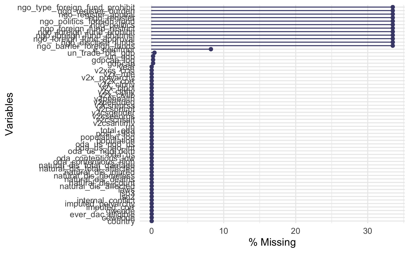
There are only three countries now that have any missing data:
Kosovo is missing pre-existence infant mortality, which is fine becuase it didn’t exist yet.
Russia is missing GDP, GDP per capita, and percent of GDP from trade from 1980–1989. There’s no easy way around this. V-Dem has GDP per capita data from the long-running Maddison Project Database, and it includes 1980s Soviet Russia, but the values aren’t really comparable to the stuff we calculated using UN GDP data. At first glance it seems that this is a difference in real years, since the Maddison Project uses 2011 dollars and the UN uses 2015 dollars, and there’s not an easy way to shift the Maddison Project’s values up to 2015 (i.e. there’s no deflator). But even if they were in the same dollar-years, the values from the Maddison Project seem really really low compared to what we made with the UN GDP data, so they don’t seem to be comparable.
Czechoslovakia is missing percent of GDP from trade from 1980–1989. This is because it is missing imports data in the UN GDP data. It has exports data and overall GDP data, but for whatever reason, imports are missing. Boo.
country_aid_complete %>%
  select(gwcode, country, year, un_trade_pct_gdp, un_gdp, gdpcap, gdpcap_log) %>%
  filter(is.na(un_trade_pct_gdp))
## gwcode country year un_trade_pct_gdp un_gdp gdpcap gdpcap_log
## 1 316 Czechia 1980 NA 183919110258 17771.54 9.785353
## 2 316 Czechia 1981 NA 183743647861 17726.42 9.782812
## 3 316 Czechia 1982 NA 183984035455 17750.06 9.784144
## 4 316 Czechia 1983 NA 188240745011 18180.31 9.808094
## 5 316 Czechia 1984 NA 194289061254 18788.90 9.841022
## 6 316 Czechia 1985 NA 199875093661 19346.85 9.870285
## 7 316 Czechia 1986 NA 205065586592 19856.67 9.896295
## 8 316 Czechia 1987 NA 209182118795 20254.92 9.916153
## 9 316 Czechia 1988 NA 214531745219 20765.98 9.941071
## 10 316 Czechia 1989 NA 215359391664 20836.11 9.944443
## 11 365 Russia 1980 NA NA NA NA
## 12 365 Russia 1981 NA NA NA NA
## 13 365 Russia 1982 NA NA NA NA
## 14 365 Russia 1983 NA NA NA NA
## 15 365 Russia 1984 NA NA NA NA
## 16 365 Russia 1985 NA NA NA NA
## 17 365 Russia 1986 NA NA NA NA
## 18 365 Russia 1987 NA NA NA NA
## 19 365 Russia 1988 NA NA NA NA
## 20 365 Russia 1989 NA NA NA NASince those issues are all pre-1990, our data is perfect post-1990 in cases with Suparna’s law coverage:
country_aid_complete %>%
  filter(laws) %>%
  gg_miss_var(., show_pct = TRUE)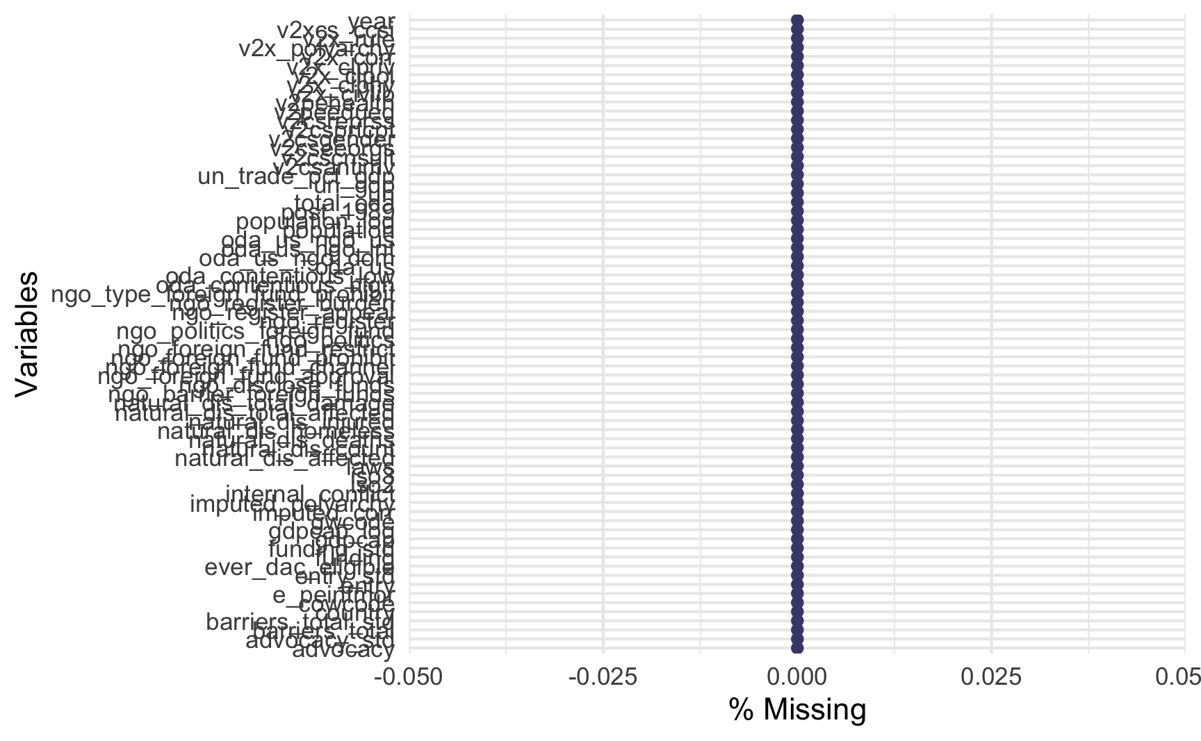
Final data
Now that we know all the data is clean and pretty much nothing is missing, we can do a few final windowed operations that will add missing values (e.g. lagging). We also add an indicator marking if a disaster happened in the past 5 years.
In H3 we hypothesize that more aid will be allocated to international or US-based NGOs than domestic NGOs in response to harsher anti-NGO restrictions. While AidData unfortunately does not categorize aid by channel (i.e. aid given to international vs. US vs. domestic NGOs), USAID does. For this hypothesis, then we only look at aid given by USAID, not the rest of the OECD. As with the proportion of contentious aid, we create similar variables to measure the proportion of aid given to international NGOs, US-based NGOs, and both international and US-based NGOs.
# Determine if any of the values in the last k rows are TRUE
check_last_k <- function(x, k) {
  # This creates a matrix with a column for each lag value (e.g. column 1 = lag
  # 0, column 2 = lag 1, etc.)
  all_lags <- sapply(0:k, FUN = function(k) lag(x, k))

  # Mark TRUE if any of the columns have TRUE in them
  any_true_in_window <- apply(all_lags, MARGIN = 1, FUN = any, na.rm = TRUE)
  return(any_true_in_window)
}

country_aid_final <- country_aid_complete %>%
  # Proportion of contentious aid
  mutate(prop_contentious = oda_contentious_high /
           (oda_contentious_low + oda_contentious_high),
         prop_contentious =
           ifelse(oda_contentious_high == 0 & oda_contentious_low == 0,
                  0, prop_contentious)) %>%
  mutate(prop_contentious_logit = car::logit(prop_contentious, adjust = 0.001)) %>%
  # Proportion of aid to NGOs
  mutate(prop_ngo_int = oda_us_ngo_int / oda_us,
         prop_ngo_us = oda_us_ngo_us / oda_us,
         prop_ngo_dom = oda_us_ngo_dom / oda_us,
         prop_ngo_foreign = (oda_us_ngo_int + oda_us_ngo_us) / oda_us) %>%
  mutate(across(starts_with("prop_ngo"), ~ifelse(is.nan(.), 0, .))) %>%
  mutate(across(starts_with("prop_ngo"), list(logit = ~car::logit(., adjust = 0.001)))) %>%
  mutate(across(c(total_oda, oda_contentious_high, oda_contentious_low, oda_us),
         list(log = ~log1p(.)))) %>%
  # Lag/lead/diff things within countries
  group_by(gwcode) %>%
  # Determine if there was conflict in the past 5 years
  mutate(internal_conflict_past_5 = check_last_k(internal_conflict, 5),
         natural_dis_past_5 = check_last_k(natural_dis_count >= 1, 5)) %>%
  # Indicate changes in laws
  mutate(across(c(advocacy, entry, funding, barriers_total),
                list(new = ~. - lag(.),
                     worse = ~(. - lag(.)) > 0,
                     cat = ~cut(. - lag(.),
                                breaks = c(-Inf, -1, 0, Inf),
                                labels = c("New better law", "No new laws",
                                           "New worse law"),
                                ordered_result = TRUE)))) %>%
  # Lag and lead stuff
  mutate(across(c(barriers_total, advocacy, entry, funding, v2xcs_ccsi,
                  total_oda, total_oda_log, prop_contentious,
                  prop_ngo_dom, prop_ngo_foreign),
                list(lag1 = ~lag(., n = 1)))) %>%
  mutate(across(c(total_oda, total_oda_log, prop_contentious,
                  prop_ngo_dom, prop_ngo_foreign),
                list(lead1 = ~lead(., n = 1)))) %>%
  ungroup()
Save data
Phew. Everything checks out. Save this stuff for use in actual analyses in /data/derived_data/
saveRDS(country_aid_final, here("data", "derived_data", "df_country_aid.rds"))
saveRDS(donor_level_data, here("data", "derived_data", "df_donor.rds"))
saveRDS(donor_level_data_usaid, here("data", "derived_data", "df_donor_usaid.rds"))
saveRDS(autocracies_final, here("data", "derived_data", "df_autocracies.rds"))