H₁: Effect of anti-NGO crackdown on total ODA

library(tidyverse)
library(brms)
library(tidybayes)
library(bayesplot)
library(fixest)
library(broom)
library(broom.mixed)
library(modelsummary)
library(patchwork)
library(tictoc)
library(latex2exp)
library(scales)
library(here)

source(here("lib", "graphics.R"))
source(here("lib", "misc_funs.R"))
color_scheme_set("viridisC")

labs_exp_logged <- function(brks) {TeX(paste0("e^{", as.character(log(brks))), "}")}
labs_exp <- function(brks) {TeX(paste0("e^{", as.character(brks)), "}")}

my_seed <- 1234
set.seed(my_seed)

options(mc.cores = parallel::detectCores(),  # Use all possible cores
        brms.backend = "rstan")

CHAINS <- 4
ITER <- 2000
WARMUP <- 1000
BAYES_SEED <- 1234

# Load data
df_country_aid <- readRDS(here("data", "derived_data", "df_country_aid.rds"))
df_country_aid_laws <- filter(df_country_aid, laws)

Weight models

• Numerator is treatment + non-varying confounders
• Denominator is treatment + lagged outcome + time-varying confounders + non-varying confounders

\[ sw = \prod^t_{t = 1} \frac{\phi(T_{it} | T_{i, t-1}, C_i)}{\phi(T_{it} | T_{i, t-1}, D_{i, t-1}, C_i)} \]

Priors for weight models

We use generic weakly informative priors for our model parameters:

• Intercept: \(\mathcal{N} (0, 10)\)
• Coefficients: \(\mathcal{N} (0, 2.5)\)
• Sigma: \(\operatorname{Cauchy} (0, 1)\)

pri_int <- ggplot() +
  stat_function(fun = dnorm, args = list(mean = 0, sd = 10),
                geom = "area", fill = "grey80", color = "black") +
  labs(x = TeX("\\textbf{Intercept (β_0)}")) +
  annotate(geom = "label", x = 0, y = 0.01, label = "N(0, 10)", size = pts(9)) +
  xlim(-40, 40) +
  theme_donors(prior = TRUE)

pri_coef <- ggplot() +
  stat_function(fun = dnorm, args = list(mean = 0, sd = 2.5),
                geom = "area", fill = "grey80", color = "black") +
  labs(x = TeX("\\textbf{Coefficients (β_x)}")) +
  annotate(geom = "label", x = 0, y = 0.04, label = "N(0, 3)", size = pts(9)) +
  xlim(-10, 10) +
  theme_donors(prior = TRUE)

pri_sigma <- ggplot() +
  stat_function(fun = dcauchy, args = list(location = 0, scale = 1),
                geom = "area", fill = "grey80", color = "black") +
  labs(x = "σ") +
  annotate(geom = "label", x = 5, y = 0.08, label = "Cauchy(0, 1)", size = pts(9)) +
  xlim(0, 10) +
  theme_donors(prior = TRUE)

(pri_int + pri_coef + pri_sigma)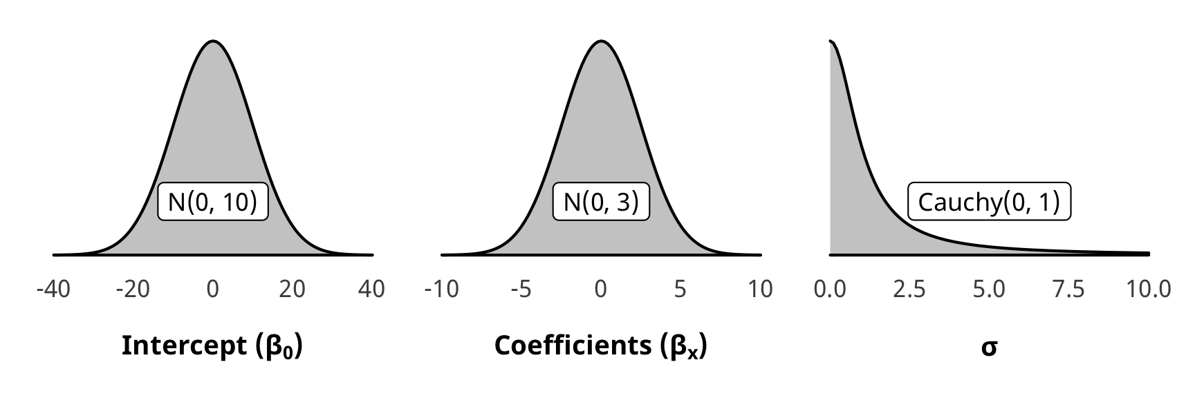

Run weight models

# Numerator ---------------------------------------------------------------
# Formulas
# Treatment ~ lag treatment + non-varying confounders
formula_h1_num_total <- bf(barriers_total ~ barriers_total_lag1 + (1 | gwcode))
formula_h1_num_advocacy <- bf(advocacy ~ advocacy_lag1 + (1 | gwcode))
formula_h1_num_entry <- bf(entry ~ entry_lag1 + (1 | gwcode))
formula_h1_num_funding <- bf(funding ~ funding_lag1 + (1 | gwcode))

# Priors
prior_num <- c(set_prior("normal(0, 10)", class = "Intercept"),
               set_prior("normal(0, 2.5)", class = "b"),
               set_prior("cauchy(0, 1)", class = "sd"))


# Denominator -------------------------------------------------------------
# Formulas
# Treatment ~ lag treatment + lag outcome + varying confounders + non-varying confounders
formula_h1_denom_total <- 
  bf(barriers_total ~ barriers_total_lag1 + total_oda_log_lag1 +
       # Human rights and politics
       v2x_polyarchy + v2x_corr + v2x_rule + v2x_civlib + v2x_clphy + v2x_clpriv +
       # Economics and development
       gdpcap_log + un_trade_pct_gdp + v2peedueq + v2pehealth + e_peinfmor +
       # Conflict and disasters
       internal_conflict_past_5 + natural_dis_count +
       (1 | gwcode))

formula_h1_denom_advocacy <- 
  bf(advocacy ~ advocacy_lag1 + total_oda_log_lag1 +
       v2x_polyarchy + v2x_corr + v2x_rule + v2x_civlib + v2x_clphy + v2x_clpriv +
       gdpcap_log + un_trade_pct_gdp + v2peedueq + v2pehealth + e_peinfmor +
       internal_conflict_past_5 + natural_dis_count +
       (1 | gwcode))

formula_h1_denom_entry <- 
  bf(entry ~ entry_lag1 + total_oda_log_lag1 +
       v2x_polyarchy + v2x_corr + v2x_rule + v2x_civlib + v2x_clphy + v2x_clpriv +
       gdpcap_log + un_trade_pct_gdp + v2peedueq + v2pehealth + e_peinfmor +
       internal_conflict_past_5 + natural_dis_count +
       (1 | gwcode))

formula_h1_denom_funding <- 
  bf(funding ~ funding_lag1 + total_oda_log_lag1 +
       v2x_polyarchy + v2x_corr + v2x_rule + v2x_civlib + v2x_clphy + v2x_clpriv +
       gdpcap_log + un_trade_pct_gdp + v2peedueq + v2pehealth + e_peinfmor +
       internal_conflict_past_5 + natural_dis_count +
       (1 | gwcode))

# Priors
prior_denom <- c(set_prior("normal(0, 10)", class = "Intercept"),
                 set_prior("normal(0, 2.5)", class = "b"),
                 set_prior("normal(0, 2.5)", class = "sd"))


# Run weighting models ----------------------------------------------------
# All models get run inside a tibble using map() magic
all_models_h1 <- tribble(
  ~model_name, ~formula_num, ~formula_denom,
  "h1_total", formula_h1_num_total, formula_h1_denom_total,
  "h1_advocacy", formula_h1_num_advocacy, formula_h1_denom_advocacy,
  "h1_entry", formula_h1_num_entry, formula_h1_denom_entry,
  "h1_funding", formula_h1_num_funding, formula_h1_denom_funding
)

# Fit models
tic()
fit_h1_all_models <- all_models_h1 %>%
  mutate(fit_num = map2(formula_num, model_name, ~brm(
    .x,
    data = df_country_aid_laws,
    prior = prior_num,
    iter = ITER, chains = CHAINS, warmup = WARMUP, seed = BAYES_SEED,
    control = list(adapt_delta = 0.99),
    file = here("analysis", "model_cache", paste0(.y, "_num.rds"))
  ))) %>%
  mutate(fit_denom = map2(formula_denom, model_name, ~brm(
    .x,
    data = df_country_aid_laws,
    prior = prior_denom,
    iter = ITER, chains = CHAINS, warmup = WARMUP, seed = BAYES_SEED,
    control = list(adapt_delta = 0.9),
    file = here("analysis", "model_cache", paste0(.y, "_denom.rds"))
  ))) 
fit_h1_all_models
toc()

Check weight models

We check a few of the numerator and denominator models for convergence and mixing and fit.

Numerator

check_total_num <- fit_h1_all_models %>% 
  filter(model_name == "h1_total") %>% pull(fit_num) %>% first()

pp_check(check_total_num, type = "dens_overlay", nsamples = 10) +
  theme_donors()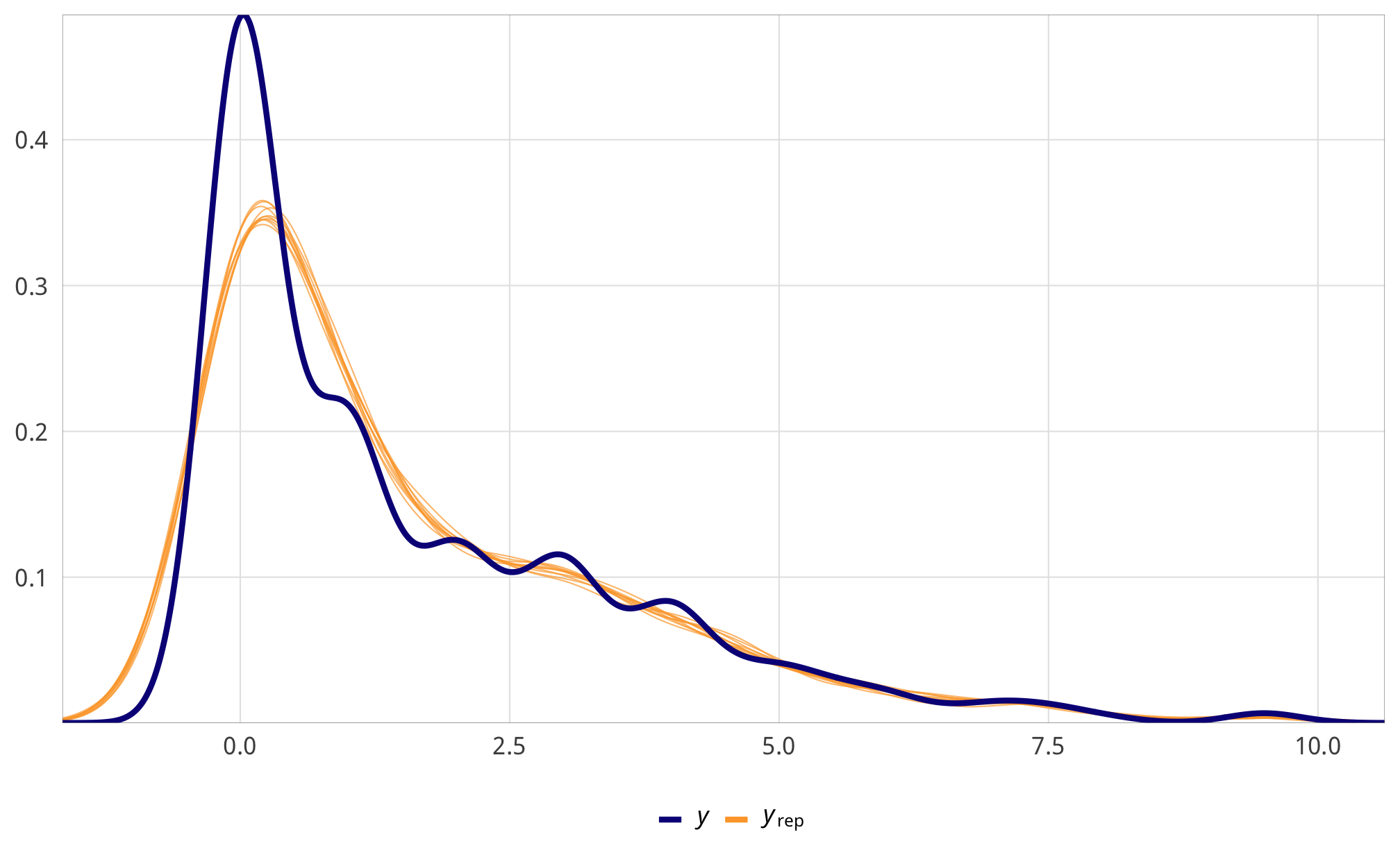

check_total_num %>% 
  posterior_samples(add_chain = TRUE) %>% 
  select(-starts_with("r_gwcode"), -starts_with("z_"), -lp__, -iter) %>% 
  mcmc_trace() +
  theme_donors() +
  theme(legend.position = c(0.72, 0.38))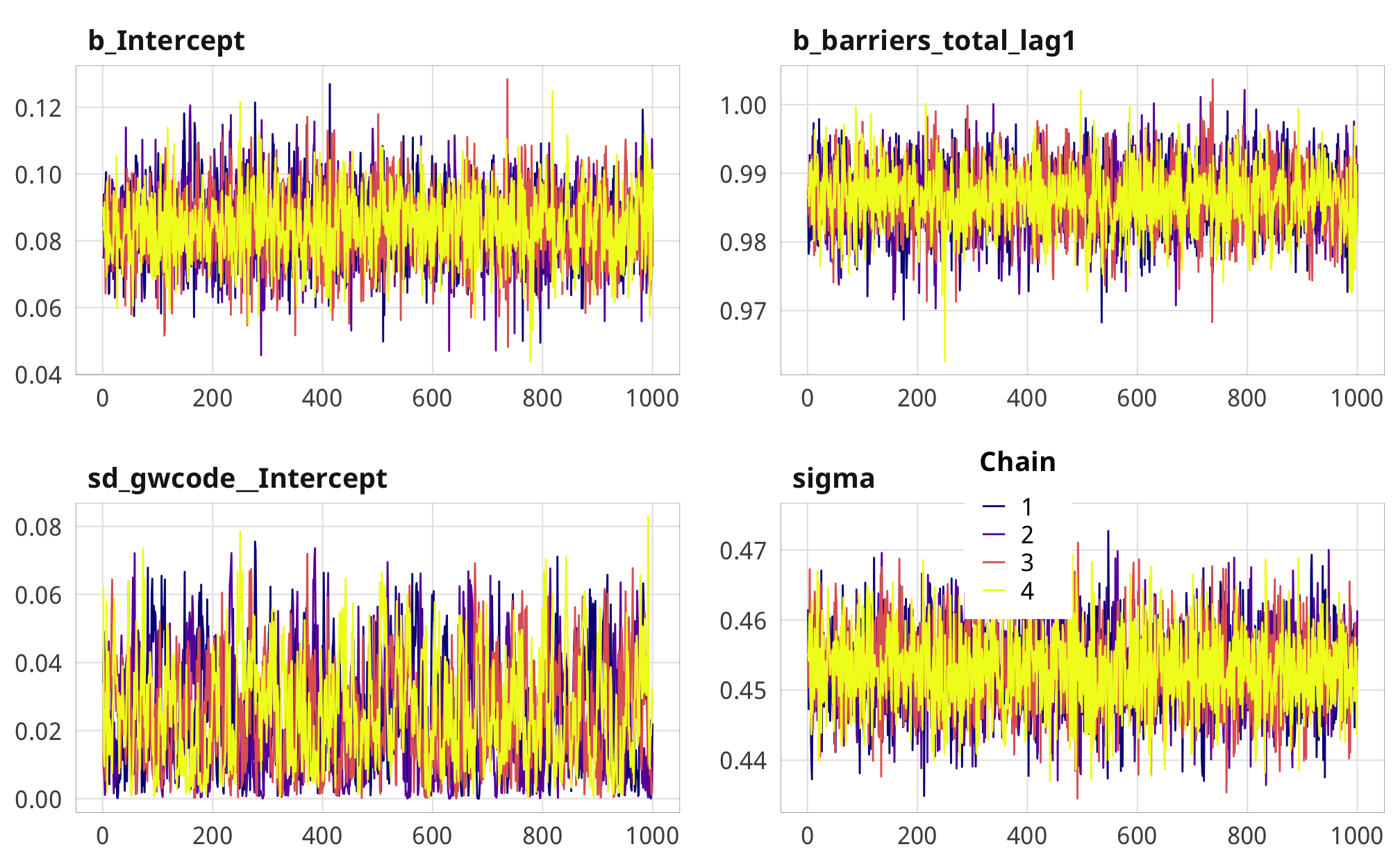

Denominator

check_total_denom <- fit_h1_all_models %>% 
  filter(model_name == "h1_total") %>% pull(fit_denom) %>% first()

pp_check(check_total_denom, type = "dens_overlay", nsamples = 10) +
  theme_donors()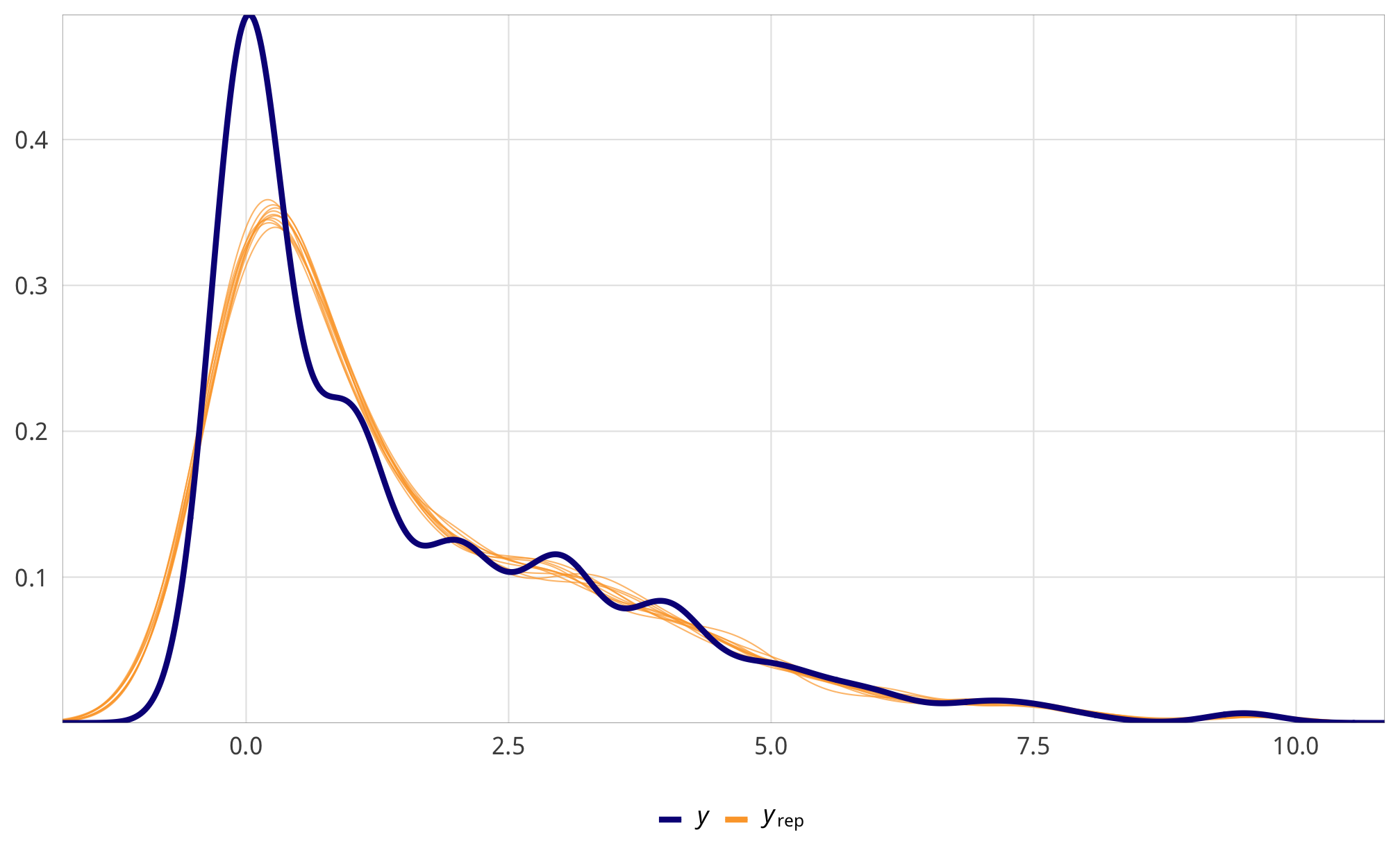

check_total_denom %>% 
  posterior_samples(add_chain = TRUE) %>% 
  select(-starts_with("r_gwcode"), -starts_with("z_"), -lp__, -iter) %>% 
  mcmc_trace() +
  theme_donors() +
  theme(legend.position = "right")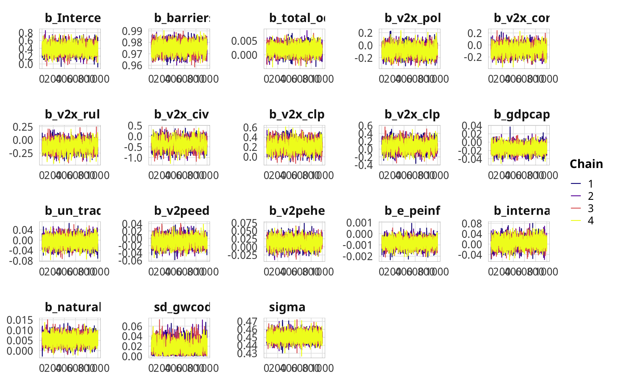

Build weights

# This is the tidybayes way to calculate predictions and residuals but holy crap
# it's sloooow and memory intensive, so we use predict.brmsfit() instead
#
# predicted_num <- df_country_aid_laws %>%
#   add_predicted_draws(fit_num) %>%
#   mutate(.residual = barriers_total - .prediction)
# 
# predicted_num_per_row <- predicted_num %>%
#   group_by(.row) %>%
#   mean_hdi(.prediction, .residual)

tic()
fit_h1_preds <- fit_h1_all_models %>%
  mutate(pred_num = map(fit_num, ~predict(.x, newdata = df_country_aid_laws, allow_new_levels = TRUE)),
         resid_num = map(fit_num, ~residuals(.x, newdata = df_country_aid_laws, allow_new_levels = TRUE)),
         pred_denom = map(fit_denom, ~predict(.x, newdata = df_country_aid_laws, allow_new_levels = TRUE)),
         resid_denom = map(fit_denom, ~residuals(.x, newdata = df_country_aid_laws, allow_new_levels = TRUE)))
toc()

## 101.157 sec elapsed

fit_h1_ipw <- fit_h1_preds %>%
  mutate(num_actual = pmap(list(form = formula_num, pred = pred_num, resid = resid_num), 
                           calc_prob_dist),
         denom_actual = pmap(list(form = formula_denom, pred = pred_denom, resid = resid_denom), 
                          calc_prob_dist)) %>% 
  mutate(df_with_weights = map2(num_actual, denom_actual, ~{
    df_country_aid_laws %>% 
      mutate(weights_sans_time = .x / .y) %>% 
      group_by(gwcode) %>% 
      mutate(ipw = cumprod_na(weights_sans_time)) %>% 
      ungroup()
  }))
fit_h1_ipw

## # A tibble: 4 x 12
##   model_name formula_num formula_denom fit_num fit_denom pred_num resid_num pred_denom
##   <chr>      <list>      <list>        <list>  <list>    <list>   <list>    <list>    
## 1 h1_total   <brmsfrml>  <brmsfrml>    <brmsf… <brmsfit> <dbl[,4… <dbl[,4]… <dbl[,4] …
## 2 h1_advoca… <brmsfrml>  <brmsfrml>    <brmsf… <brmsfit> <dbl[,4… <dbl[,4]… <dbl[,4] …
## 3 h1_entry   <brmsfrml>  <brmsfrml>    <brmsf… <brmsfit> <dbl[,4… <dbl[,4]… <dbl[,4] …
## 4 h1_funding <brmsfrml>  <brmsfrml>    <brmsf… <brmsfit> <dbl[,4… <dbl[,4]… <dbl[,4] …
## # … with 4 more variables: resid_denom <list>, num_actual <list>, denom_actual <list>,
## #   df_with_weights <list>

Outcome models

Modeling choice

Total aid has a ton of zeroes, but the zeroes are really far away from the distribution of the actual data, so rather than be zero-inflated, this represents a hurdle process. Something determines whether a country/year receives any aid, and then something else determines how much.

If we don’t take this hurdling process into account in the model, our ATE will be wrong. We don’t really care about the exact hurdling process—we care most about the ATE of laws/restrictions on aid—but we still need to deal with the hurdle.

aid_hist_original <- ggplot(df_country_aid_laws, aes(x = total_oda)) +
  geom_histogram(binwidth = 2e9, color = "white", boundary = 0) +
  scale_x_continuous(labels = scales::dollar) +
  labs(x = "Total ODA", y = "Count", 
       title = "ODA") +
  theme_donors()

aid_hist_logged <- ggplot(df_country_aid_laws, aes(x = total_oda_log)) +
  geom_histogram(binwidth = 1, color = "white", boundary = 0) +
  labs(x = "Total ODA (logged)", y = "Count", 
       title = "Logged ODA") +
  theme_donors()

aid_hist_original + aid_hist_logged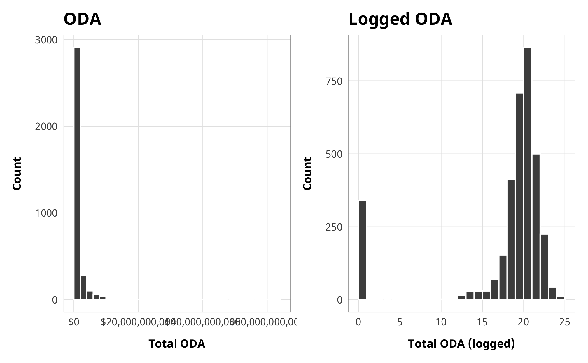

So we fit a hurdled lognormal model, which uses a logit model to predict 0/not 0, then uses a lognormal distribution to model the rest of the data. The hurdle_lognormal() family is already built in to brms which is nice. It’s possible to create custom families like hurdle_gaussian(), but this is super hard to do. I have an implementation partially completed here, but I can’t get it to actually create posterior predictions. Ugh.

Fortunately the lognormal family works well here, since foreign aid follows an exponential distribution and we were using log aid originally. Now we don’t have to use log aid and can model the hurdle process at the same time without relying on my own rickety hurdle_gaussian() function.

For comparison, here’s a regular gaussian model using log ODA and sans hurdling.

# Extract the data with weights for the barriers_total model
aid_data_example_wts <- fit_h1_ipw %>% 
  filter(model_name == "h1_total") %>% 
  pull(df_with_weights) %>% first()

example_normal_fit <- brm(
  bf(total_oda_log_lead1 | weights(ipw) ~ barriers_total + (1 | gwcode)),
  data = aid_data_example_wts,
  family = gaussian(), 
  iter = ITER, chains = CHAINS, warmup = WARMUP, seed = BAYES_SEED,
  file = here("analysis", "model_cache", paste0("h1_example_normal.rds"))
)

example_hu_fit <- brm(
  bf(total_oda_lead1 | weights(ipw) ~ barriers_total + (1 | gwcode), 
     hu ~ 1),
  data = aid_data_example_wts,
  # Have to use rstan because cmdstanr weirdly uses negative inits
  family = hurdle_lognormal(), backend = "rstan",
  iter = ITER * 2, chains = CHAINS, warmup = WARMUP, seed = BAYES_SEED,
  file = here("analysis", "model_cache", paste0("h1_example_hurdle.rds"))
)

Even though we just used an intercept-only model for the hurdle process, incorporating it into the overall model gives us a much better fit. Look at these posterior predictive checks:

pp_check(example_normal_fit, type = "dens_overlay", nsamples = 10) + 
  coord_cartesian(xlim = c(0, 30)) +
  scale_x_continuous(labels = labs_exp) +
  labs(title = "log(y) ~ x, gaussian family, no hurdling") +
  theme_donors()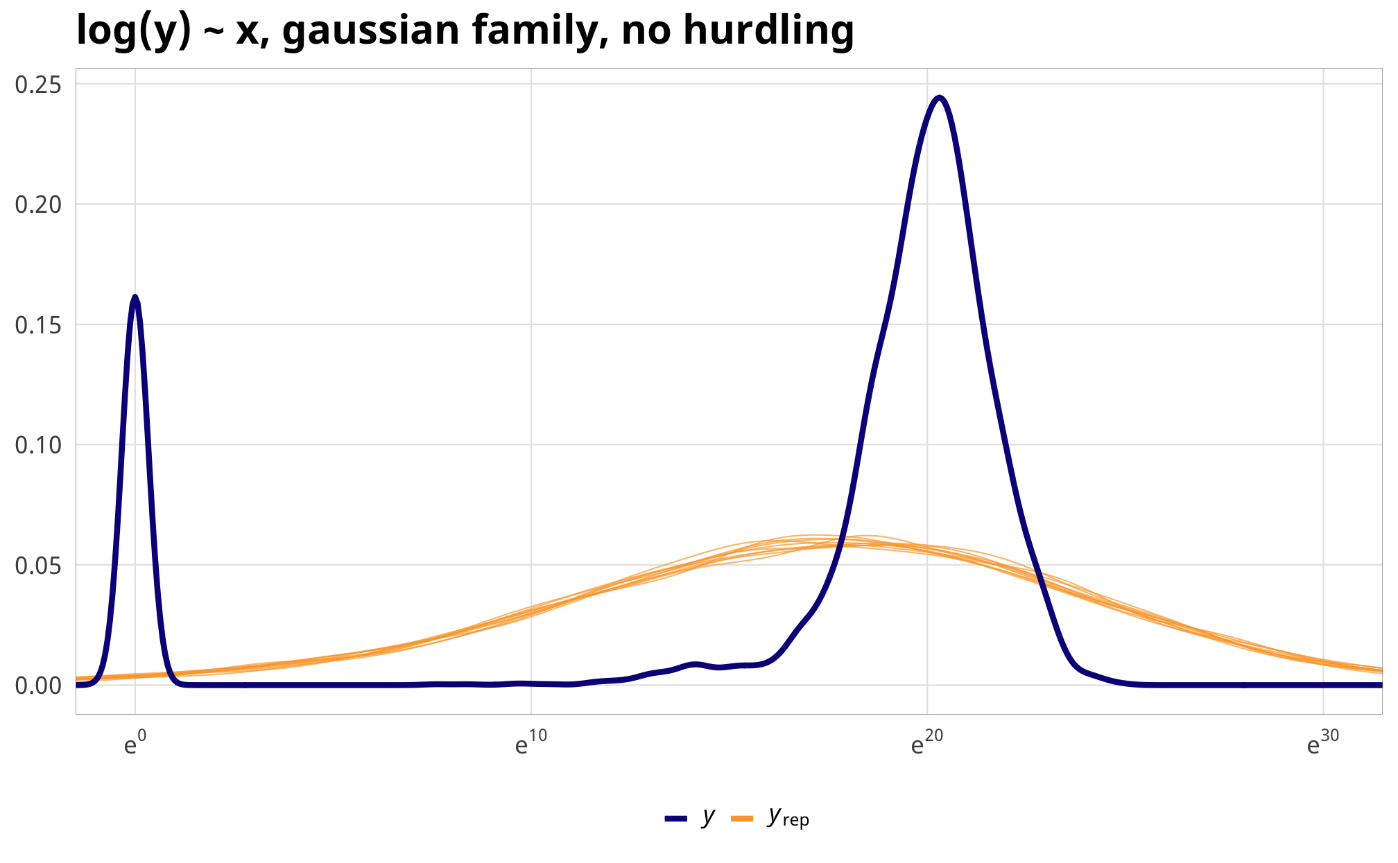

pp_check(example_hu_fit, type = "dens_overlay", nsamples = 10) + 
  scale_x_continuous(trans = "log1p", breaks = exp(seq(0, 30, 5)),
                     labels = labs_exp_logged) +
  labs(title = "y ~ x, lognormal family, hurdle: hu ~ 1") +
  theme_donors()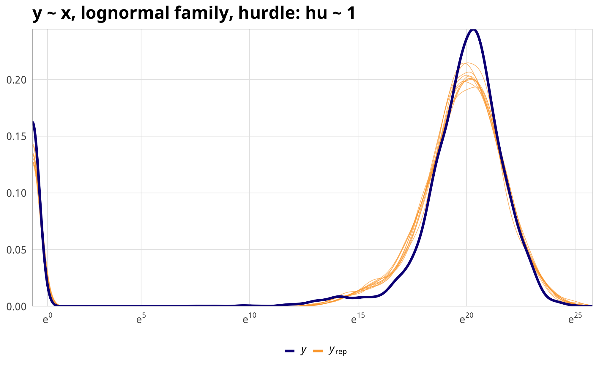

Importantly, the coefficients switch directions!

example_normal_fit %>% 
  gather_draws(b_barriers_total) %>%
  mutate(.variable = dplyr::recode(.variable, 
                                   b_barriers_total = "Additional law, t")) %>% 
  ggplot(aes(y = fct_rev(.variable), x = .value, fill = fct_rev(.variable))) +
  geom_vline(xintercept = 0) +
  stat_halfeye(.width = c(0.8, 0.95), alpha = 0.8) +
  guides(fill = FALSE) +
  scale_x_continuous(labels = scales::percent) +
  scale_fill_manual(values = c("#FF851B", "#FFDC00")) +
  labs(y = NULL, x = "% change in outcome",
       title = "log(y) ~ x, gaussian family, no hurdling") +
  theme_donors()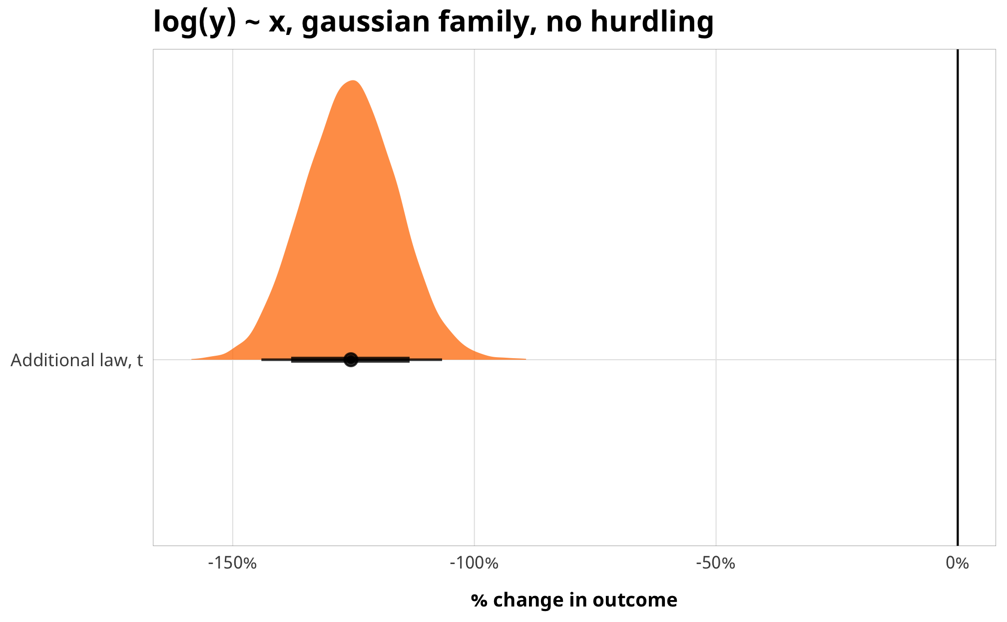

example_hu_fit %>% 
  gather_draws(b_barriers_total) %>%
  mutate(.value = exp(.value) - 1) %>%
  mutate(.variable = dplyr::recode(.variable, 
                                   b_barriers_total = "Additional law, t - 1")) %>% 
  ggplot(aes(y = fct_rev(.variable), x = .value, fill = fct_rev(.variable))) +
  geom_vline(xintercept = 0) +
  stat_halfeye(.width = c(0.8, 0.95), alpha = 0.8) +
  guides(fill = FALSE) +
  scale_x_continuous(labels = scales::percent) +
  scale_fill_manual(values = c("#FF851B", "#FFDC00")) +
  labs(y = NULL, x = "% change in outcome",
       title = "y ~ x, lognormal family; hurdle: hu ~ 1") +
  theme_donors()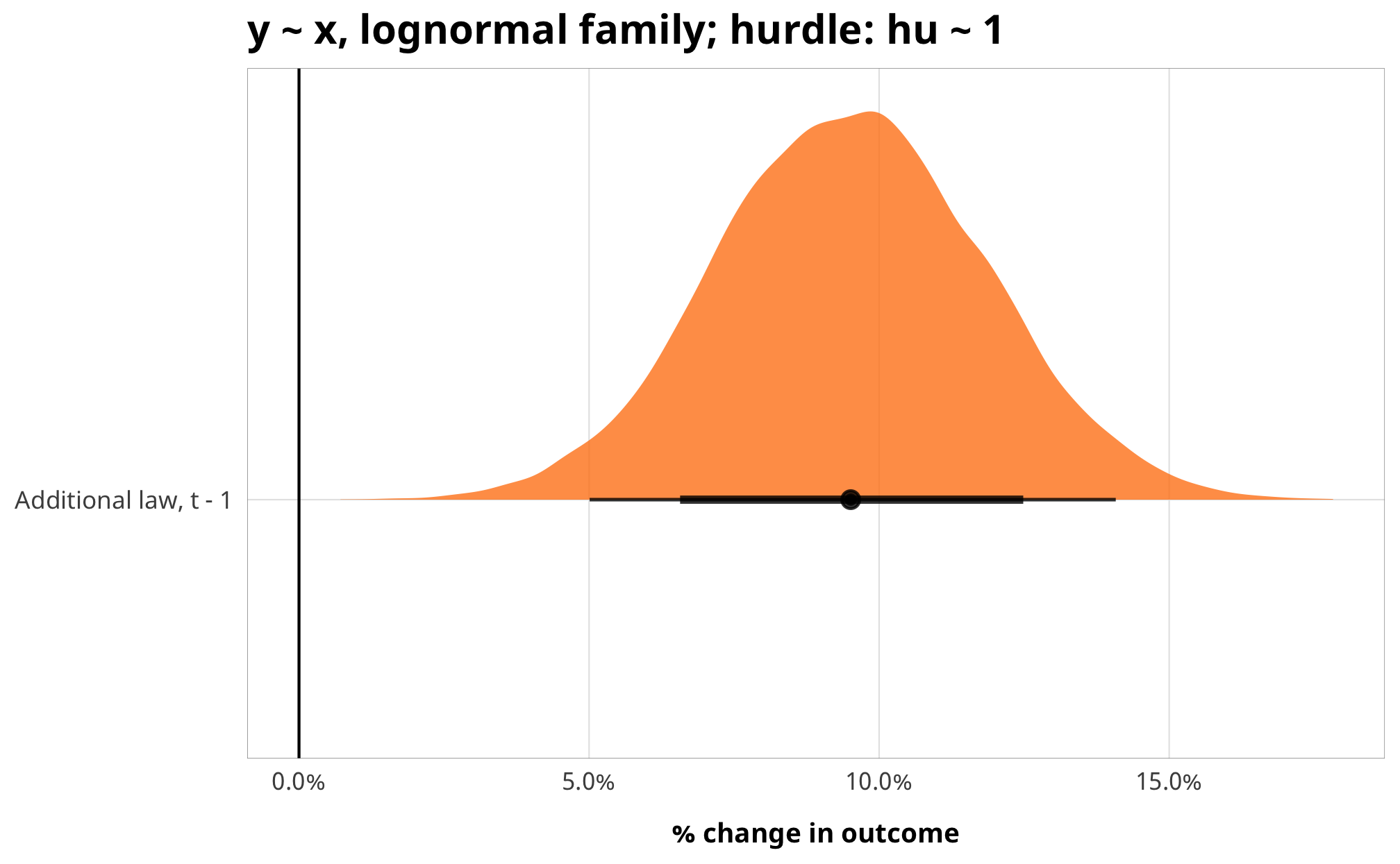

We thus use a lognormal family when modeling the outcome. Because we’re limiting ourselves to just observations that receive aid, our ATE theoretically only shows the effect of treatment on actually having the outcome occur. We’re not trying to model the effect of treatment on the 0/1 logit process for receiving aid in the first place.

Interpreting lognormal models

Because the outcome is pre-logged, we have to interpret these results a little differently from standard OLS, but it’s not too bad, considering that a standard approach to exponential data like aid is to model the logged outcome. When the y is logged, coefficients represent percent changes in y. Models using the lognormal family follow the same principle.

tidy(example_hu_fit) %>%
  mutate(estimate_exp = exp(estimate)) %>% 
  filter(term == "barriers_total") %>% 
  select(term, estimate, estimate_exp)

## # A tibble: 1 x 3
##   term           estimate estimate_exp
##   <chr>             <dbl>        <dbl>
## 1 barriers_total   0.0906         1.09

In the lognormal model, the exponentiated coefficients represent percent changes for each unit increase in X. For instance, \(e^\beta_1\) here is 1.09488 Like exponentiated logistic regression coefficients, everything here is centered around 1, meaning that there’s a 9.49% increase in aid for every legal barrier added. This can be also be seen as a multiplier effect. If aid is $50 million, it changes to $54,744,184 (50,000,000 × 1.09488).

When using brms::fitted() on the model object, brms shows data on the original scale, but to see the intuition behind the percent change, we can calculate the percent change manually. Magically, they’re all around 0.097.

example_hu_fitted_values <- fitted(
  example_hu_fit, 
  newdata = data.frame(barriers_total = seq(0, 8, 1)), 
  re_formula = NA,
  robust = TRUE
)

example_hu_fitted_values %>% 
  as.data.frame() %>% 
  mutate(pct_change = (Estimate - lag(Estimate)) / lag(Estimate))

##     Estimate Est.Error      Q2.5      Q97.5 pct_change
## 1  551061422  73995903 423779255  716564588         NA
## 2  602738400  78980958 467126166  778530995 0.09377716
## 3  660078262  86582957 511314432  854613970 0.09513225
## 4  722358081  96356479 555703369  940877605 0.09435217
## 5  792042599 111060579 601787822 1045672373 0.09646811
## 6  867880647 130321945 647577188 1168121690 0.09574996
## 7  951517880 155182324 693186719 1304630056 0.09636951
## 8 1042581150 182769751 738857268 1465192715 0.09570316
## 9 1141398163 217284639 785081899 1648918248 0.09478112

Interpreting this coefficient gets a little trickier because we used a multilevel model with population and group effects. This \(\beta_1\) here is the average effect for a median cluster at each level of X. See this incredible resource for a ton more details about different ways of piecing together population- and group-level effects in a lognormal model.

I’ve never seen any paper anywhere use hurdled outcome models with MSMs, but I think it legally works here.

Priors for outcome models

There are a ton of moving parts in these outcome models. Here’s the full specification for the models and all priors:

\[ \begin{aligned} \text{Aid}_{i,t} | u_i, \text{Law}_{i, t-1} &\sim \operatorname{LogNormal} (Z_{i, t}, \text{Aid}^\star_{i, t}) & \text{[likelihood]} \\ \operatorname{logit} (Z_{i, t}) &\sim \alpha_Z & \text{[intercept-only logit if } \text{Aid}_{i, t} = 0 \text{]} \\ \log (\text{Aid}^\star_{i, t}) &\sim \mathcal{N} (\beta_0 + \beta_1 \text{Law}_{i, t-1}, \sigma^2_\epsilon, u_i) \times \text{IPW}_{i, t-1} & \text{[if } \text{Aid}_{i, t} > 0 \text{]}\\ u_i &\sim \mathcal{N} (0, \sigma^2_u) & \text{[country-specific intercepts]} \\ \ \\ \alpha_Z &\sim \operatorname{Logistic}(-2, 0.6) & \text{[prior proportion of rows where Aid = 0]} \\ \beta_0 &\sim \mathcal{N} (0, 15) & \text{[prior population intercept]} \\ \beta_1 &\sim \mathcal{N} (0, 3) & \text{[prior population effects]} \\ \sigma^2_e, \sigma^2_u &\sim \operatorname{Cauchy}(0, 1) & \text{[prior sd for population and country]} \\ \ \\ \text{IPW}_{i, t-1} &= \prod^t_{t = 1} \frac{\phi(T_{it} | T_{i, t-1}, C_i)}{\phi(T_{it} | T_{i, t-1}, D_{i, t-1}, C_i)} & \text{[stabilized weights]} \end{aligned} \]

Here’s what those look like:

z_p <- ggplot() +
  stat_function(fun = dlogis, args = list(location = -2, scale = 0.6),
                geom = "area", fill = "grey80", color = "black") +
  labs(x = TeX("\\textbf{Proportion where Aid = 0 (α_Z)}")) +
  annotate(geom = "label", x = -2, y = 0.07, label = "Logistic(-2, 0.6)", size = pts(9)) +
  xlim(-8, 3) +
  theme_donors(prior = TRUE)

b0_p <- ggplot() +
  stat_function(fun = dnorm, args = list(mean = 0, sd = 15),
                geom = "area", fill = "grey80", color = "black") +
  labs(x = TeX("\\textbf{Population intercept (β_0)}")) +
  annotate(geom = "label", x = 0, y = 0.0042, label = "N(0, 15)", size = pts(9)) +
  xlim(-50, 50) +
  theme_donors(prior = TRUE)

b1_p <- ggplot() +
  stat_function(fun = dnorm, args = list(mean = 0, sd = 3),
                geom = "area", fill = "grey80", color = "black") +
  labs(x = TeX("\\textbf{Population effects (β_1)}")) +
  annotate(geom = "label", x = 0, y = 0.02, label = "N(0, 3)", size = pts(9)) +
  xlim(-10, 10) +
  theme_donors(prior = TRUE)

sigma_p <- ggplot() +
  stat_function(fun = dcauchy, args = list(location = 0, scale = 1),
                geom = "area", fill = "grey80", color = "black") +
  labs(x = TeX("\\textbf{Population and country SD (σ_e, σ_u)}")) +
  annotate(geom = "label", x = 5, y = 0.04, label = "Cauchy(0, 1)", size = pts(9)) +
  xlim(0, 10) +
  theme_donors(prior = TRUE)

(z_p + b0_p) / (b1_p | sigma_p)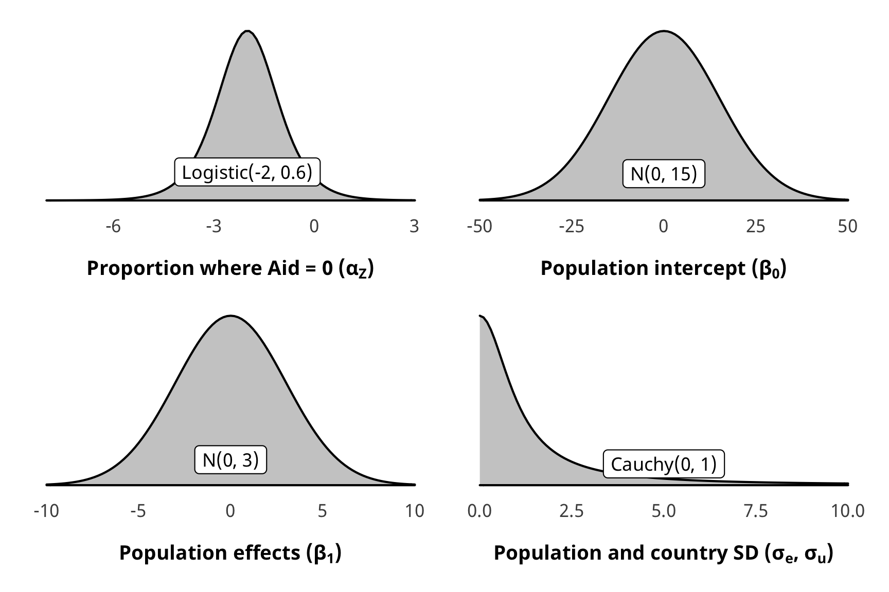

The prior for the hurdle model is a little weird. For whatever reason, brms::get_prior() says that the prior for the hu parameter is beta(0, 1), but in practice, if you run brms::prior_summary() it shows that it actually uses a default of logistic(0, 1), and Stan yells at you if you use a beta prior. Ideally, we want a beta(2, 11) prior, but we can’t specify it like that—we have to translate it to a logistic distribution instead. There’s not an easy way to do this, so we used brms::logit_scaled to show the beta distribution on the logit scale, then we played with the location and scale parameters in rlogis() until it looked roughly equivalent.

hu_prior_sim <- tibble(beta = rbeta(10000, 2, 11)) %>% 
  mutate(beta_logit_scale = brms::logit_scaled(beta)) %>% 
  mutate(logit_betaish_prior = rlogis(10000, -2, 0.6)) %>% 
  mutate(prior_probs = plogis(logit_betaish_prior))

hu_prior_plot1 <- ggplot(hu_prior_sim) +
  geom_density(aes(x = beta), fill = "grey80", color = "black") +
  labs(x = "Proportion where Aid = 0",
       subtitle = "Original Beta(2, 11) distribution") +
  coord_cartesian(xlim = c(0, 1)) +
  theme_donors(prior = TRUE)

hu_prior_plot2 <- ggplot(hu_prior_sim) +
  geom_density(aes(x = beta_logit_scale), fill = "grey80", color = "black") +
  labs(x = "Logistic value where Aid = 0",
       subtitle = "Beta(2, 11) scaled with brms::logit_scaled") +
  coord_cartesian(xlim = c(-8, 1)) +
  theme_donors(prior = TRUE)

hu_prior_plot3 <- ggplot(hu_prior_sim) +
  geom_density(aes(x = logit_betaish_prior), fill = "grey80", color = "black") +
  labs(x = "Logistic value where Aid = 0",
       subtitle = "Estimated Logistic(-2, 0.6)") +
  coord_cartesian(xlim = c(-8, 1)) +
  theme_donors(prior = TRUE)

hu_prior_plot4 <- ggplot(hu_prior_sim) +
  geom_density(aes(x = prior_probs), fill = "grey80", color = "black") +
  labs(x = "Proportion where Aid = 0",
       subtitle = "Logistic(-2, 0.6) transformed to probabilities") +
  coord_cartesian(xlim = c(0, 1)) +
  theme_donors(prior = TRUE)

(hu_prior_plot1 + hu_prior_plot2) / (hu_prior_plot3 + hu_prior_plot4)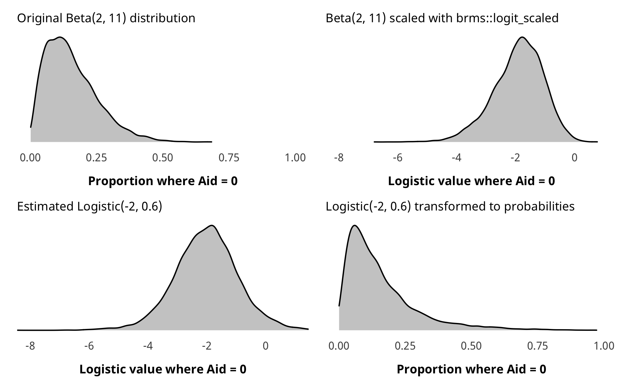

Run outcome models

Phew. With all that out of the way, we can finally run the outcome models.

# Outcome -----------------------------------------------------------------
# Formulas
# Treatment ~ lag treatment + non-varying confounders
formula_h1_out_total <- bf(total_oda_lead1 | weights(ipw) ~ 
                             barriers_total + (1 | gwcode),
                           hu ~ 1)
formula_h1_out_advocacy <- bf(total_oda_lead1 | weights(ipw) ~ 
                             advocacy + (1 | gwcode),
                           hu ~ 1)
formula_h1_out_entry <- bf(total_oda_lead1 | weights(ipw) ~ 
                             entry + (1 | gwcode),
                           hu ~ 1)
formula_h1_out_funding <- bf(total_oda_lead1 | weights(ipw) ~ 
                             funding + (1 | gwcode),
                           hu ~ 1)

# Priors
prior_out <- c(set_prior("normal(0, 20)", class = "Intercept"),
               set_prior("normal(0, 3)", class = "b"),
               set_prior("cauchy(0, 1)", class = "sd"),
               set_prior("logistic(-2, 0.6)", class = "Intercept", dpar = "hu"))

# Run outcome models ------------------------------------------------------
tic()
fit_h1_outcomes <- fit_h1_ipw %>%
  mutate(formula_outcome = 
           list(formula_h1_out_total, formula_h1_out_advocacy, 
                formula_h1_out_entry, formula_h1_out_funding)) %>% 
  mutate(fit_outcome = 
           pmap(list(formula_outcome, df_with_weights, model_name),
                ~brm(
                  ..1,
                  data = ..2,
                  prior = prior_out,
                  family = hurdle_lognormal(),
                  iter = ITER * 2, chains = CHAINS, warmup = WARMUP, seed = BAYES_SEED,
                  # Has to be rstan instead of cmdstanr bc it inexplicably
                  # creates all sorts of nonnegative initialization errors when
                  # using cmdstanr with lognormal() :(
                  backend = "rstan",
                  file = here("analysis", "model_cache", paste0(..3, "_outcome.rds"))
                )))
fit_h1_outcomes
toc()

Check outcome models

check_total_outcome <- fit_h1_outcomes %>% 
  filter(model_name == "h1_total") %>% pull(fit_outcome) %>% first()

pp_check(check_total_outcome, type = "dens_overlay", nsamples = 10) +
  scale_x_continuous(trans = "log1p", breaks = exp(seq(0, 20, 5)),
                     labels = labs_exp_logged) +
  theme_donors()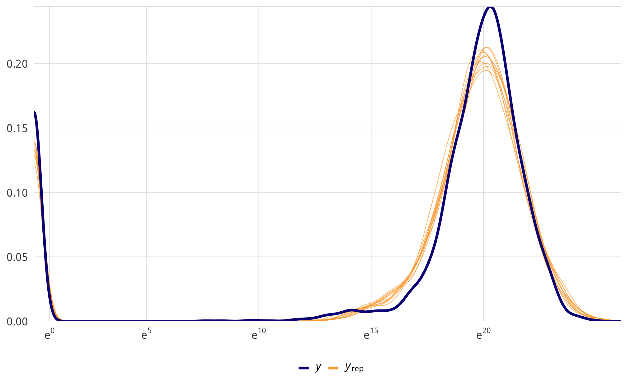

check_total_outcome %>% 
  posterior_samples(add_chain = TRUE) %>% 
  select(-starts_with("r_gwcode"), -starts_with("z_"), -lp__, -iter) %>% 
  mcmc_trace() +
  theme_donors()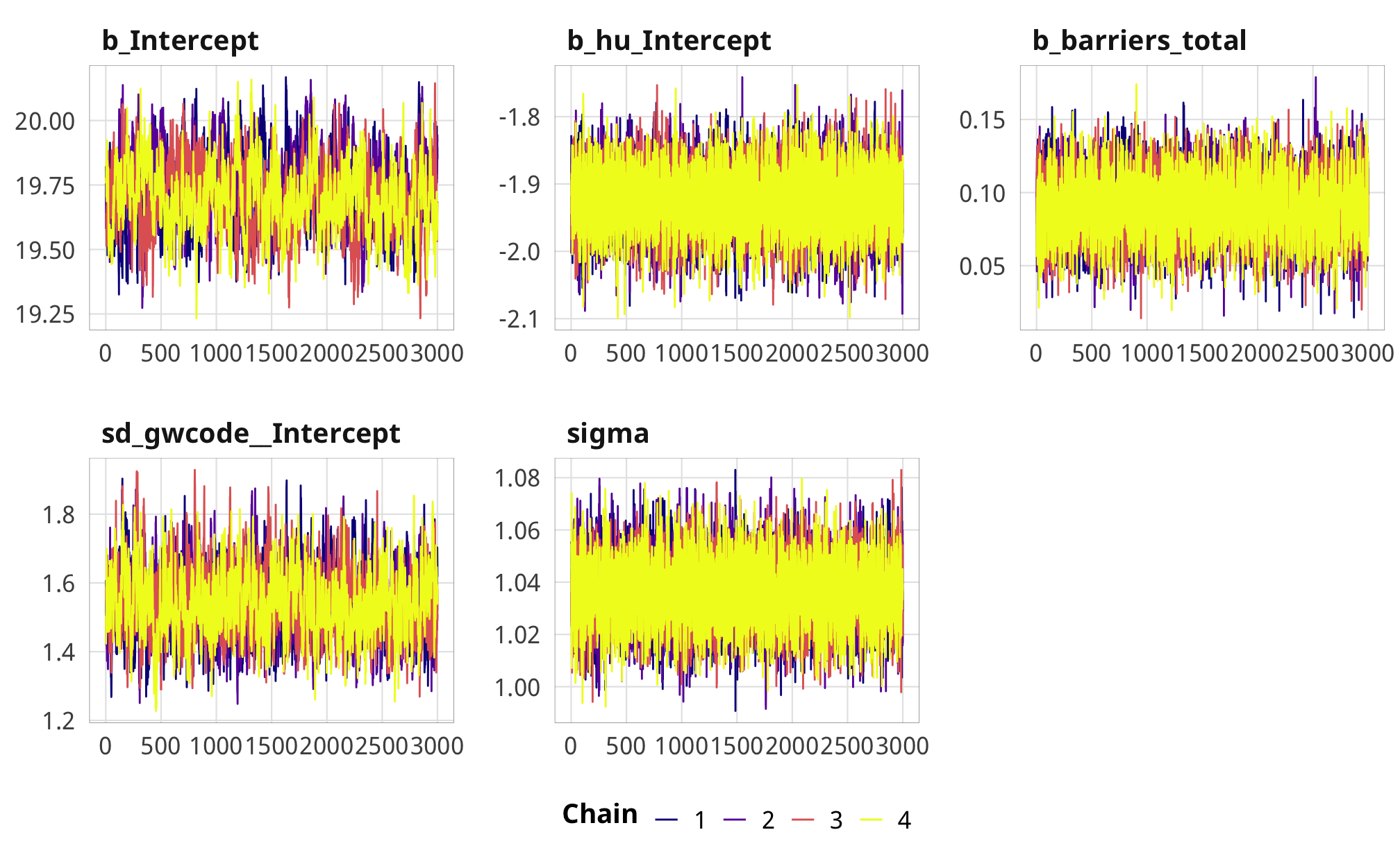

Results

# Plots!
plot_total <- fit_h1_outcomes %>% 
  filter(model_name == "h1_total") %>% 
  pull(fit_outcome) %>% nth(1) %>% 
  gather_draws(b_barriers_total) %>%
  mutate(.value = exp(.value) - 1) %>% 
  mutate(.variable = dplyr::recode(.variable, 
                                   b_barriers_total = "Additional law, t - 1")) %>% 
  ggplot(aes(y = fct_rev(.variable), x = .value, fill = fct_rev(.variable))) +
  geom_vline(xintercept = 0) +
  stat_halfeye(.width = c(0.8, 0.95), alpha = 0.8) +
  guides(fill = FALSE) +
  scale_x_continuous(labels = percent_format(accuracy = 1)) +
  scale_fill_manual(values = c("#FF851B", "#FFDC00")) +
  labs(y = NULL, x = NULL) +
  theme_donors()

plot_advocacy <- fit_h1_outcomes %>% 
  filter(model_name == "h1_advocacy") %>% 
  pull(fit_outcome) %>% nth(1) %>% 
  gather_draws(b_advocacy) %>% 
  mutate(.variable = dplyr::recode(.variable, 
                                   b_advocacy = "Additional advocacy law, t - 1")) %>% 
  mutate(.value = exp(.value) - 1) %>% 
  ggplot(aes(y = fct_rev(.variable), x = .value, fill = fct_rev(.variable))) +
  geom_vline(xintercept = 0) +
  stat_halfeye(.width = c(0.8, 0.95), alpha = 0.8) +
  guides(fill = FALSE) +
  scale_x_continuous(labels = percent_format(accuracy = 1)) +
  scale_fill_manual(values = c("#85144b", "#F012BE")) +
  labs(y = NULL, x = NULL) +
  theme_donors()

plot_entry <- fit_h1_outcomes %>% 
  filter(model_name == "h1_entry") %>% 
  pull(fit_outcome) %>% nth(1) %>% 
  gather_draws(b_entry) %>% 
  mutate(.variable = dplyr::recode(.variable, 
                                   b_entry = "Additional entry law, t - 1")) %>% 
  mutate(.value = exp(.value) - 1) %>% 
  ggplot(aes(y = fct_rev(.variable), x = .value, fill = fct_rev(.variable))) +
  geom_vline(xintercept = 0) +
  stat_halfeye(.width = c(0.8, 0.95), alpha = 0.8) +
  guides(fill = FALSE) +
  scale_x_continuous(labels = percent_format(accuracy = 1)) +
  scale_fill_manual(values = c("#3D9970", "#2ECC40")) +
  labs(y = NULL, x = "% change in ODA") +
  theme_donors()

plot_funding <- fit_h1_outcomes %>% 
  filter(model_name == "h1_funding") %>% 
  pull(fit_outcome) %>% nth(1) %>% 
  gather_draws(b_funding) %>% 
  mutate(.variable = dplyr::recode(.variable, 
                                   b_funding = "Additional funding law, t - 1")) %>% 
  mutate(.value = exp(.value) - 1) %>% 
  ggplot(aes(y = fct_rev(.variable), x = .value, fill = fct_rev(.variable))) +
  geom_vline(xintercept = 0) +
  stat_halfeye(.width = c(0.8, 0.95), alpha = 0.8) +
  guides(fill = FALSE) +
  scale_x_continuous(labels = percent_format(accuracy = 1)) +
  scale_fill_manual(values = c("#001f3f", "#0074D9")) +
  labs(y = NULL, x = "% change in ODA") +
  theme_donors()

(plot_total + plot_advocacy) / (plot_entry + plot_funding)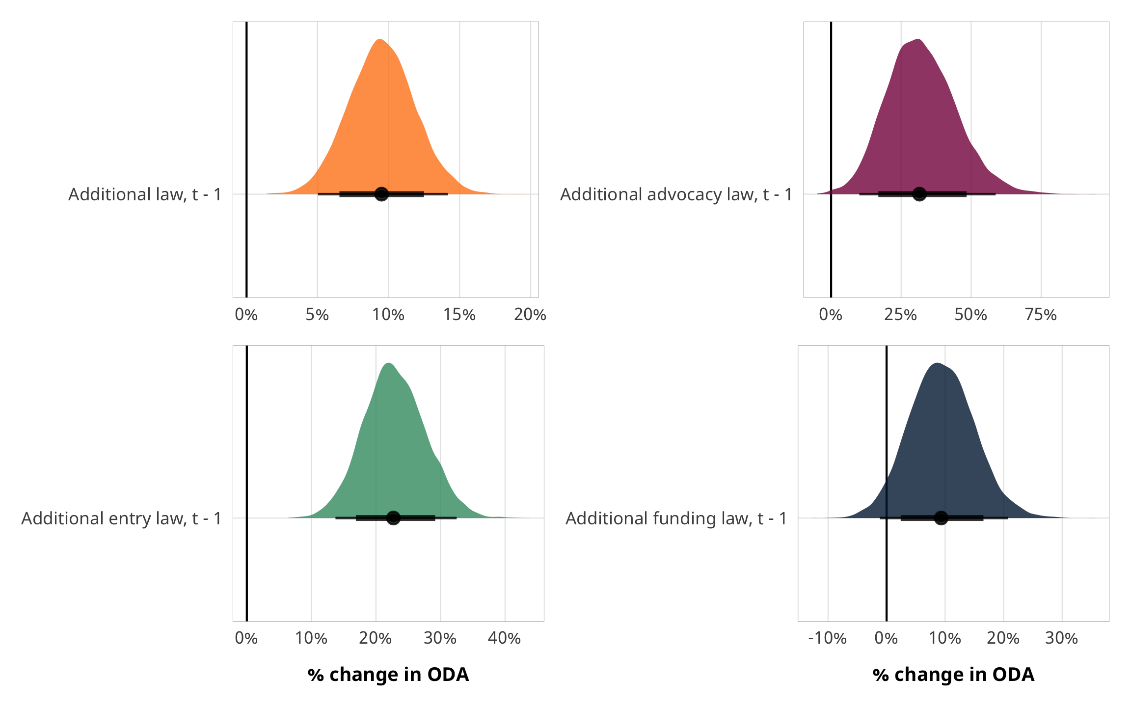

fit_h1_outcomes %>% 
  filter(model_name == "h1_total") %>% 
  pull(fit_outcome) %>% nth(1) %>% 
  conditional_effects()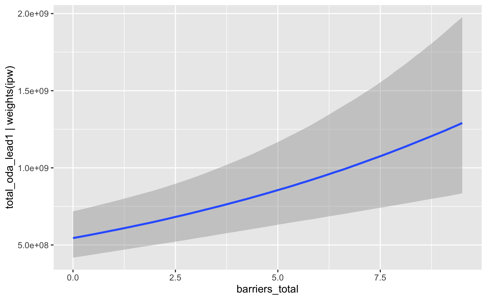

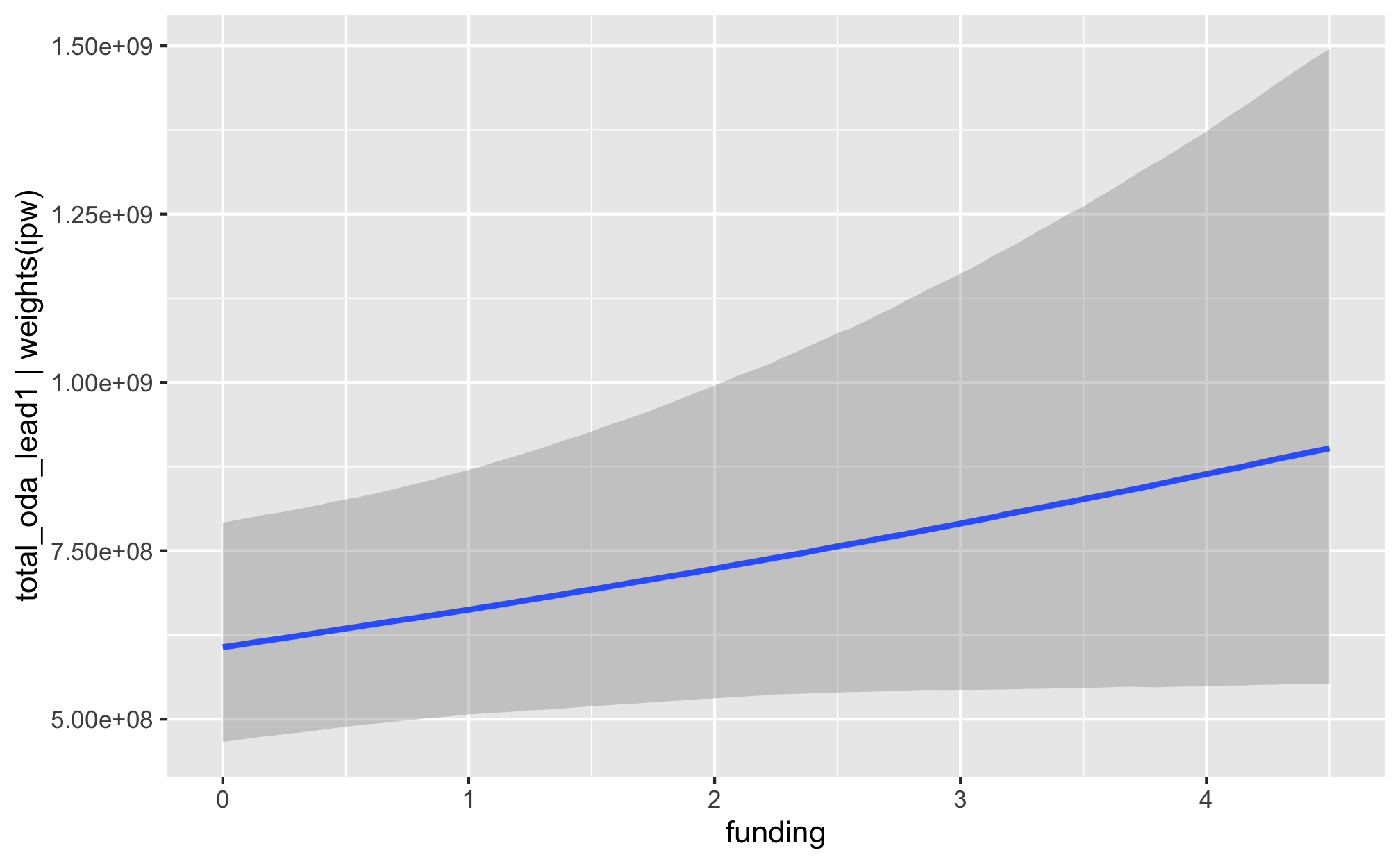
fit_h1_outcomes %>% 
  filter(model_name == "h1_advocacy") %>% 
  pull(fit_outcome) %>% nth(1) %>% 
  conditional_effects()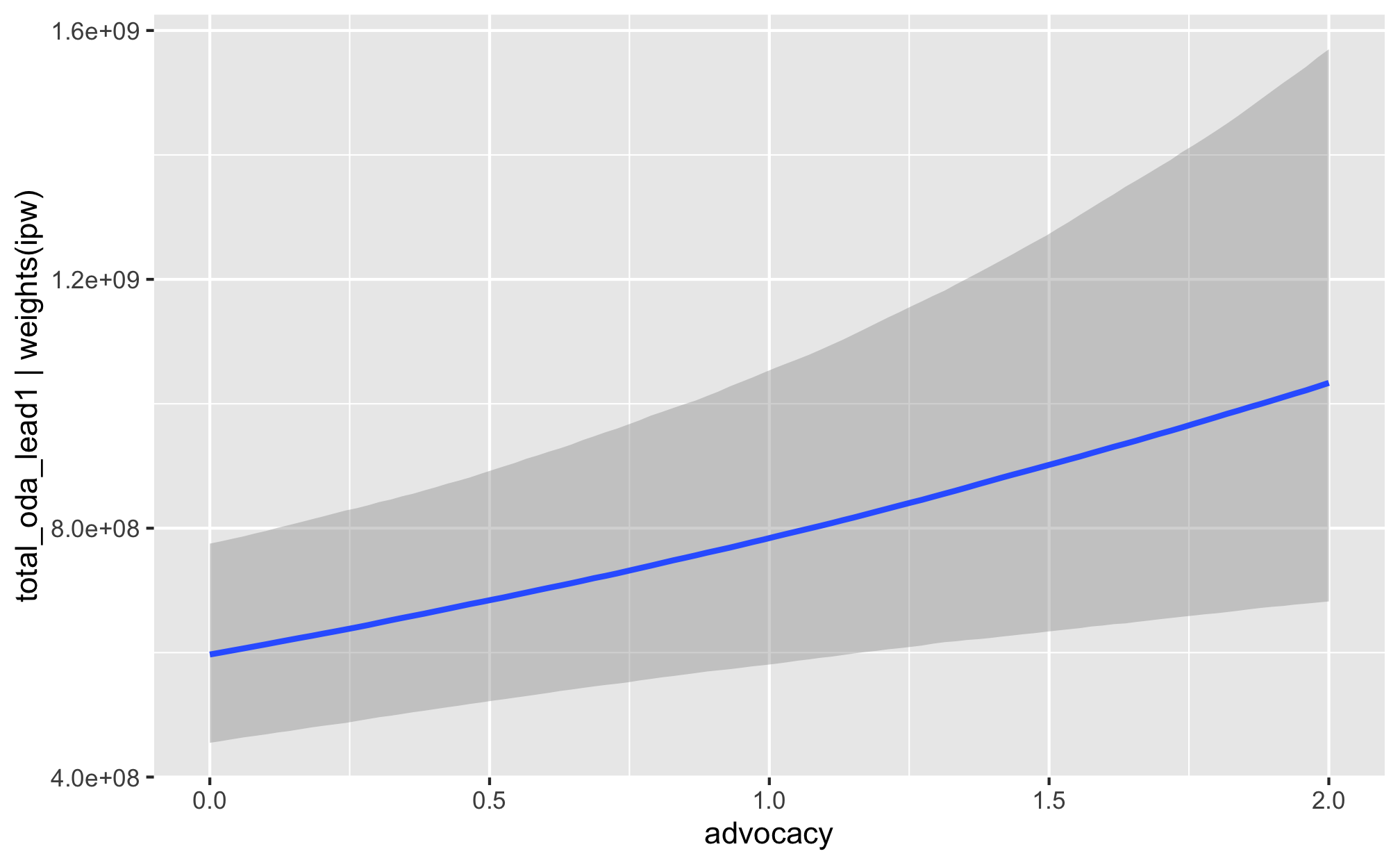

fit_h1_outcomes %>% 
  filter(model_name == "h1_entry") %>% 
  pull(fit_outcome) %>% nth(1) %>% 
  conditional_effects()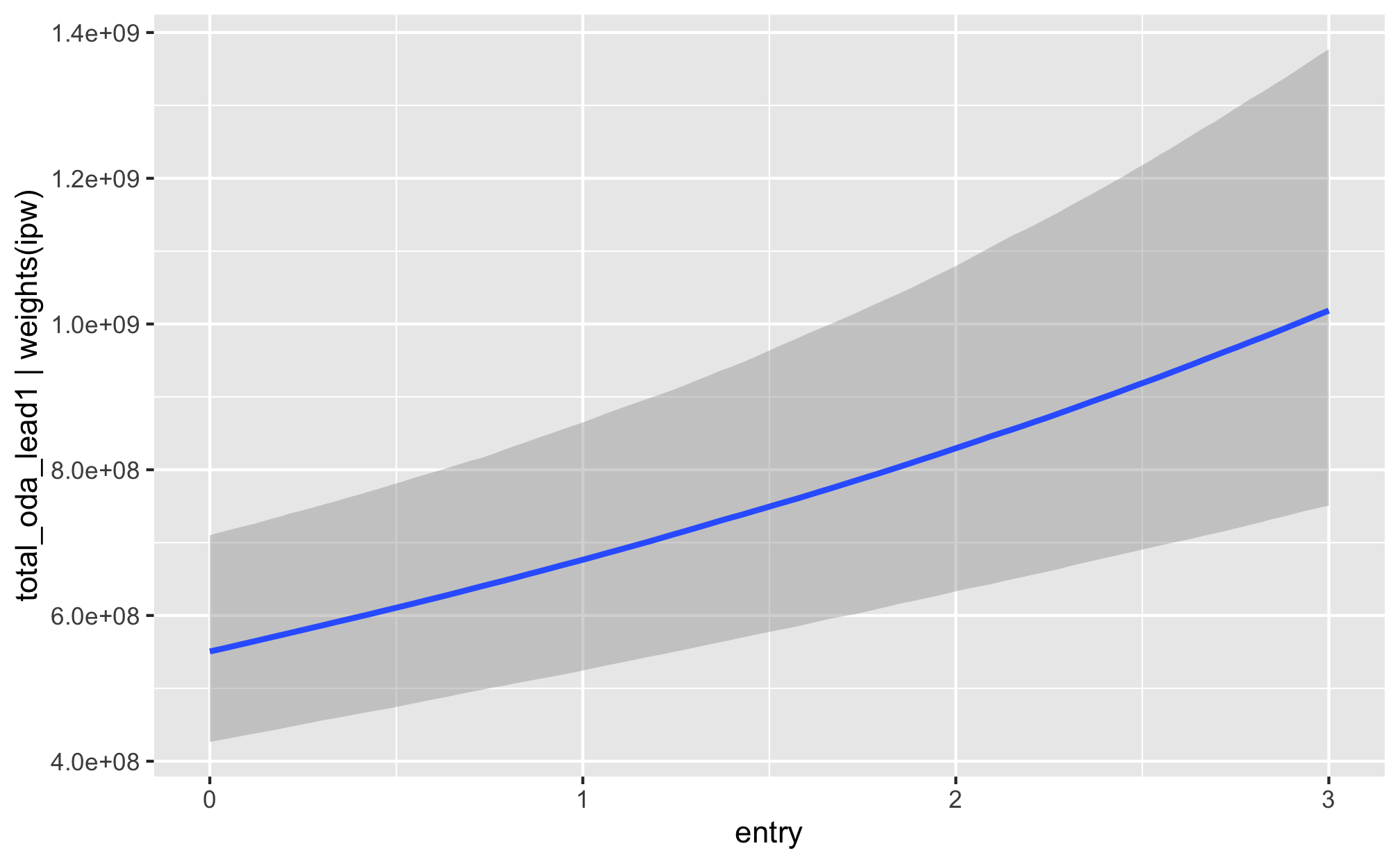

fit_h1_outcomes %>% 
  filter(model_name == "h1_funding") %>% 
  pull(fit_outcome) %>% nth(1) %>% 
  conditional_effects()

Copyright © 2017–2021 Suparna Chaudhry and Andrew Heiss. Licensed under the MIT License. Code available on GitHub.