Final analysis for paper
Steven L. Peck and Andrew Heiss
Last run: September 12, 2020
knitr::opts_chunk$set(warning = FALSE)

library(tidyverse)     # CRAN v1.3.0
library(broom)         # [github::tidymodels/broom] v0.5.3.9000
library(randomForest)  # CRAN v4.6-14
library(ggstance)      # CRAN v0.3.3
library(ggtext)        # [github::wilkelab/ggtext] v0.1.0
library(gghalves)      # [github::erocoar/gghalves] v0.1.0
library(ggforce)       # CRAN v0.3.1
library(patchwork)     # CRAN v1.0.0
library(pander)        # CRAN v0.6.3
library(scales)        # CRAN v1.1.0
library(pluralize)     # [github::hrbrmstr/pluralize] v0.1.0
library(glue)          # CRAN v1.4.0
library(here)          # CRAN v0.1

# Disable dplyr's automatic ungrouping message
options(dplyr.summarise.inform = FALSE)

SEED <- 1234

sim_hl <- read_rds(here("data", "derived_data", "sim_hl.rds"))
sim_ls <- read_rds(here("data", "derived_data", "sim_ls.rds"))

sim_high <- sim_hl %>% filter(repp == "High")
sim_low <- sim_hl %>% filter(repp == "Low")

constraint_combo_outcomes_hl <- read_rds(here("data", "derived_data",
                                              "constraint_combo_outcomes_hl.rds")) %>%
  mutate(constraint_combo = str_replace(constraint_combo, "selectfor_d", "species_drift"),
         constraint_combo = str_replace(constraint_combo, "select", "selection"),
         constraint_combo = str_replace(constraint_combo, "compete", "competition"),
         constraint_combo = str_replace(constraint_combo, "disperse", "dispersal"))

constraint_combo_outcomes_ls <- read_rds(here("data", "derived_data",
                                              "constraint_combo_outcomes_ls.rds")) %>%
  mutate(constraint_combo = str_replace(constraint_combo, "selectfor_d", "species_drift"),
         constraint_combo = str_replace(constraint_combo, "select", "selection"),
         constraint_combo = str_replace(constraint_combo, "compete", "competition"),
         constraint_combo = str_replace(constraint_combo, "disperse", "dispersal"))

diff_hl_outcomes_full <- sim_hl %>%
  group_by(n_constraints_f) %>%
  nest() %>%
  mutate(fitness_test = map(data, ~t.test(landscape_fitness_linked ~ repp, data = .)),
         evenness_test = map(data, ~t.test(avg_evenness_t ~ repp, data = .)),
         richness_test = map(data, ~t.test(landscape_richness_mean ~ repp, data = .)),
         turnover_test = map(data, ~t.test(turnover_diff ~ repp, data = .))) %>%
  mutate_at(vars(ends_with("test")), list(tidy = ~map(., ~tidy(.)))) %>%
  mutate_at(vars(ends_with("tidy")), list(diff = ~map_dbl(., "estimate"),
                                          p.value = ~map_dbl(., "p.value"))) %>%
  ungroup()

diff_hl_outcomes_plot <- diff_hl_outcomes_full %>%
  select(-data, -ends_with("_test"), -ends_with("_tidy")) %>%
  pivot_longer(cols = -n_constraints_f) %>%
  mutate(name = str_replace(name, "_test_tidy_", "_")) %>%
  separate(name, into = c("outcome", "statistic"), sep = "_") %>%
  pivot_wider(names_from = "statistic") %>%
  mutate(sig = ifelse(p.value < 0.05, "*", ""),
         sig = ifelse(is.nan(p.value), "", sig)) %>%
  mutate(nice_diff = glue("∆ = {round(diff, 3)}{sig}")) %>%
  mutate(nice_diff = str_replace(nice_diff, "\\-", "−"))
theme_constraint <- function(base_size = 8, base_family = "DejaVu Sans Condensed") {
ret <- theme_bw(base_size, base_family) +
theme(plot.title = element_text(size = rel(1.1), face = "bold",
family = "DejaVu Sans Condensed"),
plot.subtitle = element_text(size = rel(0.8), face = "plain",
family = "DejaVu Sans Condensed"),
plot.caption = element_text(size = rel(0.8), color = "grey50", face = "plain",
family = "DejaVu Sans Condensed",
margin = ggplot2::margin(t = 5)),
panel.border = element_rect(color = "grey50", fill = NA, size = 0.15),
panel.spacing = unit(1, "lines"),
panel.grid.minor = element_blank(),
strip.text = element_text(size = rel(0.9), hjust = 0,
family = "DejaVu Sans Condensed", face = "bold"),
strip.background = element_rect(fill = "#ffffff", colour = NA),
axis.ticks = element_blank(),
axis.title.x = element_text(margin = ggplot2::margin(t = 5)),
axis.text = element_text(family = "DejaVu Sans Condensed", face = "plain"),
legend.key = element_blank(),
legend.text = element_text(size = rel(1), family = "DejaVu Sans Condensed",
face = "plain"),
legend.spacing = unit(0.1, "lines"),
legend.box.margin = ggplot2::margin(t = -0.5, unit = "lines"),
legend.margin = ggplot2::margin(t = 0),
legend.position = "bottom")
ret
}
# Colors from https://medialab.github.io/iwanthue/
# 6 colors, default palette, soft (k-means)
clrs <- list(
select = "#6295cd", # blue
selection = "#6295cd", # blue
compete = "#b3943f", # gold
competition = "#b3943f", # gold
catastrophe = "#9466c9", # purple
create_network = "#62a85b", # green
dispersal = "#c85990", # pink
disperse = "#c85990", # pink
selectfor_d = "#ca5d46", # reddish
species_drift = "#ca5d46", # reddish
grey = "#7f7f7f" # grey50
)
color_constraints <- function(df, constraint_col) {
df %>%
mutate(constraint_colored = {{constraint_col}}) %>%
mutate(constraint_colored =
str_replace_all(constraint_colored, "\\bselect\\b",
glue("<span style='color:{clrs$select}'>select</span>")),
constraint_colored =
str_replace_all(constraint_colored, "\\bselection\\b",
glue("<span style='color:{clrs$selection}'>selection</span>")),
constraint_colored =
str_replace_all(constraint_colored, "\\bcompete\\b",
glue("<span style='color:{clrs$compete}'>compete</span>")),
constraint_colored =
str_replace_all(constraint_colored, "\\bcompetition\\b",
glue("<span style='color:{clrs$competition}'>competition</span>")),
constraint_colored =
str_replace_all(constraint_colored, "\\bcatastrophe\\b",
glue("<span style='color:{clrs$catastrophe}'>catastrophe</span>")),
constraint_colored =
str_replace_all(constraint_colored, "\\bcreate_network\\b",
glue("<span style='color:{clrs$create_network}'>create_network</span>")),
constraint_colored =
str_replace_all(constraint_colored, "\\bdisperse\\b",
glue("<span style='color:{clrs$disperse}'>disperse</span>")),
constraint_colored =
str_replace_all(constraint_colored, "\\bdispersal\\b",
glue("<span style='color:{clrs$dispersal}'>dispersal</span>")),
constraint_colored =
str_replace_all(constraint_colored, "\\bselectfor_d\\b",
glue("<span style='color:{clrs$selectfor_d}'>selectfor_d</span>")),
constraint_colored =
str_replace_all(constraint_colored, "\\bspecies_drift\\b",
glue("<span style='color:{clrs$species_drift}'>species_drift</span>")))
}
# Function for plotting outcomes across combinations of constraints
mega_means_plot <- function(df, var_name, xlab, title, add_to_right = 0, add_to_left = 0.03, xlim = NULL) {
constraint_combos <- df %>%
group_by(constraint_combo, n) %>%
summarize(avg = mean({{var_name}})) %>%
arrange(desc(n), desc(avg)) %>%
ungroup() %>%
mutate(constraint_combo = ifelse(n >= 4,
str_wrap(constraint_combo, width = 40, exdent = 8),
constraint_combo)) %>%
mutate(constraint_combo = str_replace_all(constraint_combo, " {8}", "<br>")) %>%
mutate(constraint_combo = recode(constraint_combo,
`select` = "selection",
`compete` = "competition",
`disperse` = "dispersal",
`selectfor_d` = "species_drift")) %>%
color_constraints(constraint_combo) %>%
mutate(constraint_colored = fct_inorder(constraint_colored),
n_title = map_chr(n, ~paste0(., pluralize(" constraint", .))))
plot_02 <- ggplot(filter(constraint_combos, n %in% c(0, 1, 2)),
aes(x = avg, y = constraint_colored)) +
geom_pointrangeh(aes(xmin = 0, xmax = avg)) +
scale_x_continuous(expand = expansion(add = c(add_to_right, add_to_left))) +
labs(x = xlab, y = NULL) +
facet_col(vars(n_title), scales = "free_y", space = "free") +
theme_constraint() +
theme(axis.text.y = element_markdown(),
panel.grid.major.y = element_blank(),
strip.background = element_rect(fill = "grey80"))
plot_3 <- ggplot(filter(constraint_combos, n == 3),
aes(x = avg, y = constraint_colored)) +
geom_pointrangeh(aes(xmin = 0, xmax = avg)) +
scale_x_continuous(expand = expansion(add = c(add_to_right, add_to_left))) +
labs(x = xlab, y = NULL) +
facet_col(vars(n_title), scales = "free_y", space = "free") +
theme_constraint() +
theme(axis.text.y = element_markdown(),
panel.grid.major.y = element_blank(),
strip.background = element_rect(fill = "grey80"))
plot_46 <- ggplot(filter(constraint_combos, n %in% c(4, 5, 6)),
aes(x = avg, y = constraint_colored)) +
geom_pointrangeh(aes(xmin = 0, xmax = avg)) +
scale_x_continuous(expand = expansion(add = c(add_to_right, add_to_left))) +
labs(x = xlab, y = NULL) +
facet_col(vars(n_title), scales = "free_y", space = "free") +
theme_constraint() +
theme(axis.text.y = element_markdown(),
panel.grid.major.y = element_blank(),
strip.background = element_rect(fill = "grey80"))
if (!is.null(xlim)) {
plot_02 <- plot_02 + coord_cartesian(xlim = xlim)
plot_3 <- plot_3 + coord_cartesian(xlim = xlim)
plot_46 <- plot_46 + coord_cartesian(xlim = xlim)
}
plot_all <- (plot_02 | plot_3 | plot_46) +
plot_annotation(title = title,
theme = theme(plot.title = element_text(size = rel(1.1), face = "bold",
family = "DejaVu Sans Condensed")))
plot_all
}Variable importance
To determine which constraints matter the most, we use random forests to determine variable importance. We don’t need to include all the interactions (e.g. create_network + select + create_network * select, etc.) because random forests inherently pick those up.
There are two ways to measure variable importance with random forests: (1) Gini-based node impurity, and (2) permutation-based increase in mean standard error. Gini-based node impurity is trickier to interpret. According to Liz Dinsdale:
The mean decrease in Gini coefficient is a measure of how each variable contributes to the homogeneity of the nodes and leaves in the resulting random forest. Each time a particular variable is used to split a node, the Gini coefficient for the child nodes are calculated and compared to that of the original node. The Gini coefficient is a measure of homogeneity from 0 (homogeneous) to 1 (heterogeneous). The changes in Gini are summed for each variable and normalized at the end of the calculation. Variables that result in nodes with higher purity have a higher decrease in Gini coefficient.
Or in other words, importance is the mean decrease (over all the trees) in the Gini index by splits of a predictor. Basically, the higher the decrease in impurity, the more important the variable in explaining the outcome.
However, node impurity tends to inflate or distort variable importance for continuous variables, and it uses the entire data set. A common alternative (that is also more interpretable!) is to look at the percent increase in mean standard error (see slide 15 here and this answer here). This measures how much the model’s MSE changes if you shuffle one of the variables (i.e. if you completely shuffle select, how wrong does the model become?). High values show that the variable is important for maintaining accuracy; low values show that the variable doesn’t matter all that much (since it can be random noise and result in similar accuracy). Like here, the Gini-based version finds that passenger ID is incredibly important for predicting survival on the Titanic, when really it’s just a random variable that doesn’t matter. The percent-change-in-MSE-based version of importance isn’t fooled by passenger ID, though.
Because of that, we use mean decrease in accuracy as our measure of variable importance.
library(titanic)  # CRAN v0.1.0
titanic <- titanic::titanic_train %>%
  drop_na() %>%
  mutate(Sex = as.factor(Sex), Survived = as.factor(Survived), Pclass = as.factor(Pclass))

set.seed(SEED)
titanic_forest <- randomForest(Survived ~ Age + Sex + Pclass + PassengerId,
                               data = titanic, importance = TRUE)
varImpPlot(titanic_forest)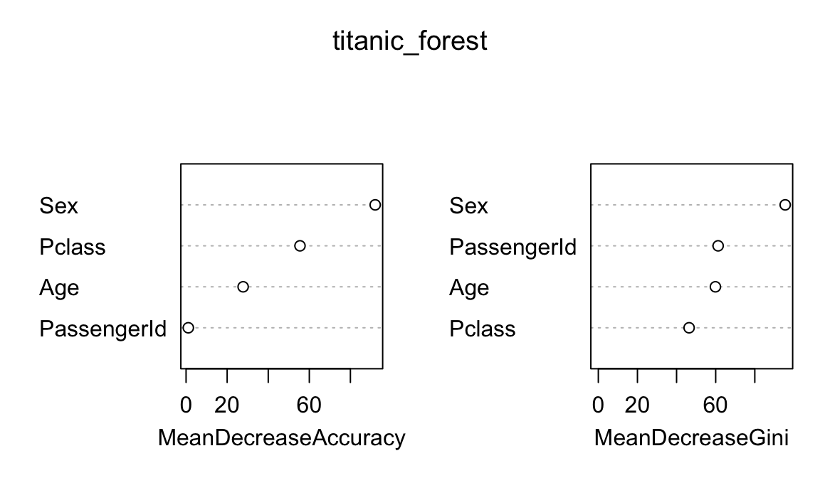
Figures
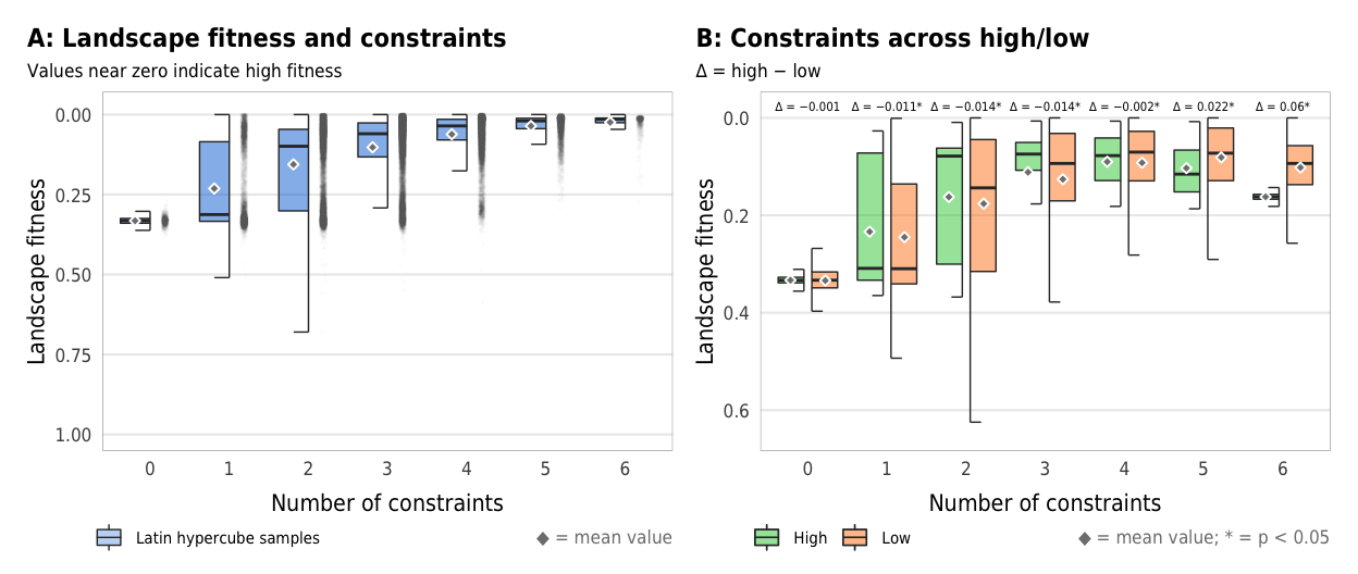
Figure 4: Landscape fitness
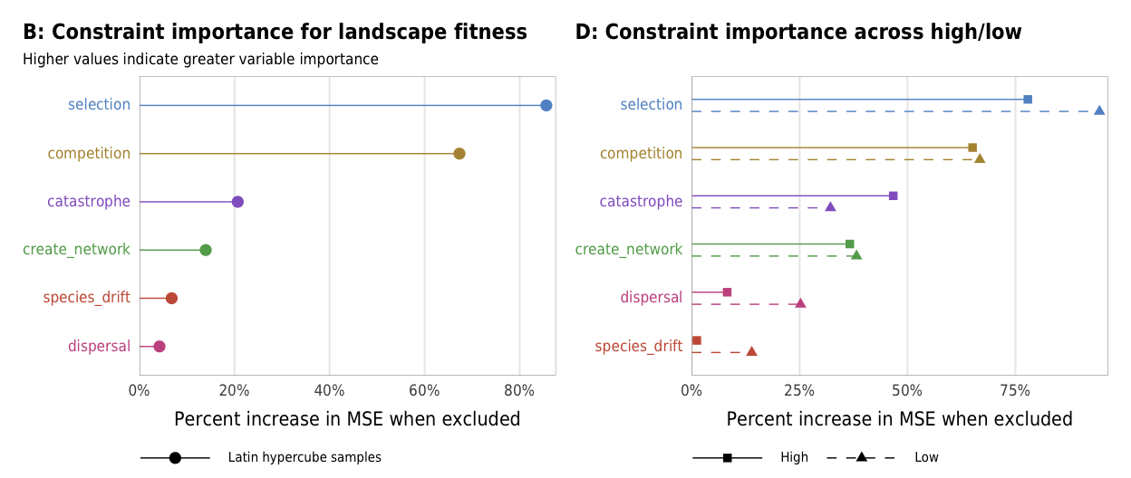
Fig 4. Effect of the number of constraints on landscape fitness (A) Boxplots showing landscape fitness across different numbers of constraints; (B) Percent increase in mean standard error in a random forest model when each constraint is removed; (C) Average landscape fitness across all possible combinations of constraints
plot_fitness_boxplot <- ggplot(sim_ls, aes(x = n_constraints_f, y = landscape_fitness_linked)) +
  geom_half_point(size = 0.01, alpha = 0.01, side = "r", color = "grey50",
                  transformation_params = list(width = 0.25, height = 0, seed = 1234)) +
  geom_half_boxplot(aes(fill = "Latin hypercube samples"),
                    size = 0.25, side = "l", outlier.shape = NA, errorbar.draw = TRUE, alpha = 0.5) +
  stat_summary(geom = "point", fun = "mean",
               size = 1, pch = 23, fill = clrs$grey, color = "white",
               position = position_nudge(x = -0.19)) +
  scale_y_reverse() +
  scale_fill_manual(values = c("#0074D9"), name = NULL) +
  guides(fill = guide_legend(direction = "horizontal", override.aes = list(alpha = 0.3, size = 0.25))) +
  coord_cartesian(ylim = c(1, -0.02)) +
  labs(x = "Number of constraints",
       y = "Landscape fitness",
       title = "A: Landscape fitness and constraints",
       subtitle = "Values near zero indicate high fitness",
       caption = glue("<span style='color:{clrs$grey}'>◆</span> = mean value")) +
  theme_constraint() +
  theme(panel.grid.major.x = element_blank(),
        plot.caption = element_markdown(),
        plot.title.position = "plot",
        legend.position = c(0, 0),
        legend.justification = "left",
        legend.text = element_text(size = rel(0.7)),
        legend.box.margin = ggplot2::margin(l = -0.5, t = 4.15, unit = "lines"),
        legend.key.size = unit(0.75, "lines"))
plot_fitness_boxplot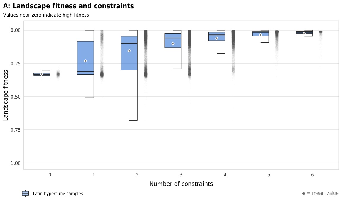
ggsave(plot_fitness_boxplot, filename = here("analysis", "output", "fitness_A.pdf"),
       width = params$fig_width, height = params$fig_height, units = "in", device = cairo_pdf)
ggsave(plot_fitness_boxplot, filename = here("analysis", "output", "fitness_A.png"),
       width = params$fig_width, height = params$fig_height, units = "in", type = "cairo", dpi = 300)
plot_fitness_hl_diffs <- ggplot(mapping = aes(x = n_constraints_f, y = landscape_fitness_linked, fill = repp)) +
geom_text(data = filter(diff_hl_outcomes_plot, outcome == "fitness"),
aes(y = 0, label = nice_diff, fill = NULL),
family = "DejaVu Sans Condensed", fontface = "plain", size = 1.5, vjust = -0.85) +
geom_half_boxplot(data = sim_high,
size = 0.25, side = "l", outlier.shape = NA, errorbar.draw = TRUE,
nudge = 0.05, alpha = 0.5) +
geom_half_boxplot(data = sim_low,
size = 0.25, side = "r", outlier.shape = NA, errorbar.draw = TRUE,
nudge = 0.05, alpha = 0.5) +
stat_summary(data = sim_high, geom = "point", fun = "mean",
size = 1, pch = 23, fill = clrs$grey, color = "white",
position = position_nudge(x = -0.22)) +
stat_summary(data = sim_low, geom = "point", fun = "mean",
size = 1, pch = 23, fill = clrs$grey, color = "white",
position = position_nudge(x = 0.22)) +
scale_y_reverse() +
scale_fill_manual(values = c("#2ECC40", "#FF851B"), name = NULL) +
guides(fill = guide_legend(direction = "horizontal", override.aes = list(alpha = 0.3, size = 0.25))) +
coord_cartesian(ylim = c(0.65, -0.02)) +
labs(x = "Number of constraints",
y = "Landscape fitness",
title = "B: Constraints across high/low",
subtitle = "∆ = high − low",
caption = glue("<span style='color:{clrs$grey}'>◆</span> = mean value; * = p < 0.05")) +
theme_constraint() +
theme(panel.grid.major.x = element_blank(),
plot.caption = element_markdown(),
plot.title.position = "plot",
legend.position = c(0, 0),
legend.justification = "left",
legend.text = element_text(size = rel(0.7)),
legend.box.margin = ggplot2::margin(l = -0.5, t = 4.15, unit = "lines"),
legend.key.size = unit(0.75, "lines"))
plot_fitness_hl_diffs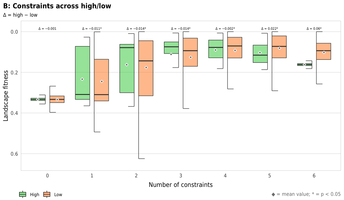
ggsave(combined_fitness, filename = here("analysis", "output", "fitness_boxplots.pdf"),
       width = params$fig_width2, height = params$fig_height, units = "in", device = cairo_pdf)
ggsave(combined_fitness, filename = here("analysis", "output", "fitness_boxplots.png"),
       width = params$fig_width2, height = params$fig_height, units = "in", type = "cairo", dpi = 300)
# ggsave(combined_fitness, filename = here("analysis", "output", "fitness_combined.eps"),
#        width = params$fig_width2, height = params$fig_height, units = "in", device = cairo_ps, fallback_resolution = 600)
# This takes a few minutes to run
set.seed(SEED)
forest_model_fitness <-
randomForest(landscape_fitness_linked ~
create_network + select + disperse +
compete + selectfor_d + catastrophe,
importance = TRUE, data = sim_ls)
forest_model_fitness_low <-
randomForest(landscape_fitness_linked ~
create_network + select + disperse +
compete + selectfor_d + catastrophe,
importance = TRUE, data = filter(sim_hl, repp == "Low"))
forest_model_fitness_high <-
randomForest(landscape_fitness_linked ~
create_network + select + disperse +
compete + selectfor_d + catastrophe,
importance = TRUE, data = filter(sim_hl, repp == "High"))clrs <- list(
select = "#6295cd", # blue
selection = "#6295cd", # blue
compete = "#b3943f", # gold
competition = "#b3943f", # gold
catastrophe = "#9466c9", # purple
create_network = "#62a85b", # green
dispersal = "#c85990", # pink
disperse = "#c85990", # pink
selectfor_d = "#ca5d46", # reddish
species_drift = "#ca5d46", # reddish
grey = "#7f7f7f" # grey50
)
fitness_importance_ls <- importance(forest_model_fitness, type = 1, scale = TRUE) %>%
data.frame() %>%
rownames_to_column(var = "constraint") %>%
arrange(desc(X.IncMSE)) %>%
mutate(constraint = recode(constraint,
`select` = "selection",
`compete` = "competition",
`disperse` = "dispersal",
`selectfor_d` = "species_drift")) %>%
color_constraints(constraint) %>%
mutate_at(vars(starts_with("constraint")), fct_inorder) %>%
mutate(X.IncMSE = X.IncMSE / 100)
plot_fitness_importance_ls <- ggplot(fitness_importance_ls,
aes(x = X.IncMSE, y = fct_rev(constraint_colored),
color = fct_rev(constraint),
shape = "Latin hypercube samples")) +
geom_pointrangeh(aes(xmin = 0, xmax = X.IncMSE), size = 0.25) +
scale_x_continuous(labels = percent, expand = expansion(add = c(0, 0.02))) +
scale_color_manual(values = unlist(clrs), guide = FALSE) +
scale_shape_manual(values = c(19), name = NULL) +
guides(shape = guide_legend(direction = "horizontal",
override.aes = list(size = 0.25))) +
labs(x = "Percent increase in MSE when excluded", y = NULL,
title = "B: Constraint importance for landscape fitness",
subtitle = "Higher values indicate greater variable importance",
caption = "") +
theme_constraint() +
theme(panel.grid.major.y = element_blank(),
axis.text.y = element_markdown(),
plot.title.position = "plot",
legend.position = c(0, 0),
legend.justification = "left",
legend.text = element_markdown(size = rel(0.7)),
legend.box.margin = ggplot2::margin(l = -0.5, t = 4.75, unit = "lines"),
legend.key.width = unit(2.5, "lines"),
legend.key.size = unit(0.95, "lines"))
plot_fitness_importance_ls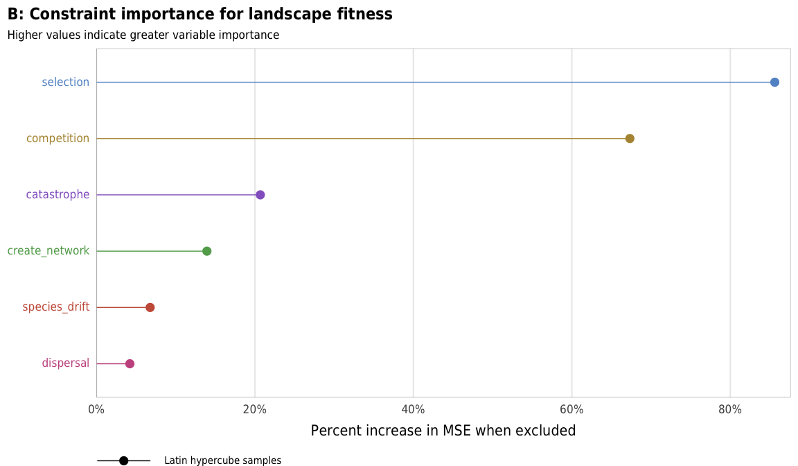
ggsave(plot_fitness_importance_ls, filename = here("analysis", "output", "fitness_B.pdf"),
       width = params$fig_width, height = params$fig_height, units = "in", device = cairo_pdf)
ggsave(plot_fitness_importance_ls, filename = here("analysis", "output", "fitness_B.png"),
       width = params$fig_width, height = params$fig_height, units = "in", type = "cairo", dpi = 300)
fitness_importance_low <- importance(forest_model_fitness_low, type = 1, scale = TRUE) %>%
data.frame() %>%
rownames_to_column(var = "constraint") %>%
mutate(repp = "Low")
fitness_importance_high <- importance(forest_model_fitness_high, type = 1, scale = TRUE) %>%
data.frame() %>%
rownames_to_column(var = "constraint") %>%
mutate(repp = "High")
fitness_importance_hl <- bind_rows(fitness_importance_low,
fitness_importance_high) %>%
mutate(repp = factor(repp, levels = c("Low", "High"), ordered = TRUE)) %>%
arrange(desc(repp), desc(X.IncMSE)) %>%
mutate(constraint = recode(constraint,
`select` = "selection",
`compete` = "competition",
`disperse` = "dispersal",
`selectfor_d` = "species_drift")) %>%
color_constraints(constraint) %>%
mutate_at(vars(starts_with("constraint")), fct_inorder) %>%
mutate(X.IncMSE = X.IncMSE / 100)
plot_fitness_importance_hl <- ggplot(fitness_importance_hl,
aes(x = X.IncMSE, y = fct_rev(constraint_colored), color = fct_rev(constraint),
linetype = repp, shape = repp)) +
geom_pointrangeh(aes(xmin = 0, xmax = X.IncMSE),
position = position_dodgev(height = 0.5), size = 0.25) +
scale_x_continuous(labels = percent, expand = expansion(add = c(0, 0.02))) +
scale_color_manual(values = unlist(clrs), guide = FALSE) +
scale_linetype_manual(values = c("dashed", "solid"), name = NULL) +
scale_shape_manual(values = c(17, 15), name = NULL) +
guides(linetype = guide_legend(direction = "horizontal", reverse = TRUE),
shape = guide_legend(direction = "horizontal", override.aes = list(size = 0.25),
reverse = TRUE)) +
labs(x = "Percent increase in MSE when excluded", y = NULL,
title = "D: Constraint importance across high/low",
subtitle = "",
caption = "") +
theme_constraint() +
theme(panel.grid.major.y = element_blank(),
axis.text.y = element_markdown(),
plot.title.position = "plot",
legend.position = c(0, 0),
legend.justification = "left",
legend.text = element_markdown(size = rel(0.7)),
legend.box.margin = ggplot2::margin(l = -0.5, t = 4.75, unit = "lines"),
legend.key.width = unit(2.5, "lines"),
legend.key.size = unit(0.95, "lines"))
plot_fitness_importance_hl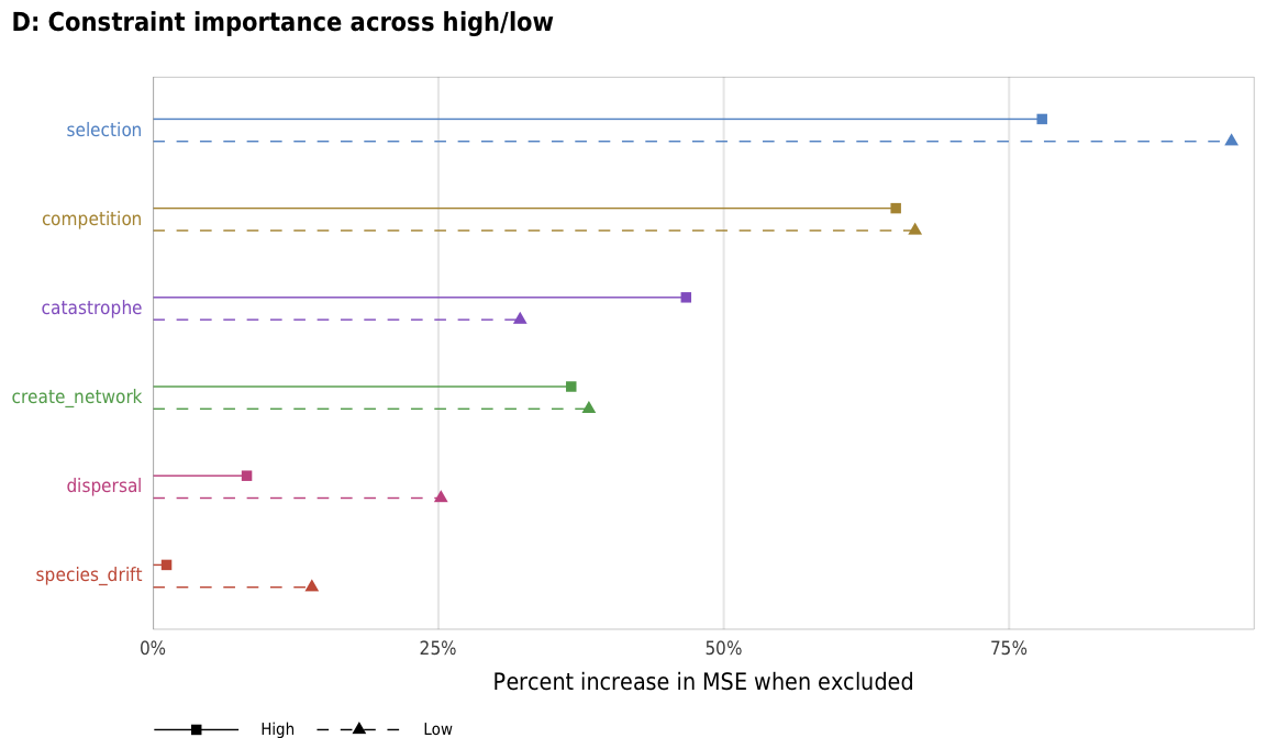
ggsave(importance_fitness, filename = here("analysis", "output", "fitness_importance.pdf"),
       width = params$fig_width2, height = params$fig_height, units = "in", device = cairo_pdf)
ggsave(importance_fitness, filename = here("analysis", "output", "fitness_importance.png"),
       width = params$fig_width2, height = params$fig_height, units = "in", type = "cairo", dpi = 300)
# ggsave(combined_fitness, filename = here("analysis", "output", "fitness_combined.tiff"),
#        width = params$fig_width2, height = params$fig_height, units = "in", type = "cairo", dpi = 600)
# ggsave(combined_fitness, filename = here("analysis", "output", "fitness_combined.eps"),
#        width = params$fig_width2, height = params$fig_height, units = "in", device = cairo_ps, fallback_resolution = 600)
plot_fitness_all <- mega_means_plot(constraint_combo_outcomes_ls, landscape_fitness_linked,
xlab = "Average landscape fitness",
title = "Average landscape fitness across combinations of constraints")
plot_fitness_all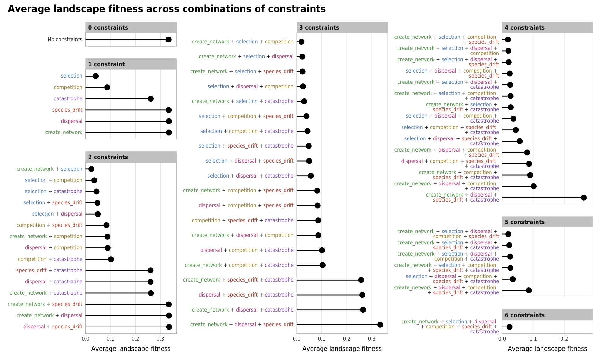
ggsave(plot_fitness_all, filename = here("analysis", "output", "fitness_means_all.pdf"),
       width = params$fig_width_big, height = params$fig_height_big, units = "in", device = cairo_pdf)
ggsave(plot_fitness_all, filename = here("analysis", "output", "fitness_means_all.png"),
       width = params$fig_width_big, height = params$fig_height_big, units = "in", type = "cairo", dpi = 300)
Figure 5: Landscape fitness variance
Fig 5. Effect of the number of constraints on variance of landscape fitness Boxplots showing variance of landscape fitness across different numbers of constraints
plot_landscape_fitness_variance <- ggplot(sim_ls,
                                          aes(x = n_constraints_f, y = landscape_fitness_var)) +
  geom_half_point(size = 0.05, alpha = 0.1, side = "r", color = "grey50",
                  transformation_params = list(width = 0.25, height = 0, seed = 1234)) +
  geom_half_boxplot(size = 0.25, side = "l", outlier.shape = NA, errorbar.draw = TRUE) +
  stat_summary(geom = "point", fun = "mean",
               size = 1, pch = 23, fill = clrs$grey, color = "white",
               position = position_nudge(x = -0.19)) +
  scale_y_reverse() +
  coord_cartesian(ylim = c(0.1, 0)) +
  labs(x = "Number of constraints",
       y = "Landscape fitness, variance",
       title = "Variance in landscape fitness and constraints",
       subtitle = "Latin hypercube samples",
       caption = glue("<span style='color:{clrs$grey}'>◆</span> = mean value")) +
  theme_constraint() +
  theme(panel.grid.major.x = element_blank(),
        plot.caption = element_markdown())

plot_landscape_fitness_variance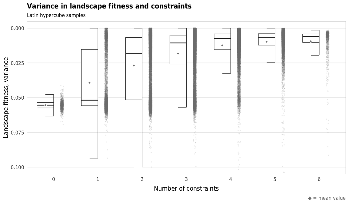
ggsave(plot_landscape_fitness_variance, filename = here("analysis", "output", "fitness_variance.pdf"),
       width = params$fig_width, height = params$fig_height, units = "in", device = cairo_pdf)
ggsave(plot_landscape_fitness_variance, filename = here("analysis", "output", "fitness_variance.png"),
       width = params$fig_width, height = params$fig_height, units = "in", type = "cairo", dpi = 300)
Figure 6: Ecological evenness
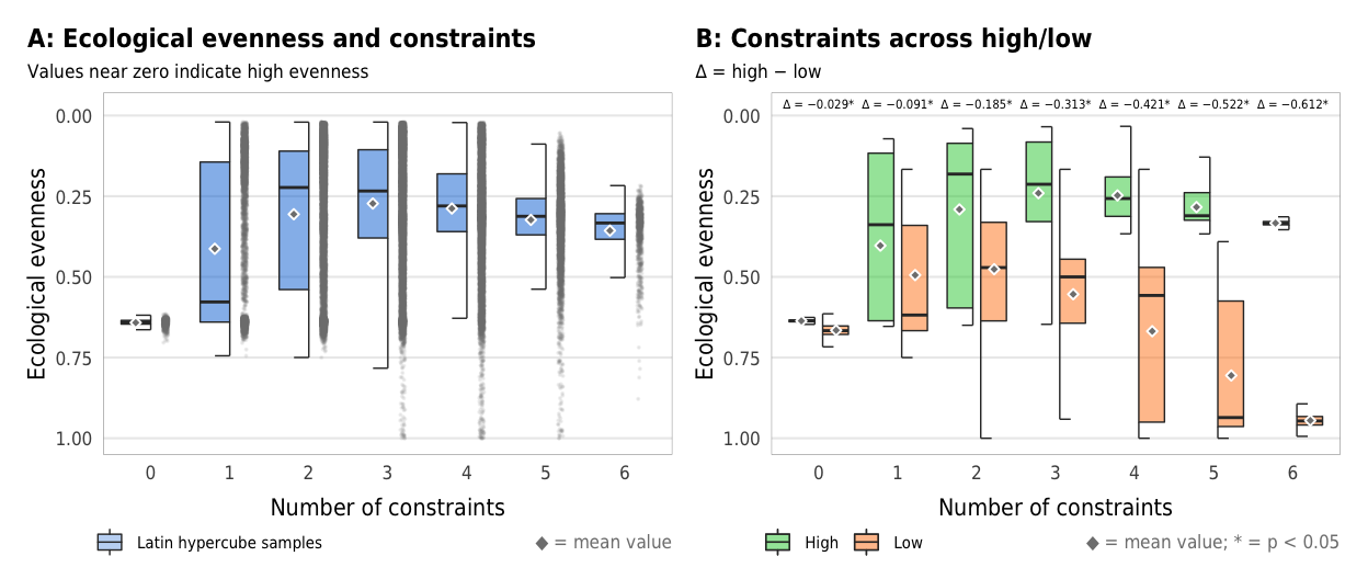
Fig 6. Effect of the number of constraints on ecological evenness (A) Boxplots showing ecological evenness across different numbers of constraints; (B) Percent increase in mean standard error in a random forest model when each constraint is removed; (C) Average ecological evenness across all possible combinations of constraints
plot_evenness_boxplot <- ggplot(sim_ls, aes(x = n_constraints_f, y = avg_evenness_t)) +
  geom_half_point(size = 0.05, alpha = 0.1, side = "r", color = "grey50",
                  transformation_params = list(width = 0.25, height = 0, seed = 1234)) +
  geom_half_boxplot(aes(fill = "Latin hypercube samples"),
                    size = 0.25, side = "l", outlier.shape = NA, errorbar.draw = TRUE, alpha = 0.5) +
  stat_summary(geom = "point", fun = "mean",
               size = 1, pch = 23, fill = clrs$grey, color = "white",
               position = position_nudge(x = -0.19)) +
  scale_y_reverse() +
  scale_fill_manual(values = c("#0074D9"), name = NULL) +
  guides(fill = guide_legend(direction = "horizontal", override.aes = list(alpha = 0.3, size = 0.25))) +
  coord_cartesian(ylim = c(1, -0.02)) +
  labs(x = "Number of constraints",
       y = "Ecological evenness",
       title = "A: Ecological evenness and constraints",
       subtitle = "Values near zero indicate high evenness",
       caption = glue("<span style='color:{clrs$grey}'>◆</span> = mean value")) +
  theme_constraint() +
  theme(panel.grid.major.x = element_blank(),
        plot.caption = element_markdown(),
        plot.title.position = "plot",
        legend.position = c(0, 0),
        legend.justification = "left",
        legend.text = element_text(size = rel(0.7)),
        legend.box.margin = ggplot2::margin(l = -0.5, t = 4.15, unit = "lines"),
        legend.key.size = unit(0.75, "lines"))
plot_evenness_boxplot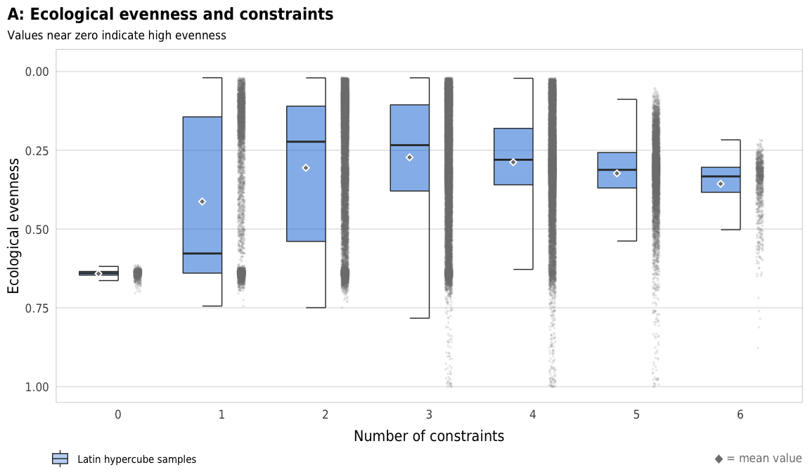
ggsave(plot_evenness_boxplot, filename = here("analysis", "output", "evenness_A.pdf"),
       width = params$fig_width, height = params$fig_height, units = "in", device = cairo_pdf)
ggsave(plot_evenness_boxplot, filename = here("analysis", "output", "evenness_A.png"),
       width = params$fig_width, height = params$fig_height, units = "in", type = "cairo", dpi = 300)
plot_evenness_hl_diffs <- ggplot(mapping = aes(x = n_constraints_f, y = avg_evenness_t, fill = repp)) +
geom_text(data = filter(diff_hl_outcomes_plot, outcome == "evenness"),
aes(y = 0, label = nice_diff, fill = NULL),
family = "DejaVu Sans Condensed", fontface = "plain", size = 1.5, vjust = -0.85) +
geom_half_boxplot(data = sim_high,
size = 0.25, side = "l", outlier.shape = NA, errorbar.draw = TRUE,
nudge = 0.05, alpha = 0.5) +
geom_half_boxplot(data = sim_low,
size = 0.25, side = "r", outlier.shape = NA, errorbar.draw = TRUE,
nudge = 0.05, alpha = 0.5) +
stat_summary(data = sim_high, geom = "point", fun = "mean",
size = 1, pch = 23, fill = clrs$grey, color = "white",
position = position_nudge(x = -0.22)) +
stat_summary(data = sim_low, geom = "point", fun = "mean",
size = 1, pch = 23, fill = clrs$grey, color = "white",
position = position_nudge(x = 0.22)) +
scale_y_reverse() +
scale_fill_manual(values = c("#2ECC40", "#FF851B"), name = NULL) +
guides(fill = guide_legend(direction = "horizontal", override.aes = list(alpha = 0.3, size = 0.25))) +
coord_cartesian(ylim = c(1, -0.02)) +
labs(x = "Number of constraints",
y = "Ecological evenness",
title = "B: Constraints across high/low",
subtitle = "∆ = high − low",
caption = glue("<span style='color:{clrs$grey}'>◆</span> = mean value; * = p < 0.05")) +
theme_constraint() +
theme(panel.grid.major.x = element_blank(),
plot.caption = element_markdown(),
plot.title.position = "plot",
legend.position = c(0, 0),
legend.justification = "left",
legend.text = element_text(size = rel(0.7)),
legend.box.margin = ggplot2::margin(l = -0.5, t = 4.15, unit = "lines"),
legend.key.size = unit(0.75, "lines"))
plot_evenness_hl_diffs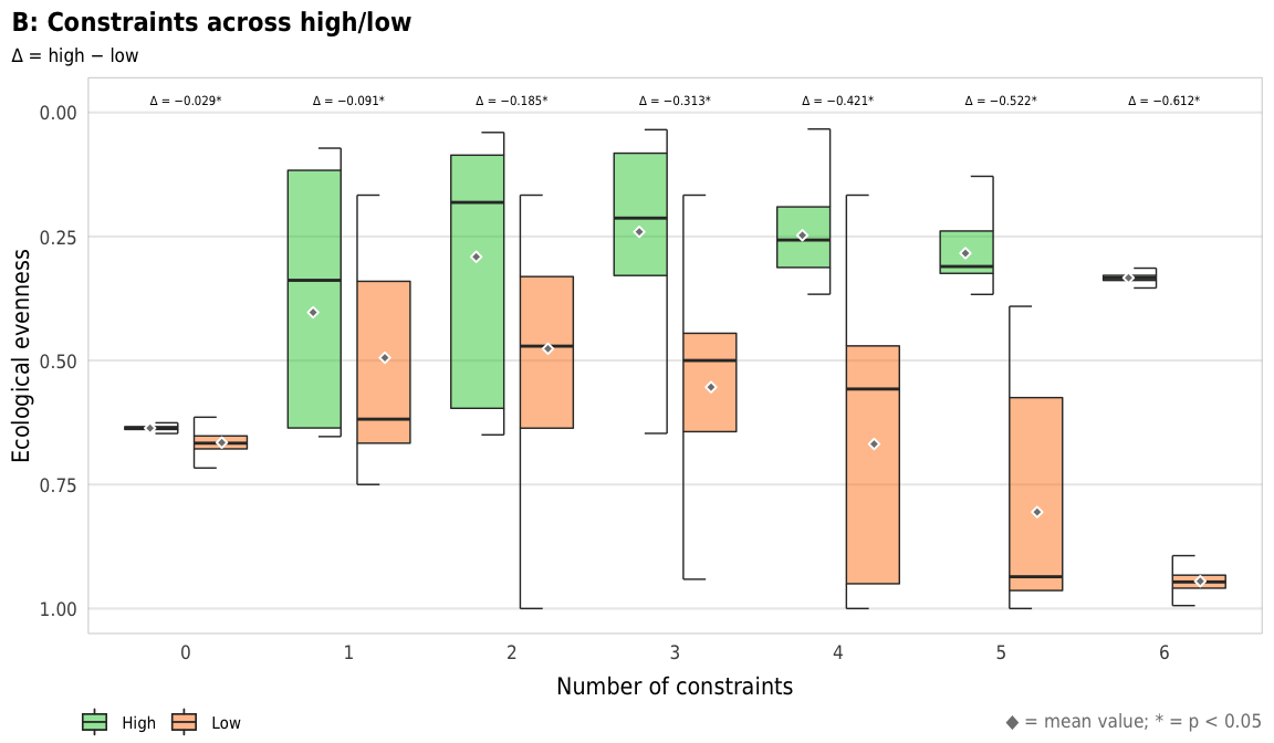
ggsave(combined_evenness, filename = here("analysis", "output", "evenness_boxplots.pdf"),
       width = params$fig_width2, height = params$fig_height, units = "in", device = cairo_pdf)
ggsave(combined_evenness, filename = here("analysis", "output", "evenness_boxplots.png"),
       width = params$fig_width2, height = params$fig_height, units = "in", type = "cairo", dpi = 300)
# ggsave(combined_evenness, filename = here("analysis", "output", "evenness_combined.tiff"),
#        width = params$fig_width2, height = params$fig_height, units = "in", type = "cairo", dpi = 600)
# ggsave(combined_evenness, filename = here("analysis", "output", "evenness_combined.eps"),
#        width = params$fig_width2, height = params$fig_height, units = "in", device = cairo_ps, fallback_resolution = 600)
# This takes a few minutes to run
set.seed(SEED)
forest_model_evenness <-
randomForest(avg_evenness_t ~
create_network + select + disperse +
compete + selectfor_d + catastrophe,
importance = TRUE,
data = drop_na(sim_ls, avg_evenness_t))
forest_model_evenness_low <-
randomForest(avg_evenness_t ~
create_network + select + disperse +
compete + selectfor_d + catastrophe,
importance = TRUE,
data = filter(drop_na(sim_hl, avg_evenness_t), repp == "Low"))
forest_model_evenness_high <-
randomForest(avg_evenness_t ~
create_network + select + disperse +
compete + selectfor_d + catastrophe,
importance = TRUE,
data = filter(drop_na(sim_hl, avg_evenness_t), repp == "High"))evenness_importance_ls <- importance(forest_model_evenness, type = 1, scale = TRUE) %>%
data.frame() %>%
rownames_to_column(var = "constraint") %>%
arrange(desc(X.IncMSE)) %>%
mutate(constraint = recode(constraint,
`select` = "selection",
`compete` = "competition",
`disperse` = "dispersal",
`selectfor_d` = "species_drift")) %>%
color_constraints(constraint) %>%
mutate_at(vars(starts_with("constraint")), fct_inorder) %>%
mutate(X.IncMSE = X.IncMSE / 100)
plot_evenness_importance_ls <- ggplot(evenness_importance_ls,
aes(x = X.IncMSE, y = fct_rev(constraint_colored),
color = fct_rev(constraint), shape = "Latin hypercube samples")) +
geom_pointrangeh(aes(xmin = 0, xmax = X.IncMSE), size = 0.25) +
scale_x_continuous(labels = percent, expand = expansion(add = c(0, 0.02))) +
scale_color_manual(values = unlist(clrs), guide = FALSE) +
scale_shape_manual(values = c(19), name = NULL) +
guides(shape = guide_legend(direction = "horizontal",
override.aes = list(size = 0.25))) +
labs(x = "Percent increase in MSE when excluded", y = NULL,
title = "B: Constraint importance for ecological evenness",
subtitle = "Higher values indicate greater variable importance",
caption = "") +
theme_constraint() +
theme(panel.grid.major.y = element_blank(),
axis.text.y = element_markdown(),
plot.title.position = "plot",
legend.position = c(0, 0),
legend.justification = "left",
legend.text = element_markdown(size = rel(0.7)),
legend.box.margin = ggplot2::margin(l = -0.5, t = 4.75, unit = "lines"),
legend.key.width = unit(2.5, "lines"),
legend.key.size = unit(0.95, "lines"))
plot_evenness_importance_ls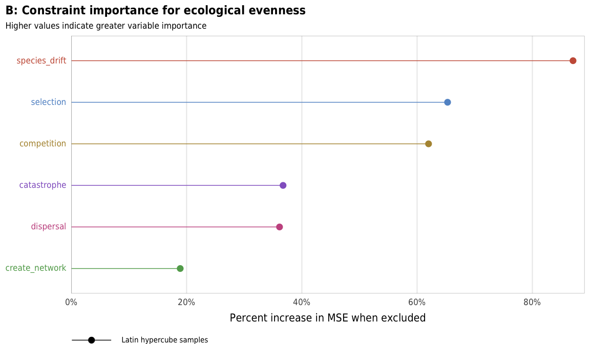
ggsave(plot_evenness_importance_ls, filename = here("analysis", "output", "evenness_B.pdf"),
       width = params$fig_width, height = params$fig_height, units = "in", device = cairo_pdf)
ggsave(plot_evenness_importance_ls, filename = here("analysis", "output", "evenness_B.png"),
       width = params$fig_width, height = params$fig_height, units = "in", type = "cairo", dpi = 300)
evenness_importance_low <- importance(forest_model_evenness_low, type = 1, scale = TRUE) %>%
data.frame() %>%
rownames_to_column(var = "constraint") %>%
mutate(repp = "Low")
evenness_importance_high <- importance(forest_model_evenness_high, type = 1, scale = TRUE) %>%
data.frame() %>%
rownames_to_column(var = "constraint") %>%
mutate(repp = "High")
evenness_importance_hl <- bind_rows(evenness_importance_low,
evenness_importance_high) %>%
mutate(repp = factor(repp, levels = c("Low", "High"), ordered = TRUE)) %>%
arrange(desc(repp), desc(X.IncMSE)) %>%
mutate(constraint = recode(constraint,
`select` = "selection",
`compete` = "competition",
`disperse` = "dispersal",
`selectfor_d` = "species_drift")) %>%
color_constraints(constraint) %>%
mutate_at(vars(starts_with("constraint")), fct_inorder) %>%
mutate(X.IncMSE = X.IncMSE / 100)
plot_evenness_importance_hl <- ggplot(evenness_importance_hl,
aes(x = X.IncMSE, y = fct_rev(constraint_colored),
color = fct_rev(constraint),
linetype = repp, shape = repp)) +
geom_pointrangeh(aes(xmin = 0, xmax = X.IncMSE),
position = position_dodgev(height = 0.5), size = 0.25) +
scale_x_continuous(labels = percent, expand = expansion(add = c(0, 0.02))) +
scale_color_manual(values = unlist(clrs), guide = FALSE) +
scale_linetype_manual(values = c("dashed", "solid"), name = NULL) +
scale_shape_manual(values = c(17, 15), name = NULL) +
guides(linetype = guide_legend(direction = "horizontal", reverse = TRUE),
shape = guide_legend(direction = "horizontal", override.aes = list(size = 0.25),
reverse = TRUE)) +
labs(x = "Percent increase in MSE when excluded", y = NULL,
title = "D: Constraint importance across high/low",
subtitle = "",
caption = "") +
theme_constraint() +
theme(panel.grid.major.y = element_blank(),
axis.text.y = element_markdown(),
plot.title.position = "plot",
legend.position = c(0, 0),
legend.justification = "left",
legend.text = element_markdown(size = rel(0.7)),
legend.box.margin = ggplot2::margin(l = -0.5, t = 4.75, unit = "lines"),
legend.key.width = unit(2.5, "lines"),
legend.key.size = unit(0.95, "lines"))
plot_evenness_importance_hl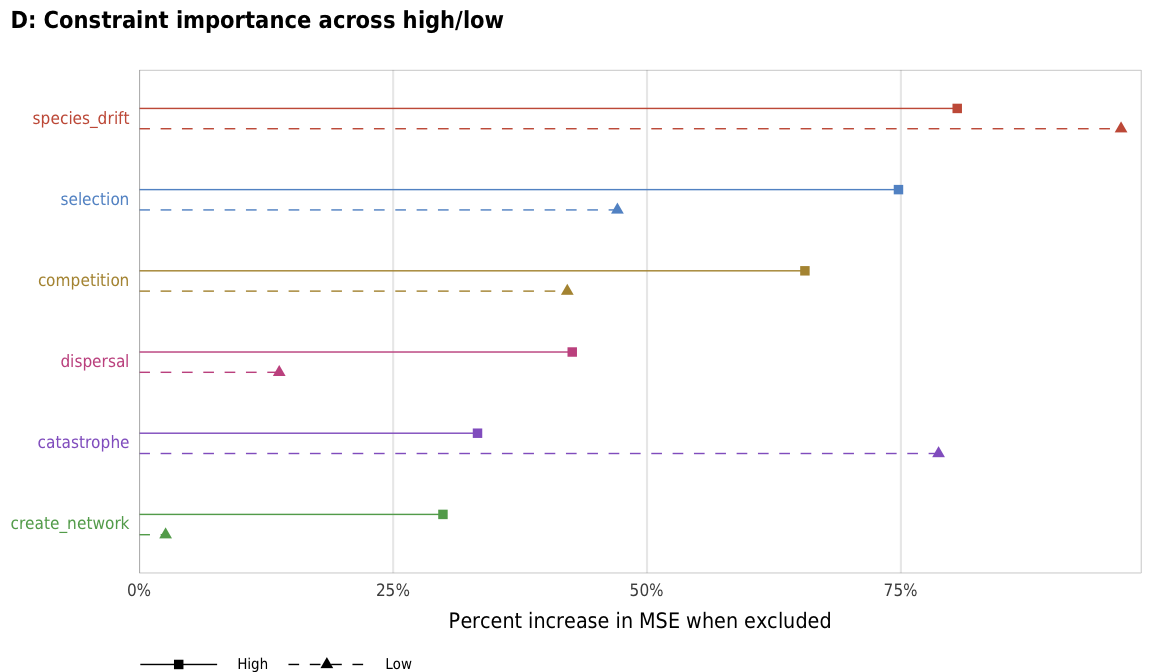
importance_evenness <- plot_evenness_importance_ls + plot_evenness_importance_hl

importance_evenness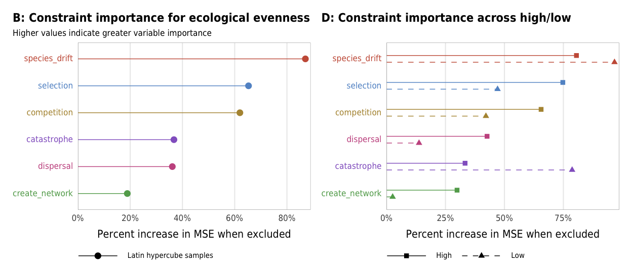
ggsave(importance_evenness, filename = here("analysis", "output", "evenness_importance.pdf"),
       width = params$fig_width2, height = params$fig_height, units = "in", device = cairo_pdf)
ggsave(importance_evenness, filename = here("analysis", "output", "evenness_importance.png"),
       width = params$fig_width2, height = params$fig_height, units = "in", type = "cairo", dpi = 300)
# ggsave(combined_fitness, filename = here("analysis", "output", "fitness_combined.eps"),
#        width = params$fig_width2, height = params$fig_height, units = "in", device = cairo_ps, fallback_resolution = 600)
plot_evenness_all <- mega_means_plot(constraint_combo_outcomes_ls, avg_evenness_t,
xlab = "Average ecological evenness",
title = "Average ecological evenness across combinations of constraints",
add_to_left = 0.08)
plot_evenness_all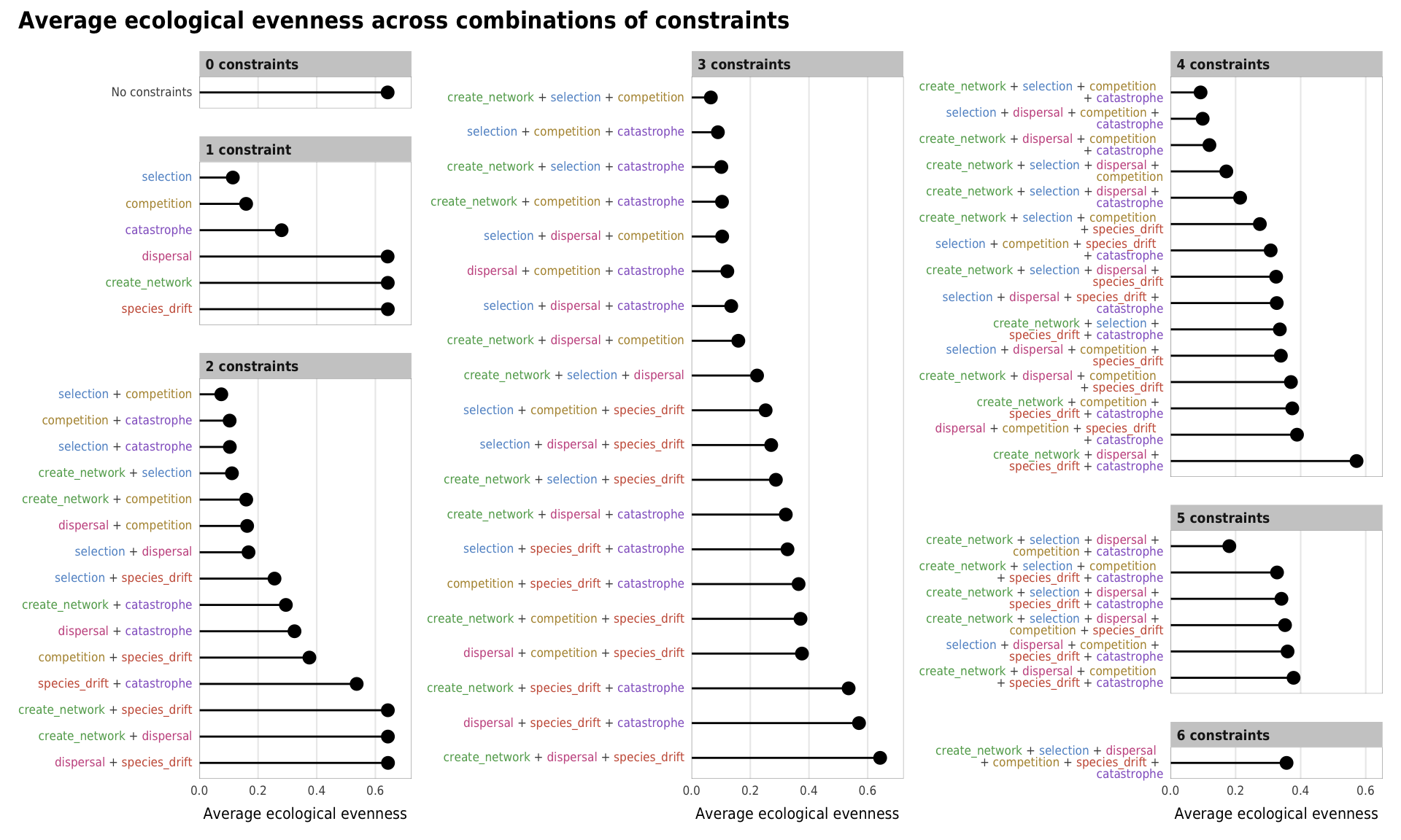
ggsave(plot_evenness_all, filename = here("analysis", "output", "evenness_means_all.pdf"),
       width = params$fig_width_big, height = params$fig_height_big, units = "in", device = cairo_pdf)
ggsave(plot_evenness_all, filename = here("analysis", "output", "evenness_means_all.png"),
       width = params$fig_width_big, height = params$fig_height_big, units = "in", type = "cairo", dpi = 300)
Figure 7: Landscape richness
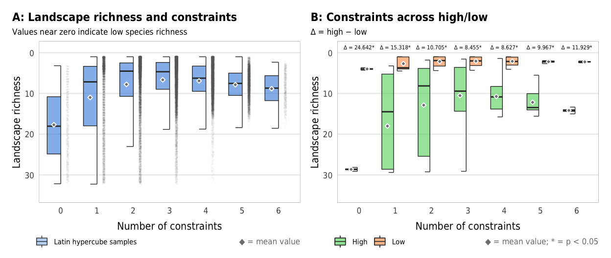
Fig 7. Effect of the number of constraints on species richness (A) Boxplots showing species richness across different numbers of constraints; (B) Percent increase in mean standard error in a random forest model when each constraint is removed; (C) Average species richness across all possible combinations of constraints
plot_richness_boxplot <- ggplot(sim_ls, aes(x = n_constraints_f, y = landscape_richness_mean)) +
  geom_half_point(size = 0.01, alpha = 0.01, side = "r", color = "grey50",
                  transformation_params = list(width = 0.25, height = 0, seed = 1234)) +
  geom_half_boxplot(aes(fill = "Latin hypercube samples"),
                    size = 0.25, side = "l", outlier.shape = NA, errorbar.draw = TRUE, alpha = 0.5) +
  stat_summary(geom = "point", fun = "mean",
               size = 1, pch = 23, fill = clrs$grey, color = "white",
               position = position_nudge(x = -0.19)) +
  scale_y_reverse() +
  scale_fill_manual(values = c("#0074D9"), name = NULL) +
  guides(fill = guide_legend(direction = "horizontal", override.aes = list(alpha = 0.3, size = 0.25))) +
  coord_cartesian(ylim = c(35, -1)) +
  labs(x = "Number of constraints",
       y = "Landscape richness",
       title = "A: Landscape richness and constraints",
       subtitle = "Values near zero indicate low species richness",
       caption = glue("<span style='color:{clrs$grey}'>◆</span> = mean value")) +
  theme_constraint() +
  theme(panel.grid.major.x = element_blank(),
        plot.caption = element_markdown(),
        plot.title.position = "plot",
        legend.position = c(0, 0),
        legend.justification = "left",
        legend.text = element_text(size = rel(0.7)),
        legend.box.margin = ggplot2::margin(l = -0.5, t = 4.15, unit = "lines"),
        legend.key.size = unit(0.75, "lines"))
plot_richness_boxplot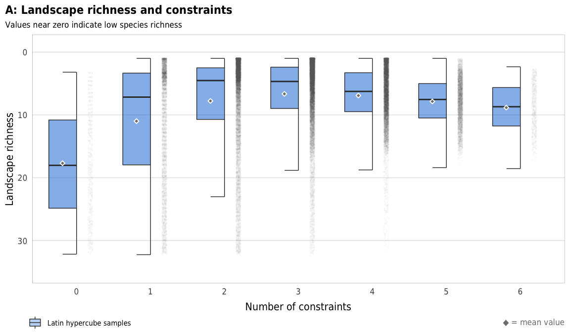
ggsave(plot_richness_boxplot, filename = here("analysis", "output", "richness_A.pdf"),
       width = params$fig_width, height = params$fig_height, units = "in", device = cairo_pdf)
ggsave(plot_richness_boxplot, filename = here("analysis", "output", "richness_A.png"),
       width = params$fig_width, height = params$fig_height, units = "in", type = "cairo", dpi = 300)
plot_richness_hl_diffs <- ggplot(mapping = aes(x = n_constraints_f, y = landscape_richness_mean, fill = repp)) +
geom_text(data = filter(diff_hl_outcomes_plot, outcome == "richness"),
aes(y = 0, label = nice_diff, fill = NULL),
family = "DejaVu Sans Condensed", fontface = "plain", size = 1.5, vjust = -0.85) +
geom_half_boxplot(data = sim_high,
size = 0.25, side = "l", outlier.shape = NA, errorbar.draw = TRUE,
nudge = 0.05, alpha = 0.5) +
geom_half_boxplot(data = sim_low,
size = 0.25, side = "r", outlier.shape = NA, errorbar.draw = TRUE,
nudge = 0.05, alpha = 0.5) +
stat_summary(data = sim_high, geom = "point", fun = "mean",
size = 1, pch = 23, fill = clrs$grey, color = "white",
position = position_nudge(x = -0.22)) +
stat_summary(data = sim_low, geom = "point", fun = "mean",
size = 1, pch = 23, fill = clrs$grey, color = "white",
position = position_nudge(x = 0.22)) +
scale_y_reverse() +
scale_fill_manual(values = c("#2ECC40", "#FF851B"), name = NULL) +
guides(fill = guide_legend(direction = "horizontal", override.aes = list(alpha = 0.3, size = 0.25))) +
coord_cartesian(ylim = c(35, -1)) +
labs(x = "Number of constraints",
y = "Landscape richness",
title = "B: Constraints across high/low",
subtitle = "∆ = high − low",
caption = glue("<span style='color:{clrs$grey}'>◆</span> = mean value; * = p < 0.05")) +
theme_constraint() +
theme(panel.grid.major.x = element_blank(),
plot.caption = element_markdown(),
plot.title.position = "plot",
legend.position = c(0, 0),
legend.justification = "left",
legend.text = element_text(size = rel(0.7)),
legend.box.margin = ggplot2::margin(l = -0.5, t = 4.15, unit = "lines"),
legend.key.size = unit(0.75, "lines"))
plot_richness_hl_diffs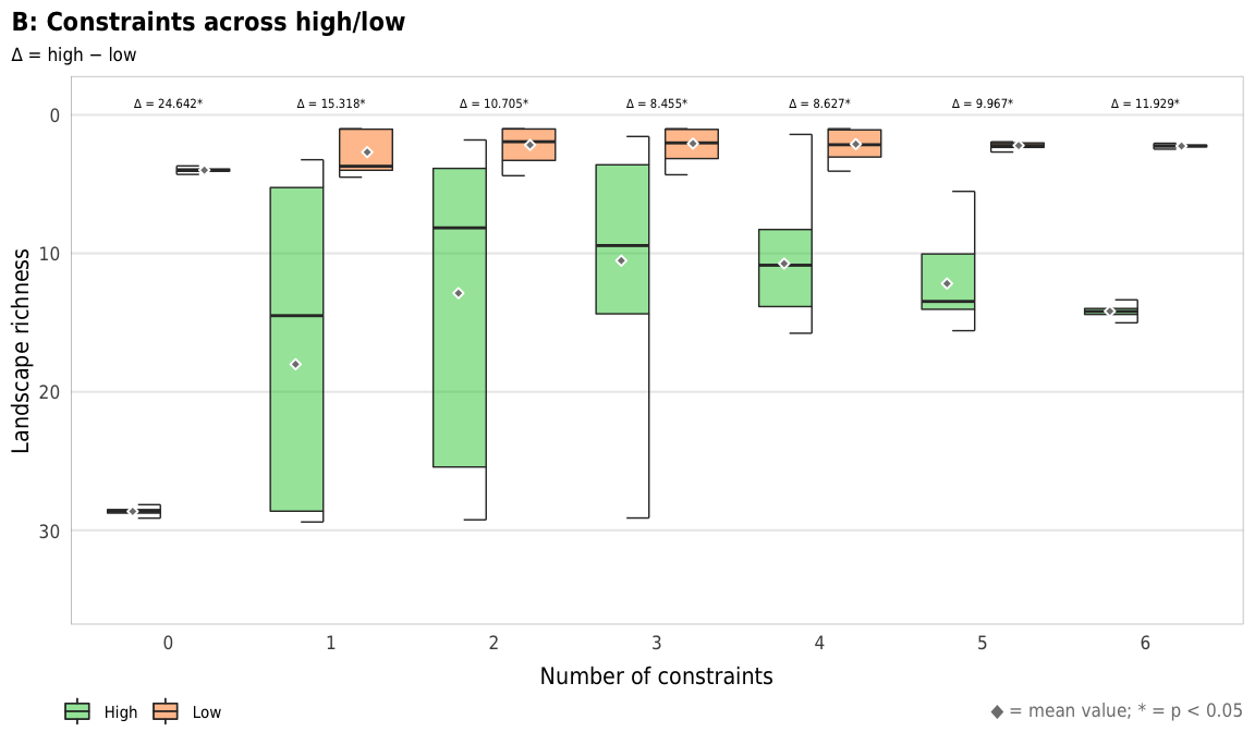
ggsave(combined_richness, filename = here("analysis", "output", "richness_boxplots.pdf"),
       width = params$fig_width2, height = params$fig_height, units = "in", device = cairo_pdf)
ggsave(combined_richness, filename = here("analysis", "output", "richness_boxplots.png"),
       width = params$fig_width2, height = params$fig_height, units = "in", type = "cairo", dpi = 300)
# ggsave(combined_richness, filename = here("analysis", "output", "richness_combined.tiff"),
#        width = params$fig_width2, height = params$fig_height, units = "in", type = "cairo", dpi = 600)
# ggsave(combined_richness, filename = here("analysis", "output", "richness_combined.eps"),
#        width = params$fig_width2, height = params$fig_height, units = "in", device = cairo_ps, fallback_resolution = 600)
# This takes a few minutes to run
set.seed(SEED)
forest_model_richness <-
randomForest(landscape_richness_mean ~
create_network + select + disperse +
compete + selectfor_d + catastrophe,
importance = TRUE,
data = drop_na(sim_ls, landscape_richness_mean))
forest_model_richness_low <-
randomForest(landscape_richness_mean ~
create_network + select + disperse +
compete + selectfor_d + catastrophe,
importance = TRUE,
data = filter(drop_na(sim_hl, landscape_richness_mean), repp == "Low"))
forest_model_richness_high <-
randomForest(landscape_richness_mean ~
create_network + select + disperse +
compete + selectfor_d + catastrophe,
importance = TRUE,
data = filter(drop_na(sim_hl, landscape_richness_mean), repp == "High"))richness_importance_ls <- importance(forest_model_richness, type = 1, scale = TRUE) %>%
data.frame() %>%
rownames_to_column(var = "constraint") %>%
arrange(desc(X.IncMSE)) %>%
mutate(constraint = recode(constraint,
`select` = "selection",
`compete` = "competition",
`disperse` = "dispersal",
`selectfor_d` = "species_drift")) %>%
color_constraints(constraint) %>%
mutate_at(vars(starts_with("constraint")), fct_inorder) %>%
mutate(X.IncMSE = X.IncMSE / 100)
plot_richness_importance_ls <- ggplot(richness_importance_ls,
aes(x = X.IncMSE, y = fct_rev(constraint_colored),
color = fct_rev(constraint), shape = "Latin hypercube samples")) +
geom_pointrangeh(aes(xmin = 0, xmax = X.IncMSE), size = 0.25) +
scale_x_continuous(labels = percent, expand = expansion(add = c(0, 0.02))) +
scale_color_manual(values = unlist(clrs), guide = FALSE) +
scale_shape_manual(values = c(19), name = NULL) +
guides(shape = guide_legend(direction = "horizontal",
override.aes = list(size = 0.25))) +
labs(x = "Percent increase in MSE when excluded", y = NULL,
title = "B: Constraint importance for landscape richness",
subtitle = "Higher values indicate greater variable importance",
caption = "") +
theme_constraint() +
theme(panel.grid.major.y = element_blank(),
axis.text.y = element_markdown(),
plot.title.position = "plot",
legend.position = c(0, 0),
legend.justification = "left",
legend.text = element_markdown(size = rel(0.7)),
legend.box.margin = ggplot2::margin(l = -0.5, t = 4.75, unit = "lines"),
legend.key.width = unit(2.5, "lines"),
legend.key.size = unit(0.95, "lines"))
plot_richness_importance_ls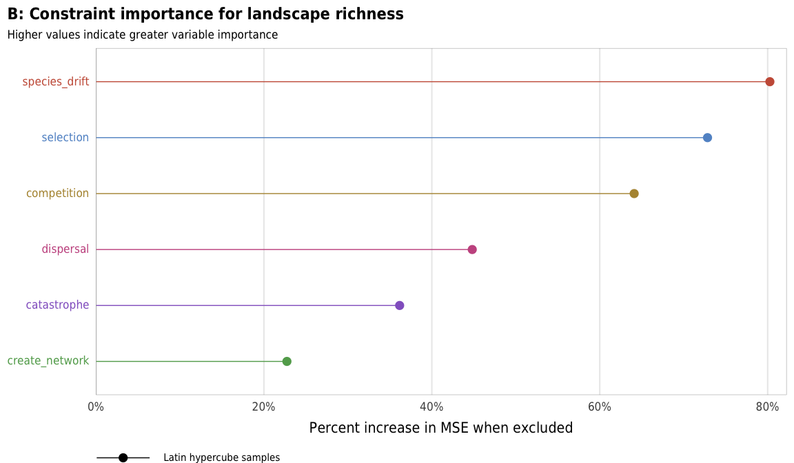
ggsave(plot_richness_importance_ls, filename = here("analysis", "output", "richness_B.pdf"),
       width = params$fig_width, height = params$fig_height, units = "in", device = cairo_pdf)
ggsave(plot_richness_importance_ls, filename = here("analysis", "output", "richness_B.png"),
       width = params$fig_width, height = params$fig_height, units = "in", type = "cairo", dpi = 300)
richness_importance_low <- importance(forest_model_richness_low, type = 1, scale = TRUE) %>%
data.frame() %>%
rownames_to_column(var = "constraint") %>%
mutate(repp = "Low")
richness_importance_high <- importance(forest_model_richness_high, type = 1, scale = TRUE) %>%
data.frame() %>%
rownames_to_column(var = "constraint") %>%
mutate(repp = "High")
richness_importance_hl <- bind_rows(richness_importance_low,
richness_importance_high) %>%
mutate(repp = factor(repp, levels = c("Low", "High"), ordered = TRUE)) %>%
arrange(desc(repp), desc(X.IncMSE)) %>%
mutate(constraint = recode(constraint,
`select` = "selection",
`compete` = "competition",
`disperse` = "dispersal",
`selectfor_d` = "species_drift")) %>%
color_constraints(constraint) %>%
mutate_at(vars(starts_with("constraint")), fct_inorder) %>%
mutate(X.IncMSE = X.IncMSE / 100)
plot_richness_importance_hl <- ggplot(richness_importance_hl,
aes(x = X.IncMSE, y = fct_rev(constraint_colored),
color = fct_rev(constraint),
linetype = repp, shape = repp)) +
geom_pointrangeh(aes(xmin = 0, xmax = X.IncMSE),
position = position_dodgev(height = 0.5), size = 0.25) +
scale_x_continuous(labels = percent, expand = expansion(add = c(0, 0.02))) +
scale_color_manual(values = unlist(clrs), guide = FALSE) +
scale_linetype_manual(values = c("dashed", "solid"), name = NULL) +
scale_shape_manual(values = c(17, 15), name = NULL) +
guides(linetype = guide_legend(direction = "horizontal", reverse = TRUE),
shape = guide_legend(direction = "horizontal", override.aes = list(size = 0.25),
reverse = TRUE)) +
labs(x = "Percent increase in MSE when excluded", y = NULL,
title = "D: Constraint importance across high/low",
subtitle = "",
caption = "") +
theme_constraint() +
theme(panel.grid.major.y = element_blank(),
axis.text.y = element_markdown(),
plot.title.position = "plot",
legend.position = c(0, 0),
legend.justification = "left",
legend.text = element_markdown(size = rel(0.7)),
legend.box.margin = ggplot2::margin(l = -0.5, t = 4.75, unit = "lines"),
legend.key.width = unit(2.5, "lines"),
legend.key.size = unit(0.95, "lines"))
plot_richness_importance_hl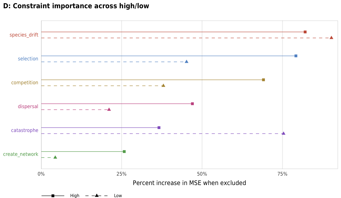
importance_richness <- plot_richness_importance_ls + plot_richness_importance_hl

importance_richness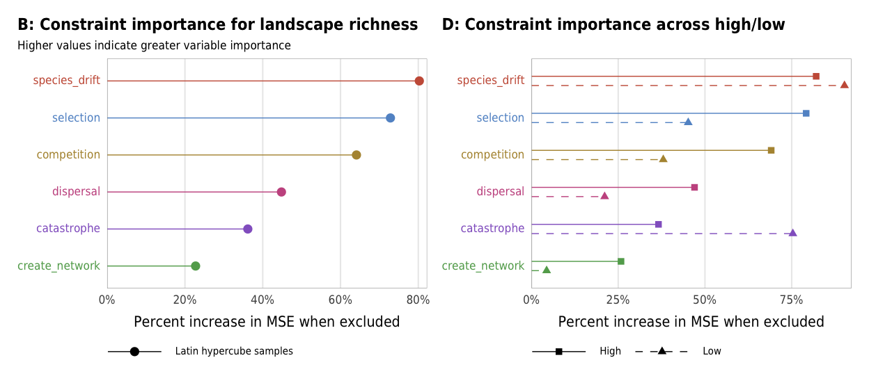
ggsave(importance_richness, filename = here("analysis", "output", "richness_importance.pdf"),
       width = params$fig_width2, height = params$fig_height, units = "in", device = cairo_pdf)
ggsave(importance_richness, filename = here("analysis", "output", "richness_importance.png"),
       width = params$fig_width2, height = params$fig_height, units = "in", type = "cairo", dpi = 300)
# ggsave(combined_fitness, filename = here("analysis", "output", "fitness_combined.tiff"),
#        width = params$fig_width2, height = params$fig_height, units = "in", type = "cairo", dpi = 600)
# ggsave(combined_fitness, filename = here("analysis", "output", "fitness_combined.eps"),
#        width = params$fig_width2, height = params$fig_height, units = "in", device = cairo_ps, fallback_resolution = 600)
plot_richness_all <- mega_means_plot(constraint_combo_outcomes_ls, landscape_richness_mean,
xlab = "Average landscape richness",
title = "Average landscape richness across combinations of constraints",
add_to_left = 1)
plot_richness_all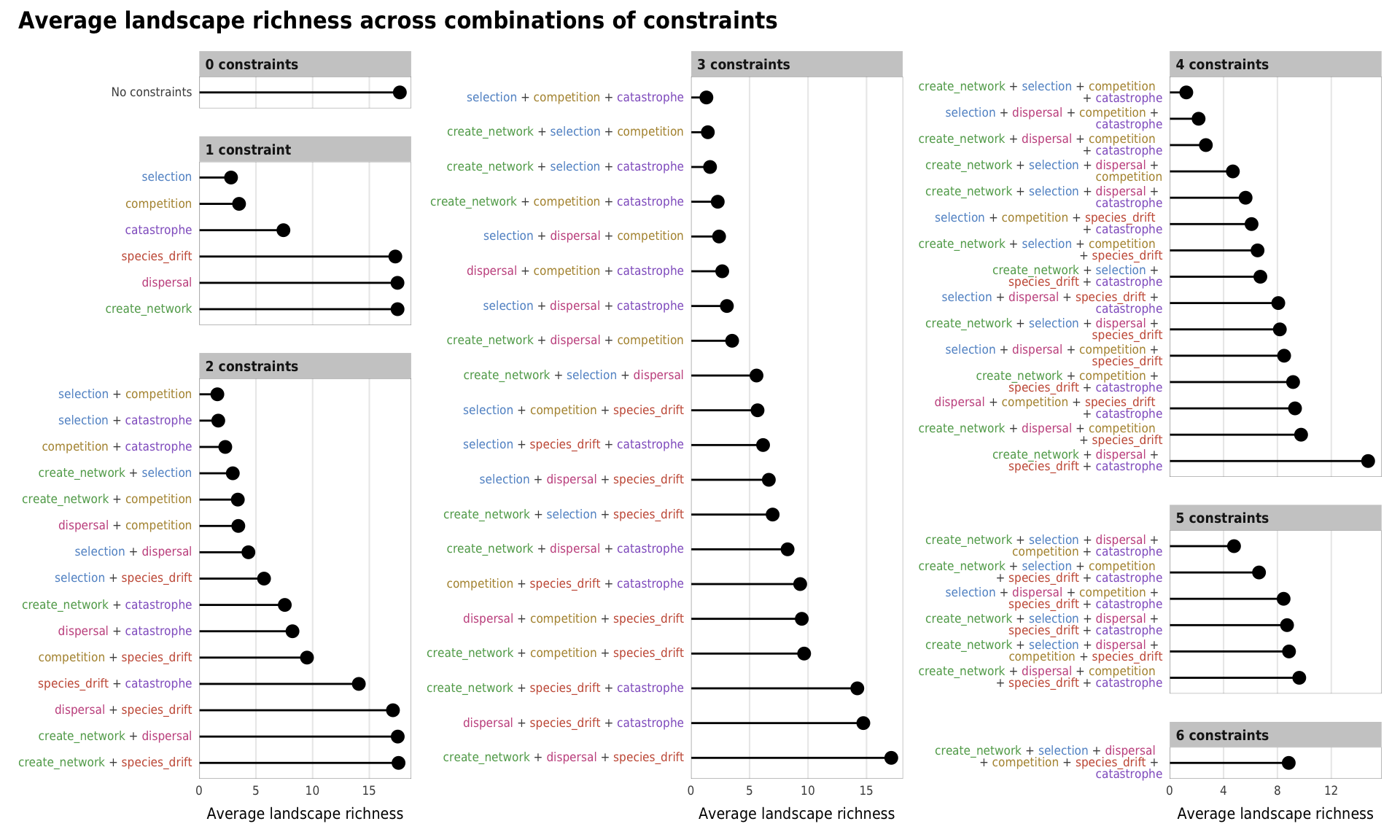
ggsave(plot_richness_all, filename = here("analysis", "output", "richness_means_all.pdf"),
       width = params$fig_width_big, height = params$fig_height_big, units = "in", device = cairo_pdf)
ggsave(plot_richness_all, filename = here("analysis", "output", "richness_means_all.png"),
       width = params$fig_width_big, height = params$fig_height_big, units = "in", type = "cairo", dpi = 300)
Figure 8: Difference in turnover
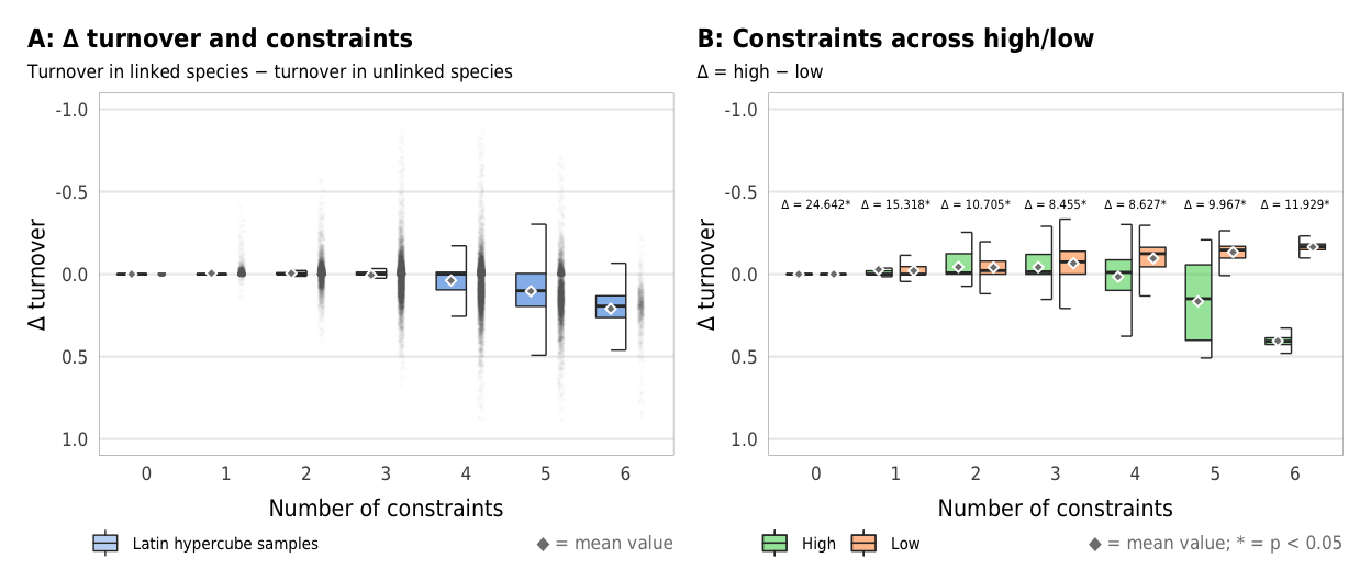
Fig 8. Effect of the number of constraints on the difference between turnover in linked and unlinked species (A) Boxplots showing difference between turnover in linked and unlinked species across different numbers of constraints; (B) Percent increase in mean standard error in a random forest model when each constraint is removed; (C) Average difference across all possible combinations of constraints
plot_turnover_boxplot <- ggplot(sim_ls, aes(x = n_constraints_f, y = turnover_diff)) +
  geom_half_point(size = 0.01, alpha = 0.01, side = "r", color = "grey50",
                  transformation_params = list(width = 0.25, height = 0, seed = 1234)) +
  geom_half_boxplot(aes(fill = "Latin hypercube samples"),
                    size = 0.25, side = "l", outlier.shape = NA, errorbar.draw = TRUE, alpha = 0.5) +
  stat_summary(geom = "point", fun = "mean",
               size = 1, pch = 23, fill = clrs$grey, color = "white",
               position = position_nudge(x = -0.19)) +
  scale_y_reverse() +
  scale_fill_manual(values = c("#0074D9"), name = NULL) +
  guides(fill = guide_legend(direction = "horizontal", override.aes = list(alpha = 0.3, size = 0.25))) +
  coord_cartesian(ylim = c(1, -1)) +
  labs(x = "Number of constraints",
       y = "∆ turnover",
       title = "A: ∆ turnover and constraints",
       subtitle = "Turnover in linked species − turnover in unlinked species",
       caption = glue("<span style='color:{clrs$grey}'>◆</span> = mean value")) +
  theme_constraint() +
  theme(panel.grid.major.x = element_blank(),
        plot.caption = element_markdown(),
        plot.title.position = "plot",
        legend.position = c(0, 0),
        legend.justification = "left",
        legend.text = element_text(size = rel(0.7)),
        legend.box.margin = ggplot2::margin(l = -0.5, t = 4.15, unit = "lines"),
        legend.key.size = unit(0.75, "lines"))
plot_turnover_boxplot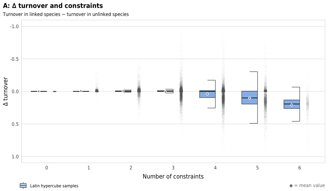
ggsave(plot_turnover_boxplot, filename = here("analysis", "output", "turnover_A.pdf"),
       width = params$fig_width, height = params$fig_height, units = "in", device = cairo_pdf)
ggsave(plot_turnover_boxplot, filename = here("analysis", "output", "turnover_A.png"),
       width = params$fig_width, height = params$fig_height, units = "in", type = "cairo", dpi = 300)
plot_turnover_hl_diffs <- ggplot(mapping = aes(x = n_constraints_f, y = turnover_diff, fill = repp)) +
geom_text(data = filter(diff_hl_outcomes_plot, outcome == "richness"),
aes(y = -0.35, label = nice_diff, fill = NULL),
family = "DejaVu Sans Condensed", fontface = "plain", size = 1.5, vjust = -0.85) +
geom_half_boxplot(data = sim_high,
size = 0.25, side = "l", outlier.shape = NA, errorbar.draw = TRUE,
nudge = 0.05, alpha = 0.5) +
geom_half_boxplot(data = sim_low,
size = 0.25, side = "r", outlier.shape = NA, errorbar.draw = TRUE,
nudge = 0.05, alpha = 0.5) +
stat_summary(data = sim_high, geom = "point", fun = "mean",
size = 1, pch = 23, fill = clrs$grey, color = "white",
position = position_nudge(x = -0.22)) +
stat_summary(data = sim_low, geom = "point", fun = "mean",
size = 1, pch = 23, fill = clrs$grey, color = "white",
position = position_nudge(x = 0.22)) +
scale_y_reverse() +
scale_fill_manual(values = c("#2ECC40", "#FF851B"), name = NULL) +
guides(fill = guide_legend(direction = "horizontal", override.aes = list(alpha = 0.3, size = 0.25))) +
coord_cartesian(ylim = c(1, -1)) +
labs(x = "Number of constraints",
y = "∆ turnover",
title = "B: Constraints across high/low",
subtitle = "∆ = high − low",
caption = glue("<span style='color:{clrs$grey}'>◆</span> = mean value; * = p < 0.05")) +
theme_constraint() +
theme(panel.grid.major.x = element_blank(),
plot.caption = element_markdown(),
plot.title.position = "plot",
legend.position = c(0, 0),
legend.justification = "left",
legend.text = element_text(size = rel(0.7)),
legend.box.margin = ggplot2::margin(l = -0.5, t = 4.15, unit = "lines"),
legend.key.size = unit(0.75, "lines"))
plot_turnover_hl_diffs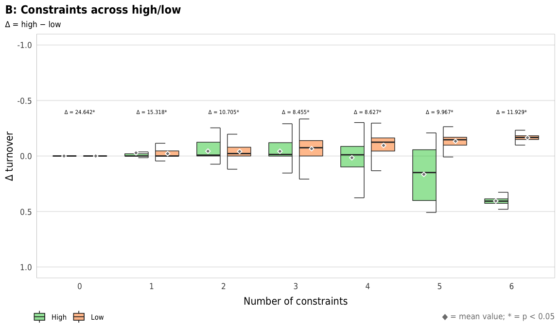
ggsave(combined_turnover, filename = here("analysis", "output", "turnover_boxplots.pdf"),
       width = params$fig_width2, height = params$fig_height, units = "in", device = cairo_pdf)
ggsave(combined_turnover, filename = here("analysis", "output", "turnover_boxplots.png"),
       width = params$fig_width2, height = params$fig_height, units = "in", type = "cairo", dpi = 300)
# ggsave(combined_turnover, filename = here("analysis", "output", "turnover_combined.tiff"),
#        width = params$fig_width2, height = params$fig_height, units = "in", type = "cairo", dpi = 600)
# ggsave(combined_turnover, filename = here("analysis", "output", "turnover_combined.eps"),
#        width = params$fig_width2, height = params$fig_height, units = "in", device = cairo_ps, fallback_resolution = 600)
# This takes a few minutes to run
set.seed(SEED)
forest_model_turnover <-
randomForest(turnover_diff ~
create_network + select + disperse +
compete + selectfor_d + catastrophe,
importance = TRUE,
data = drop_na(sim_ls, turnover_diff))
forest_model_turnover_low <-
randomForest(turnover_diff ~
create_network + select + disperse +
compete + selectfor_d + catastrophe,
importance = TRUE,
data = filter(drop_na(sim_hl, turnover_diff), repp == "Low"))
forest_model_turnover_high <-
randomForest(turnover_diff ~
create_network + select + disperse +
compete + selectfor_d + catastrophe,
importance = TRUE,
data = filter(drop_na(sim_hl, turnover_diff), repp == "High"))turnover_importance_ls <- importance(forest_model_turnover, type = 1, scale = TRUE) %>%
data.frame() %>%
rownames_to_column(var = "constraint") %>%
arrange(desc(X.IncMSE)) %>%
mutate(constraint = recode(constraint,
`select` = "selection",
`compete` = "competition",
`disperse` = "dispersal",
`selectfor_d` = "species_drift")) %>%
color_constraints(constraint) %>%
mutate_at(vars(starts_with("constraint")), fct_inorder) %>%
mutate(X.IncMSE = X.IncMSE / 100)
plot_turnover_importance_ls <- ggplot(turnover_importance_ls,
aes(x = X.IncMSE, y = fct_rev(constraint_colored),
color = fct_rev(constraint),
shape = "Latin hypercube samples")) +
geom_pointrangeh(aes(xmin = 0, xmax = X.IncMSE), size = 0.25) +
scale_x_continuous(labels = percent, expand = expansion(add = c(0, 0.02))) +
scale_color_manual(values = unlist(clrs), guide = FALSE) +
scale_shape_manual(values = c(19), name = NULL) +
guides(shape = guide_legend(direction = "horizontal",
override.aes = list(size = 0.25))) +
labs(x = "Percent increase in MSE when excluded", y = NULL,
title = "B: Constraint importance for ∆ species turnover",
subtitle = "Higher values indicate greater variable importance",
caption = "") +
theme_constraint() +
theme(panel.grid.major.y = element_blank(),
axis.text.y = element_markdown(),
plot.title.position = "plot",
legend.position = c(0, 0),
legend.justification = "left",
legend.text = element_markdown(size = rel(0.7)),
legend.box.margin = ggplot2::margin(l = -0.5, t = 4.75, unit = "lines"),
legend.key.width = unit(2.5, "lines"),
legend.key.size = unit(0.95, "lines"))
plot_turnover_importance_ls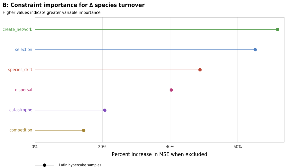
ggsave(plot_turnover_importance_ls, filename = here("analysis", "output", "turnover_B.pdf"),
       width = params$fig_width, height = params$fig_height, units = "in", device = cairo_pdf)
ggsave(plot_turnover_importance_ls, filename = here("analysis", "output", "turnover_B.png"),
       width = params$fig_width, height = params$fig_height, units = "in", type = "cairo", dpi = 300)
turnover_importance_low <- importance(forest_model_turnover_low, type = 1, scale = TRUE) %>%
data.frame() %>%
rownames_to_column(var = "constraint") %>%
mutate(repp = "Low")
turnover_importance_high <- importance(forest_model_turnover_high, type = 1, scale = TRUE) %>%
data.frame() %>%
rownames_to_column(var = "constraint") %>%
mutate(repp = "High")
turnover_importance_hl <- bind_rows(turnover_importance_low,
turnover_importance_high) %>%
mutate(repp = factor(repp, levels = c("Low", "High"), ordered = TRUE)) %>%
arrange(desc(repp), desc(X.IncMSE)) %>%
mutate(constraint = recode(constraint,
`select` = "selection",
`compete` = "competition",
`disperse` = "dispersal",
`selectfor_d` = "species_drift")) %>%
color_constraints(constraint) %>%
mutate_at(vars(starts_with("constraint")), fct_inorder) %>%
mutate(X.IncMSE = X.IncMSE / 100)
plot_turnover_importance_hl <- ggplot(turnover_importance_hl,
aes(x = X.IncMSE, y = fct_rev(constraint_colored),
color = fct_rev(constraint),
linetype = repp, shape = repp)) +
geom_pointrangeh(aes(xmin = 0, xmax = X.IncMSE),
position = position_dodgev(height = 0.5), size = 0.25) +
scale_x_continuous(labels = percent, expand = expansion(add = c(0, 0.02))) +
scale_color_manual(values = unlist(clrs), guide = FALSE) +
scale_linetype_manual(values = c("dashed", "solid"), name = NULL) +
scale_shape_manual(values = c(17, 15), name = NULL) +
guides(linetype = guide_legend(direction = "horizontal", reverse = TRUE),
shape = guide_legend(direction = "horizontal", override.aes = list(size = 0.25),
reverse = TRUE)) +
labs(x = "Percent increase in MSE when excluded", y = NULL,
title = "D: Constraint importance across high/low",
subtitle = "",
caption = "") +
theme_constraint() +
theme(panel.grid.major.y = element_blank(),
axis.text.y = element_markdown(),
plot.title.position = "plot",
legend.position = c(0, 0),
legend.justification = "left",
legend.text = element_markdown(size = rel(0.7)),
legend.box.margin = ggplot2::margin(l = -0.5, t = 4.75, unit = "lines"),
legend.key.width = unit(2.5, "lines"),
legend.key.size = unit(0.95, "lines"))
plot_turnover_importance_hl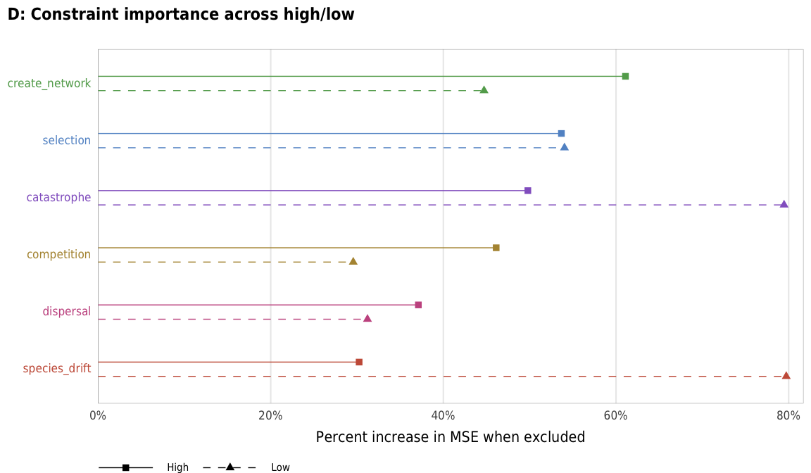
importance_turnover <- plot_turnover_importance_ls + plot_turnover_importance_hl

importance_turnover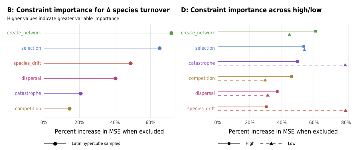
ggsave(importance_turnover, filename = here("analysis", "output", "turnover_importance.pdf"),
       width = params$fig_width2, height = params$fig_height, units = "in", device = cairo_pdf)
ggsave(importance_turnover, filename = here("analysis", "output", "turnover_importance.png"),
       width = params$fig_width2, height = params$fig_height, units = "in", type = "cairo", dpi = 300)
# ggsave(combined_fitness, filename = here("analysis", "output", "fitness_combined.tiff"),
#        width = params$fig_width2, height = params$fig_height, units = "in", type = "cairo", dpi = 600)
# ggsave(combined_fitness, filename = here("analysis", "output", "fitness_combined.eps"),
#        width = params$fig_width2, height = params$fig_height, units = "in", device = cairo_ps, fallback_resolution = 600)
plot_turnover_all <- mega_means_plot(constraint_combo_outcomes_ls, turnover_diff,
xlab = "Average ∆ turnover",
title = "Average ∆ in turnover (linked species − unlinked species) across combinations of constraints",
add_to_right = 0.02, add_to_left = 0.02, xlim = c(-0.1, 0.3))
plot_turnover_all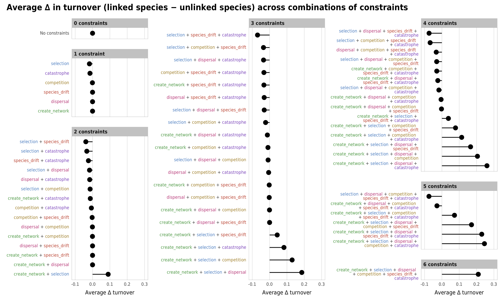
ggsave(plot_turnover_all, filename = here("analysis", "output", "turnover_means_all.pdf"),
       width = params$fig_width_big, height = params$fig_height_big, units = "in", device = cairo_pdf)
ggsave(plot_turnover_all, filename = here("analysis", "output", "turnover_means_all.png"),
       width = params$fig_width_big, height = params$fig_height_big, units = "in", type = "cairo", dpi = 300)
Figure 9: Landscape variation
Fig 9. Overall landscape variation in species richness
plot_variation_boxplot <- ggplot(sim_ls, aes(x = n_constraints_f, y = landscape_species_number_var)) +
  geom_half_point(size = 0.01, alpha = 0.01, side = "r", color = "grey50",
                  transformation_params = list(width = 0.25, height = 0, seed = 1234)) +
  geom_half_boxplot(aes(fill = "Latin hypercube samples"),
                    size = 0.25, side = "l", outlier.shape = NA, errorbar.draw = TRUE, alpha = 0.5) +
  stat_summary(geom = "point", fun = "mean",
               size = 1, pch = 23, fill = clrs$grey, color = "white",
               position = position_nudge(x = -0.19)) +
  # scale_y_reverse() +
  scale_fill_manual(values = c("#0074D9"), name = NULL) +
  guides(fill = guide_legend(direction = "horizontal", override.aes = list(alpha = 0.3, size = 0.25))) +
  coord_cartesian(ylim = c(0, 300)) +
  labs(x = "Number of constraints",
       y = "Landscape variation in species richness",
       title = "A: Landscape variation in species richness",
       # subtitle = "Values near zero indicate high variation",
       caption = glue("<span style='color:{clrs$grey}'>◆</span> = mean value")) +
  theme_constraint() +
  theme(panel.grid.major.x = element_blank(),
        plot.caption = element_markdown(),
        plot.title.position = "plot",
        legend.position = c(0, 0),
        legend.justification = "left",
        legend.text = element_text(size = rel(0.7)),
        legend.box.margin = ggplot2::margin(l = -0.5, t = 4.15, unit = "lines"),
        legend.key.size = unit(0.75, "lines"))
plot_variation_boxplot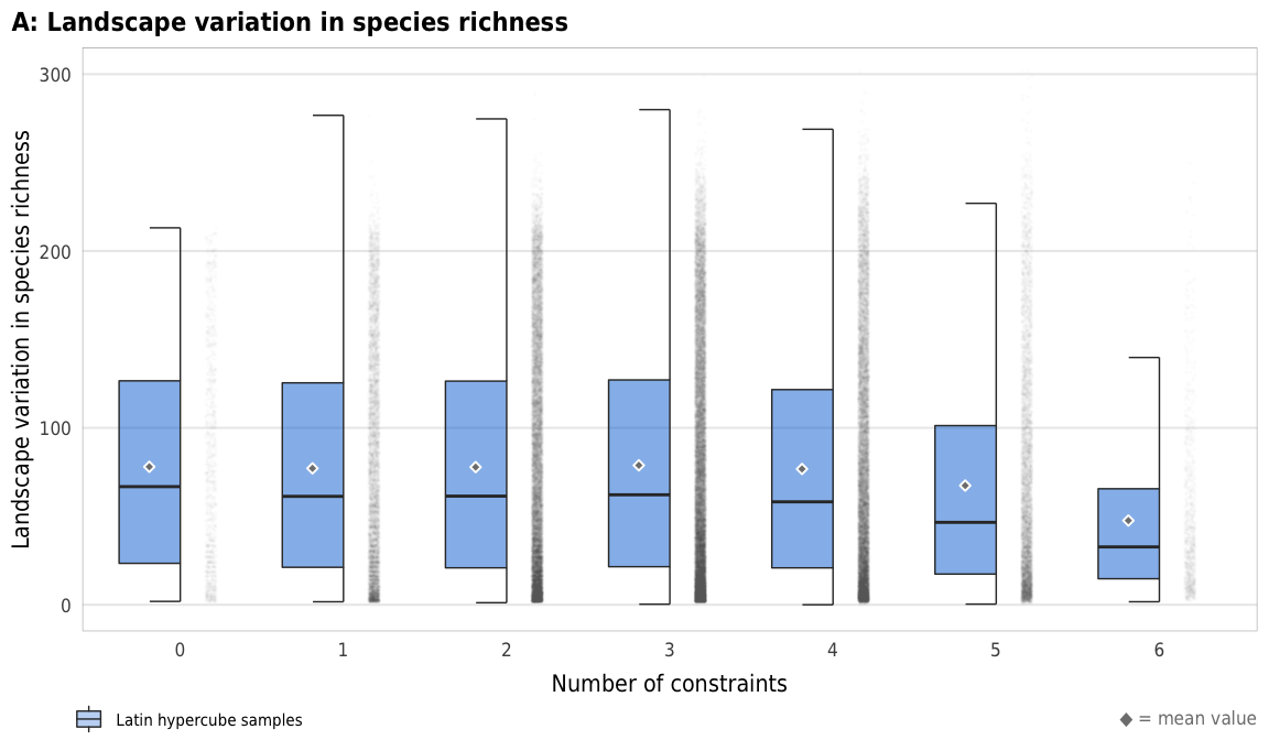
ggsave(plot_variation_boxplot, filename = here("analysis", "output", "landscape_species.pdf"),
       width = params$fig_width, height = params$fig_height, units = "in", device = cairo_pdf)
ggsave(plot_variation_boxplot, filename = here("analysis", "output", "landscape_species.png"),
       width = params$fig_width, height = params$fig_height, units = "in", type = "cairo", dpi = 300)
Original computing environment
## # http://dirk.eddelbuettel.com/blog/2017/11/27/#011_faster_package_installation_one
## VER=
## CCACHE=ccache
## CC=$(CCACHE) gcc$(VER)
## CXX=$(CCACHE) g++$(VER)
## CXX11=$(CCACHE) g++$(VER)
## CXX14=$(CCACHE) g++$(VER)
## FC=$(CCACHE) gfortran$(VER)
## F77=$(CCACHE) gfortran$(VER)
##
## CXX14FLAGS=-O3 -march=native -mtune=native -fPIC## ─ Session info ───────────────────────────────────────────────────────────────
## setting value
## version R version 4.0.2 (2020-06-22)
## os macOS Catalina 10.15.6
## system x86_64, darwin17.0
## ui X11
## language (EN)
## collate en_US.UTF-8
## ctype en_US.UTF-8
## tz America/New_York
## date 2020-09-12
##
## ─ Packages ───────────────────────────────────────────────────────────────────
## package * version date lib source
## assertthat 0.2.1 2019-03-21 [1] CRAN (R 4.0.0)
## backports 1.1.9 2020-08-24 [1] CRAN (R 4.0.2)
## base64enc 0.1-3 2015-07-28 [1] CRAN (R 4.0.0)
## blob 1.2.1 2020-01-20 [1] CRAN (R 4.0.0)
## broom * 0.7.0 2020-07-09 [1] CRAN (R 4.0.2)
## callr 3.4.3 2020-03-28 [1] CRAN (R 4.0.0)
## cellranger 1.1.0 2016-07-27 [1] CRAN (R 4.0.0)
## cli 2.0.2 2020-02-28 [1] CRAN (R 4.0.0)
## colorspace 1.4-1 2019-03-18 [1] CRAN (R 4.0.0)
## crayon 1.3.4 2017-09-16 [1] CRAN (R 4.0.0)
## curl 4.3 2019-12-02 [1] CRAN (R 4.0.0)
## DBI 1.1.0 2019-12-15 [1] CRAN (R 4.0.0)
## dbplyr 1.4.4 2020-05-27 [1] CRAN (R 4.0.2)
## desc 1.2.0 2018-05-01 [1] CRAN (R 4.0.0)
## devtools 2.3.1 2020-07-21 [1] CRAN (R 4.0.2)
## digest 0.6.25 2020-02-23 [1] CRAN (R 4.0.0)
## dplyr * 1.0.2 2020-08-18 [1] CRAN (R 4.0.2)
## ellipsis 0.3.1 2020-05-15 [1] CRAN (R 4.0.0)
## evaluate 0.14 2019-05-28 [1] CRAN (R 4.0.0)
## fansi 0.4.1 2020-01-08 [1] CRAN (R 4.0.0)
## farver 2.0.3 2020-01-16 [1] CRAN (R 4.0.0)
## forcats * 0.5.0 2020-03-01 [1] CRAN (R 4.0.0)
## fs 1.5.0 2020-07-31 [1] CRAN (R 4.0.2)
## generics 0.0.2 2018-11-29 [1] CRAN (R 4.0.0)
## ggforce * 0.3.2 2020-06-23 [1] CRAN (R 4.0.2)
## gghalves * 0.1.0 2020-03-28 [1] CRAN (R 4.0.0)
## ggplot2 * 3.3.2 2020-06-19 [1] CRAN (R 4.0.2)
## ggstance * 0.3.4 2020-04-02 [1] CRAN (R 4.0.0)
## ggtext * 0.1.0 2020-05-20 [1] Github (wilkelab/ggtext@e978034)
## glue * 1.4.2 2020-08-27 [1] CRAN (R 4.0.2)
## gridtext 0.1.1 2020-02-24 [1] CRAN (R 4.0.0)
## gtable 0.3.0 2019-03-25 [1] CRAN (R 4.0.0)
## haven 2.3.1 2020-06-01 [1] CRAN (R 4.0.2)
## here * 0.1 2017-05-28 [1] CRAN (R 4.0.0)
## hms 0.5.3 2020-01-08 [1] CRAN (R 4.0.0)
## htmltools 0.5.0 2020-06-16 [1] CRAN (R 4.0.0)
## httr 1.4.2 2020-07-20 [1] CRAN (R 4.0.2)
## jsonlite 1.7.0 2020-06-25 [1] CRAN (R 4.0.2)
## knitr 1.29 2020-06-23 [1] CRAN (R 4.0.2)
## labeling 0.3 2014-08-23 [1] CRAN (R 4.0.0)
## lifecycle 0.2.0 2020-03-06 [1] CRAN (R 4.0.0)
## lubridate 1.7.9 2020-06-08 [1] CRAN (R 4.0.2)
## magrittr 1.5 2014-11-22 [1] CRAN (R 4.0.0)
## markdown 1.1 2019-08-07 [1] CRAN (R 4.0.0)
## MASS 7.3-52 2020-08-18 [1] CRAN (R 4.0.2)
## memoise 1.1.0 2017-04-21 [1] CRAN (R 4.0.0)
## modelr 0.1.8 2020-05-19 [1] CRAN (R 4.0.2)
## munsell 0.5.0 2018-06-12 [1] CRAN (R 4.0.0)
## pander * 0.6.3 2018-11-06 [1] CRAN (R 4.0.0)
## patchwork * 1.0.1 2020-06-22 [1] CRAN (R 4.0.2)
## pillar 1.4.6 2020-07-10 [1] CRAN (R 4.0.2)
## pkgbuild 1.1.0 2020-07-13 [1] CRAN (R 4.0.2)
## pkgconfig 2.0.3 2019-09-22 [1] CRAN (R 4.0.0)
## pkgload 1.1.0 2020-05-29 [1] CRAN (R 4.0.2)
## pluralize * 0.2.0 2020-06-09 [1] CRAN (R 4.0.2)
## plyr 1.8.6 2020-03-03 [1] CRAN (R 4.0.0)
## polyclip 1.10-0 2019-03-14 [1] CRAN (R 4.0.0)
## prettyunits 1.1.1 2020-01-24 [1] CRAN (R 4.0.0)
## processx 3.4.3 2020-07-05 [1] CRAN (R 4.0.0)
## ps 1.3.4 2020-08-11 [1] CRAN (R 4.0.2)
## purrr * 0.3.4 2020-04-17 [1] CRAN (R 4.0.0)
## R6 2.4.1 2019-11-12 [1] CRAN (R 4.0.0)
## randomForest * 4.6-14 2018-03-25 [1] CRAN (R 4.0.2)
## Rcpp 1.0.5 2020-07-06 [1] CRAN (R 4.0.2)
## readr * 1.3.1 2018-12-21 [1] CRAN (R 4.0.0)
## readxl 1.3.1 2019-03-13 [1] CRAN (R 4.0.0)
## remotes 2.2.0 2020-07-21 [1] CRAN (R 4.0.2)
## reprex 0.3.0 2019-05-16 [1] CRAN (R 4.0.0)
## rlang 0.4.7 2020-07-09 [1] CRAN (R 4.0.2)
## rmarkdown 2.3 2020-06-18 [1] CRAN (R 4.0.2)
## rprojroot 1.3-2 2018-01-03 [1] CRAN (R 4.0.0)
## rstudioapi 0.11 2020-02-07 [1] CRAN (R 4.0.0)
## rvest 0.3.6 2020-07-25 [1] CRAN (R 4.0.2)
## scales * 1.1.1 2020-05-11 [1] CRAN (R 4.0.0)
## sessioninfo 1.1.1 2018-11-05 [1] CRAN (R 4.0.0)
## stringi 1.4.6 2020-02-17 [1] CRAN (R 4.0.0)
## stringr * 1.4.0 2019-02-10 [1] CRAN (R 4.0.0)
## testthat 2.3.2 2020-03-02 [1] CRAN (R 4.0.0)
## tibble * 3.0.3 2020-07-10 [1] CRAN (R 4.0.2)
## tidyr * 1.1.2 2020-08-27 [1] CRAN (R 4.0.2)
## tidyselect 1.1.0 2020-05-11 [1] CRAN (R 4.0.0)
## tidyverse * 1.3.0 2019-11-21 [1] CRAN (R 4.0.0)
## titanic * 0.1.0 2015-08-31 [1] CRAN (R 4.0.2)
## tweenr 1.0.1 2018-12-14 [1] CRAN (R 4.0.0)
## usethis 1.6.1 2020-04-29 [1] CRAN (R 4.0.0)
## V8 3.2.0 2020-06-19 [1] CRAN (R 4.0.2)
## vctrs 0.3.4 2020-08-29 [1] CRAN (R 4.0.2)
## withr 2.2.0 2020-04-20 [1] CRAN (R 4.0.0)
## xfun 0.16 2020-07-24 [1] CRAN (R 4.0.2)
## xml2 1.3.2 2020-04-23 [1] CRAN (R 4.0.0)
## yaml 2.2.1 2020-02-01 [1] CRAN (R 4.0.0)
##
## [1] /Library/Frameworks/R.framework/Versions/4.0/Resources/library