Theoretical and empirical estimands
TODO: We can’t just say (in words or in math) that we want to know the effect of crackdowns on aid. We need to incorporate the within or between effects, or the conditional or marginal effects:
We suggest that research questions be phrased in a way that makes the principal comparison being made explicitly clear. We then urge researchers to choose a model whose interpretation matches the intended research question. In particular, we encourage researchers to phrase research questions in a way that is more specific than “what is the effect of x on y?” In TSCS data, any answer to this general question pools across a comparison of cases and a comparison of time points, and we have to assume that the way that cases compare to one another—whether they are countries, U.S. states, political parties, institutions, elites, or individual survey respondents—is equal to the way that they compare to themselves over time. Such an assumption does not respect the nuanced theories that social scientists develop about these cases or about how they change over time. (Kropko and Kubinec 2020)
Muff, Held, and Keller (2016) argue that conditional models (i.e. average/typical country where offsets are set to 0) are the “more powerful choice to explain how covariates are associated with a non-normal response” rather than marginal models (i.e. countries on average). This is the within effect.
In this project, we want to know the causal effect of anti-NGO laws on foreign aid. If a country passes a new anti-NGO law, or if the general environment for NGOs and civil society worsens, do donor countries reduce their allocated aid in following years? More specifically, what is the total effect of treatment (NGO laws or the civil society environment) in time \(t-1:T\) on foreign aid in time \(t\)?
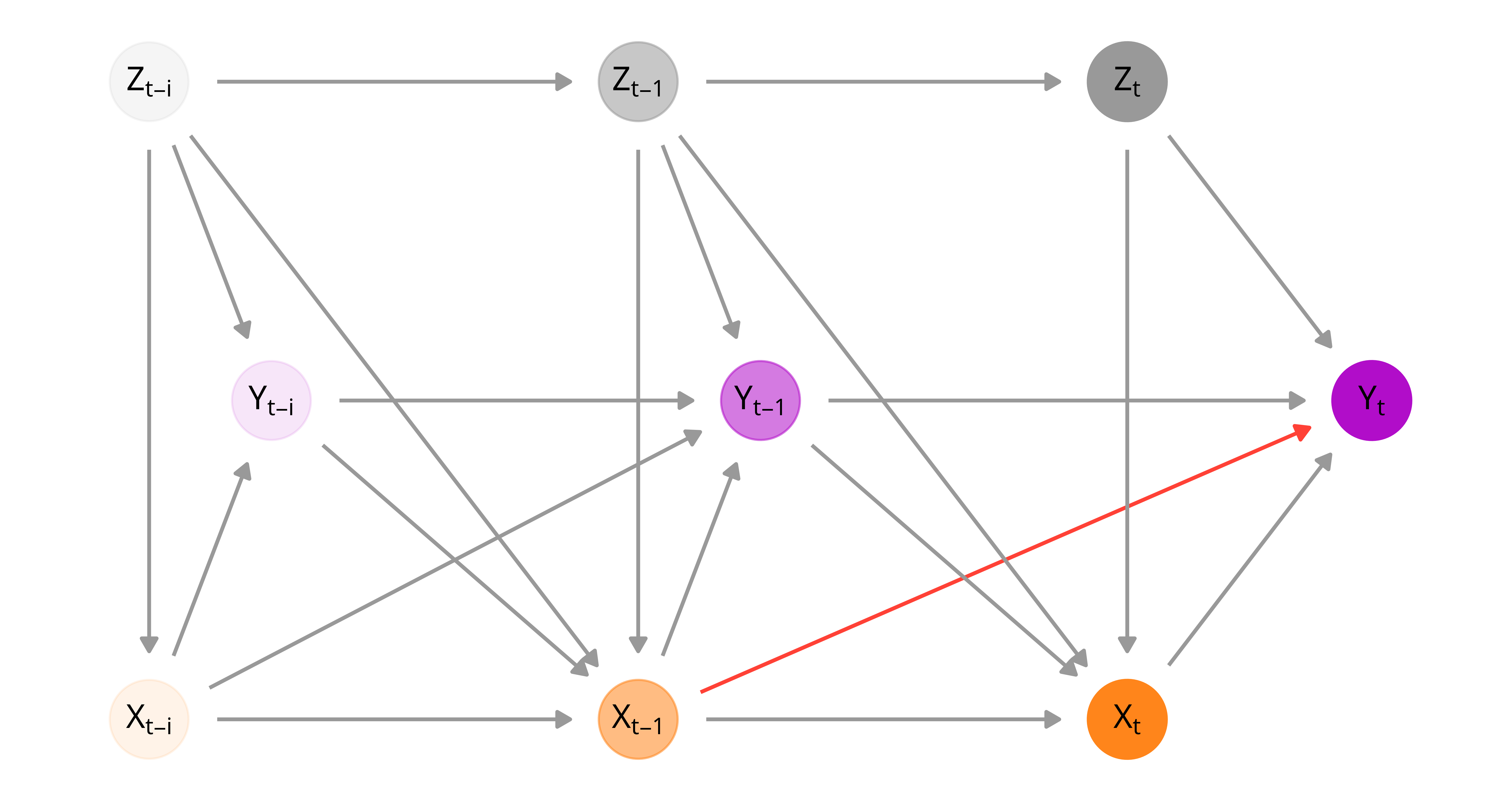
Doing this is tricky though. The relationship between a country’s history of civil society restrictions (\(X_{i, 1:t}\)) and the foreign aid it receives (\(Y_{it}\)) is confounded by time-varying confounders and previous levels of foreign aid, many of which are post-treatment covariates that cannot be directly adjusted for. The treatment model accounts for a bunch of confounders across three broader categories: (1) human rights and politics (like corruption, level of democracy, etc.), (2) economics and development (like trade, mortality, etc.), and (3) unexpected shocks (like natural disasters). This is based on the following DAG:
In order to calculate the total effect of restrictions in time \(t-1\) on foreign aid in time \(t\), we need to adjust for post-treatment confounders \(Z_t\). However, adjusting for post-treatment covariates is bad (Montgomery, Nyhan, and Torres 2018). Moreover, we believe that overall treatment history matters. More rapid changes in the civil society regulatory environment, or more severely restricted countries in general, should have a more sizable impact on donor country aid allocation decisions. Fortunately marginal structural models, first developed in epidemiology and biostatistics, allow us to account for both dynamic confounding and treatment history.
But before building any MSMs, we need to define our exact causal estimand. We follow the recommendation of Lundberg, Johnson, and Stewart (2021) and do this in three steps:
- Choose a theoretical estimand (\(\tau\)) and connect it to a general theory. It needs to describe a hypothetical intervention, a unit-specific quantity (like \(Y_i\) for a realized outcome or \(Y_i(1) - Y_i(0)\) for a potential outcome), and a target population (like \({\textstyle \frac{1}{n}}\ {\textstyle \sum_{i=1}^n}\))
- Choose an empirical estimand (\(\theta\)) that is linked to the theoretical estimand based on a set of identification assumptions from a DAG
- Choose an estimation strategy to learn the empirical estimand from the data. This is \(\hat{\theta}\).
Quick background reference: Potential outcomes, \(\operatorname{do}(\cdot)\), and causal effects
Before getting into the different estimands, here’s some quick translation between definitions of causal effects in the worlds of potential outcomes and DAGs. We can think of theoretical and empirical estimands in do-calculus terms like this:
A theoretical estimand often has \(\operatorname{do}(\cdot)\) operator in it (but not always). It represents data that isn’t observable, since with non-experimental data you cannot intervene directly to see \(E[Y \mid \operatorname{do}(X)]\) and you’re instead stuck with \(E[Y \mid X]\).
There are many situations where a theoretical estimand doesn’t have a \(\operatorname{do}(\cdot)\).1 For instance, if you’re interested in a population parameter and only have access to a sample, the theoretical estimand is the mean in the full population, while the empirical estimand is the sample mean. Missing data also does not involve \(\operatorname{do}(\cdot)\)—you might be interested in a parameter in the full population but only have the recorded non-missing observed data. In causal inference, though, where we’re interested in interventions and effects, theoretical estimands will have a \(\operatorname{do}(\cdot)\).
An empirical estimand uses the rules of do-calculus (backdoor adjustment, frontdoor adjustment, etc.) to create a do-free expression for observed data. This is also known as identification. This expression will incorporate information about confounders based on relationships in the DAG.
In section 2.4 of Neal (2020) (p. 15), there’s a flowchart of estimands that looks a lot like the estimand framework in Lundberg, Johnson, and Stewart (2021), just with different names:
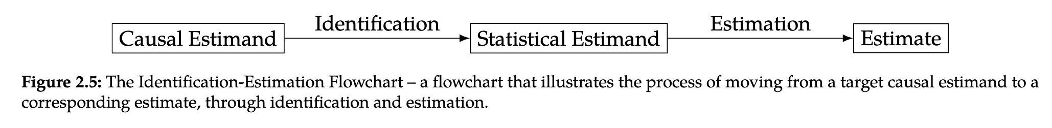
According to footnote 14 in that chapter, the causal estimand (which seems to map to the theoretical estimand) contains \(\operatorname{do}(\cdot)\), while the statistical estimand (which seems to map to the empirical estimand) does not. Based on this, we can translate do-calculus-style equations into potential outcomes-style equations like these general forms for binary and continuous average causal effects:
General forms for theoretical estimands
Binary treatments:
\[ \begin{aligned} & \textbf{ACEs in the potential outcomes world:} \\ \tau\ =&\ {\textstyle \frac{1}{n} \sum_{i=1}^n} Y_i (1) - Y_i (0) \\ & \\ & \text{or alternatively with } \textbf{E} \\ \tau\ =&\ \textbf{E} [Y_i (1) - Y_i (0)] \\ & \text{or}\\ =&\ \textbf{E} [Y_i^1 - Y_i^0] \\ & \\ & \textbf{ACEs in Pearl world:} \\ \tau(X)\ =&\ \textbf{E}[Y_i \mid \operatorname{do}(X = 1) - Y_i \mid \operatorname{do}(X = 0)] \\ & \text{or} \\ =&\ \textbf{E}[Y_i^{\operatorname{do}(x = 1)} - Y_i^{\operatorname{do}(x = 0)}] \\ & \\ & \text{or more simply} \\ =&\ \textbf{E} [Y_i \mid \operatorname{do}(X)] \\ \end{aligned} \]
Continuous treatments:
\[ \begin{aligned} & \textbf{ACEs in the potential outcomes world:} \\ \tau\ =&\ \textbf{E} [Y_i (t^\star) - Y_i (t)] \\ & \\ & \textbf{ACEs in Pearl world:} \\ \tau(t) =&\ \textbf{E}[Y_i \mid \operatorname{do}(t^\star) - Y_i \mid \operatorname{do}(t)] \\ & \text{where } t, t^\star \in \mathcal{T} \text{ and } \mathcal{T} = [\min(t), \max(t)] \\ & \\ & \text{or as an average dose response function:} \\ =&\ E[Y_i(t)] \end{aligned} \]
(Note, Pearl also uses an explicit \(\operatorname{do}(x + 1)\) for the counterfactual on p. 2 here (Pearl 2019) rather than a more arbitrary \(\operatorname{do}(x^\star)\))
General forms for empirical estimands
Binary treatments:
\[ \begin{aligned} & \textbf{Potential outcomes world:} \\ \theta\ =&\ \frac{1}{n_{X = 1}} \sum_{i \in \mathcal{S}_{X = 1}} Y_i - \frac{1}{n_{X = 0}} \sum_{i \in \mathcal{S}_{X = 0}} Y_i \\ & \\ & \text{or alternatively with } \textbf{E} \\ =&\ \textbf{E}[Y_i \mid X = 1)] - \textbf{E}[Y_i \mid X = 0] \\ & \\ & \textbf{Pearl world:} \\ \theta(X)\ =&\ \textbf{E}[Y_i \mid \operatorname{do}(X = 1)] - \textbf{E}[Y_i \mid \operatorname{do}(X = 0)] \rightarrow \\ & \\ & \text{assuming there are backdoor confounders } Z_i \text{ to remove } \operatorname{do}(X) \\ =&\ \sum_Z P(Y_i \mid X_i = 1, Z_i)\ P(Z_i) - \sum_Z P(Y_i \mid X_i = 0, Z_i)\ P(Z_i) \end{aligned} \]
Continuous treatments:
\[ \begin{aligned} & \textbf{Potential outcomes world:} \\ \theta\ =& \textbf{E} [Y_i (t^\star)] - \textbf{E}[Y_i (t)] \\ & \\ & \textbf{Pearl world:} \\ \theta(t) =& \textbf{E}[Y_i \mid \operatorname{do}(t^\star)] - \textbf{E}[Y_i \mid \operatorname{do}(t)] \\ \text{or just}\ & \textbf{E}[Y_i \mid \operatorname{do}(t)] \rightarrow \\ & \\ & \text{assuming there are backdoor confounders } Z_i \text{ to remove } \operatorname{do}(t) \\ \theta(t)\ =& \sum_Z P(Y_i \mid t, Z_i)\ P(Z_i) \\ & \\ & \text{where } t, t^\star \in \mathcal{T} \text{ and } \mathcal{T} = [\min(t), \max(t)] \end{aligned} \]
General forms for estimation strategy
There aren’t really any general forms for this. You figure out \(\hat{\theta}\) however is best. Regression, difference in means, inverse probability weighting, whatever.
1. Set the target: The theoretical estimand (\(\tau\))
First we have to define a theoretical estimand, which requires a substantive argument connected to theory. In this project, we care about the average difference in the potential outcome of foreign aid each aid-eligible country \(i\) would receive if that country increased its legal restrictions on NGOs in the previous year versus if it did not increase legal restrictions. We’re interested in the effect of an increase in the number of laws in the preceding year, along with the total cumulative number of laws (or the treatment history), for some number of periods \(T\). Equation 1 shows this theoretical estimand:
\[ \tau = \underbrace{{\textstyle \frac{1}{n}}\ {\textstyle \sum_{i=1}^n}}_{\substack{\text{mean over} \\ \text{all countries} \\ \text{eligible for aid}}} \bigg[ \underbrace{Y_{it} (x^\prime_{i, t-1:T})}_{\substack{\text{potential foreign aid} \\ \text{with alternative} \\ \text{NGO legal history}}} - \underbrace{Y_{it} (x_{i, t-1:T})}_{\substack{\text{potential foreign aid} \\ \text{with actual} \\ \text{NGO legal history}}} \bigg] \tag{1}\]
Or, following Pearl (2019), a do-based version of the same thing:
\[ \begin{aligned} \tau =& \underbrace{\textbf{E}}_{\substack{\text{Expectation} \\ \text{for all countries} \\ \text{eligible for aid}}} \bigg[ \underbrace{Y_{it} \mid \operatorname{do} (x^\prime_{i, t-1:T})}_{\substack{\text{Causal effect} \\ \text{with alternative} \\ \text{NGO legal history}}} - \underbrace{Y_{it} \mid \operatorname{do} (x_{i, t-1:T})}_{\substack{\text{Causal effect of} \\ \text{actual NGO legal} \\ \text{history on foreign aid}}} \bigg] \end{aligned} \tag{2}\]
We thus have these key definitions for our theoretical estimand:
- Target population of units (\(i\)): All countries eligible to receive foreign aid
- Unit-specific quantity: Difference between foreign aid that country \(i\) would receive if it passed an anti-NGO law vs. if it didn’t
Because it is not possible to observe both potential outcomes for each country, the theoretical estimand \(\tau\) is unmeasurable. But that’s fine! Theoretical estimands don’t need to be measurable. That’s what the empirical estimand is for.
2. Empirical estimand: Link to observables (\(\theta\))
Next, we move from the theoretical estimand to an empirical estimand, which requires conceptual assumptions based on the DAG. Our empirical estimand is the difference in average observed outcomes across countries in time \(t\) as the observed count of NGO laws changes in time \(t-1\) and modifies the overall treatment history, all conditional on confounders \(Z\)
\[ \theta =\ \underbrace{\textbf{E}_Z}_{\substack{\text{Expectation} \\ \text{conditional} \\ \text{on observed} \\ \text{confounders }Z}} \bigg[ \underbrace{\textbf{E}[Y_{it} \mid X_{i,t-1:T} = X_{i,t-1:T} + 1, Z]}_{\substack{\text{Observed mean aid given} \\ \text{total NGO laws in } t-1 \\ {\textbf{plus one hypothetical extra law}}}} - \underbrace{\textbf{E}[Y_{it} \mid X_{i, t-1:T, Z}]}_{\substack{\text{Observed mean aid given} \\ \text{total NGO laws in } t-1}} \bigg] \tag{3}\]
3. Learn from the data (\(\hat{\theta}\))
We find \(\hat{\theta}\) by defining an estimation strategy and providing statistical evidence. We estimate \(\hat{\theta}\) using a marginal structural model (MSM) and inverse probability of treatment weights (IPTW). There’s a whole literature in epidemiology and biostats about how these work and how they provide unbiased estimates of causal parameters through g-estimation. In summary (see equation 32 in Blackwell and Glynn (2018)), using stabilized inverse probability weights based on confounders \(Z\) in a MSM makes it so that the expectation of \(Y_{it}\) conditional on \(X_{i, t-1}\) converges to the true empirical estimand:
\[ \hat{\theta} =\ \underbrace{\textbf{E}_\text{SW}[Y_{it} \mid X_{i, t-1} = x_{t-1}]}_{\substack{\text{observed average aid} \\ \text{given reweighted treatment}}} \xrightarrow{p} \underbrace{\textbf{E}[Y_{it} (x_{t-1})]}_{\substack{\text{this is kinda} \\ \text{like } \tau \text{ or } \theta?}} \tag{4}\]
The biostats g-estimation way of writing this MSM looks like this:
\[ \begin{aligned} \hat{\theta} &=\ \hat{g}(x_{t-1:T} + 1; \hat{\beta}) - \hat{g}(x_{t-1:T}; \hat{\beta}), \\ & \\ &\text{where} \\ & \\ \hat{\beta} &=\ (\hat{\beta_0} + \hat{\beta_1} x_{i, t-1}) \times \text{IPTW}_{i, t-1:T}, \\ & \\ &\text{which simplifies to} \\ & \\ \hat{\theta} &=\ \underbrace{\hat{\beta_1}}_{\substack{\text{average} \\ \text{causal} \\ \text{effect}}} \end{aligned} \tag{5}\]
We can thus obtain an unbiased estimate of the causal parameter \(\beta_1\) of the MSM by giving each country a country- and time-specific weight, based on the confounders.
All estimands
Thus, here’s our Lundberg, Johnson, and Stewart (2021) process:
Theoretical, unobservable estimand (\(\tau\)):
\[ \tau = \underbrace{{\textstyle \frac{1}{n}}\ {\textstyle \sum_{i=1}^n}}_{\substack{\text{Mean over} \\ \text{all countries} \\ \text{eligible for aid}}} \bigg[ \underbrace{Y_{it} (x^\prime_{i, t-1:T})}_{\substack{\text{Potential foreign aid} \\ \text{with alternative} \\ \text{NGO legal history}}} - \underbrace{Y_{it} (x_{i, t-1:T})}_{\substack{\text{Potential foreign aid} \\ \text{with actual} \\ \text{NGO legal history}}} \bigg] \tag{6}\]
\[ \begin{aligned} \tau =& \underbrace{\textbf{E}}_{\substack{\text{Expectation} \\ \text{for all countries} \\ \text{eligible for aid}}} \bigg[ \underbrace{Y_{it} \mid \operatorname{do} (x^\prime_{i, t-1:T})}_{\substack{\text{Causal effect} \\ \text{with alternative} \\ \text{NGO legal history}}} - \underbrace{Y_{it} \mid \operatorname{do} (x_{i, t-1:T})}_{\substack{\text{Causal effect of} \\ \text{actual NGO legal} \\ \text{history on foreign aid}}} \bigg] \end{aligned} \tag{7}\]
Empirical estimand (\(\theta\)):
\[ \theta =\ \underbrace{\textbf{E}_Z}_{\substack{\text{Expectation} \\ \text{conditional} \\ \text{on observed} \\ \text{confounders }Z}} \bigg[ \underbrace{\textbf{E}[Y_{it} \mid X_{i,t-1:T} = X_{i,t-1:T} + 1, Z]}_{\substack{\text{Observed mean aid given} \\ \text{total NGO laws in } t-1 \\ {\textbf{plus one hypothetical extra law}}}} - \underbrace{\textbf{E}[Y_{it} \mid X_{i, t-1:T, Z}]}_{\substack{\text{Observed mean aid given} \\ \text{total NGO laws in } t-1}} \bigg] \tag{8}\]
Estimate of estimand (\(\hat{\theta}\)):
\[ \begin{aligned} \hat{\theta} &=\ \hat{g}(x_{t-1:T} + 1; \hat{\beta}) - \hat{g}(x_{t-1:T}; \hat{\beta}), \\ & \\ &\text{where} \\ & \\ \hat{\beta} &=\ (\hat{\beta_0} + \hat{\beta_1} x_{i, t-1}) \times \text{IPTW}_{i, t-1:T}, \\ & \\ &\text{which simplifies to} \\ & \\ \hat{\theta} &=\ \underbrace{\hat{\beta_1}}_{\substack{\text{average} \\ \text{causal} \\ \text{effect}}} \end{aligned} \tag{9}\]
References
Blackwell, Matthew, and Adam N. Glynn. 2018. “How to Make Causal Inferences with Time-Series Cross-Sectional Data Under Selection on Observables.” American Political Science Review 112 (4): 1067–82. https://doi.org/10.1017/s0003055418000357.
Kropko, Jonathan, and Robert Kubinec. 2020. “Interpretation and Identification of Within-Unit and Cross-Sectional Variation in Panel Data Models.” PLoS ONE 15 (4): 1–22. https://doi.org/10.1371/journal.pone.0231349.
Lundberg, Ian, Rebecca Johnson, and Brandon M. Stewart. 2021. “What Is Your Estimand? Defining the Target Quantity Connects Statistical Evidence to Theory.” American Sociological Review 86 (3): 532–65. https://doi.org/10.1177/00031224211004187.
Montgomery, Jacob M., Brendan Nyhan, and Michelle Torres. 2018. “How Conditioning on Posttreatment Variables Can Ruin Your Experiment and What to Do about It.” American Journal of Political Science 62 (3): 760–75. https://doi.org/10.1111/ajps.12357.
Muff, Stefanie, Leonhard Held, and Lukas F. Keller. 2016. “Marginal or Conditional Regression Models for Correlated Non-Normal Data?” Methods in Ecology and Evolution 7 (12): 1514–24. https://doi.org/10.1111/2041-210X.12623.
Neal, Brady. 2020. Introduction to Causal Inference from a Machine Learning Perspective. https://www.bradyneal.com/causal-inference-course.
Pearl, Judea. 2019. “On the Interpretation of Do(x).” Journal of Causal Inference 7 (1): 1–6. https://doi.org/10.1515/jci-2019-2002.
Footnotes
Thanks to Brandon Stewart and Ian Lundberg for clarifying this!↩︎