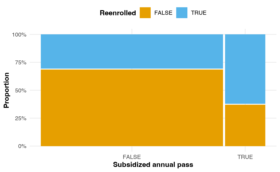
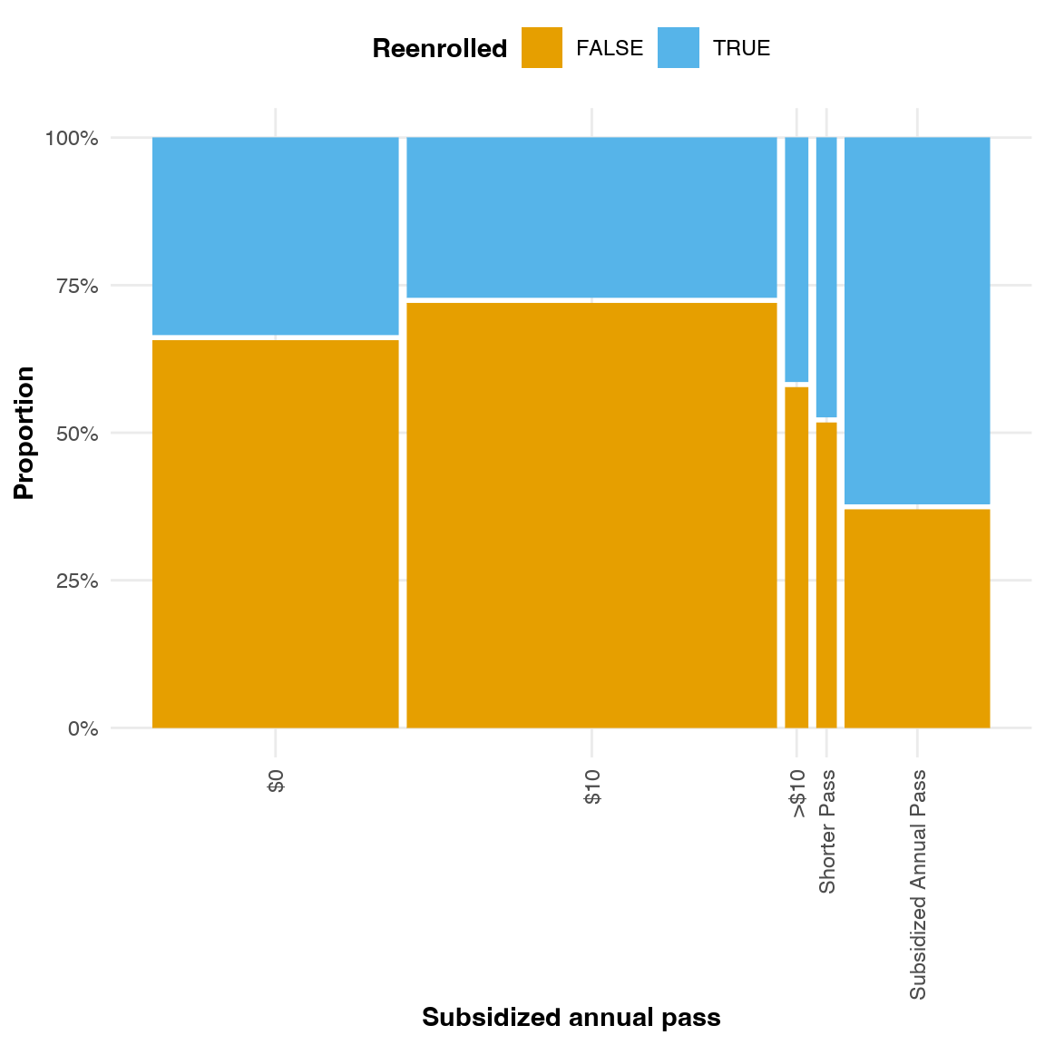
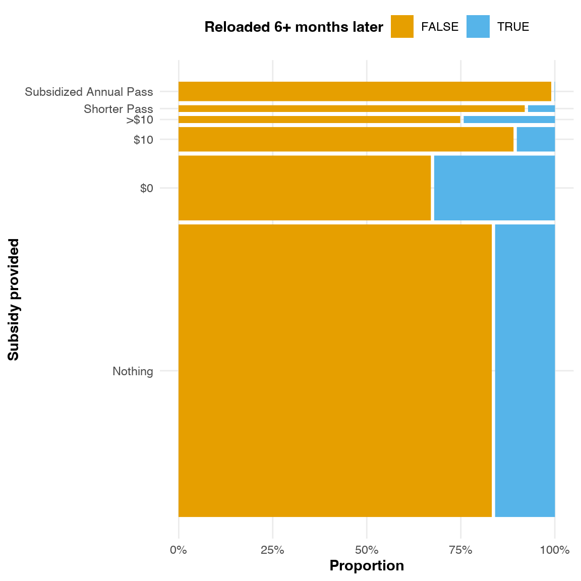
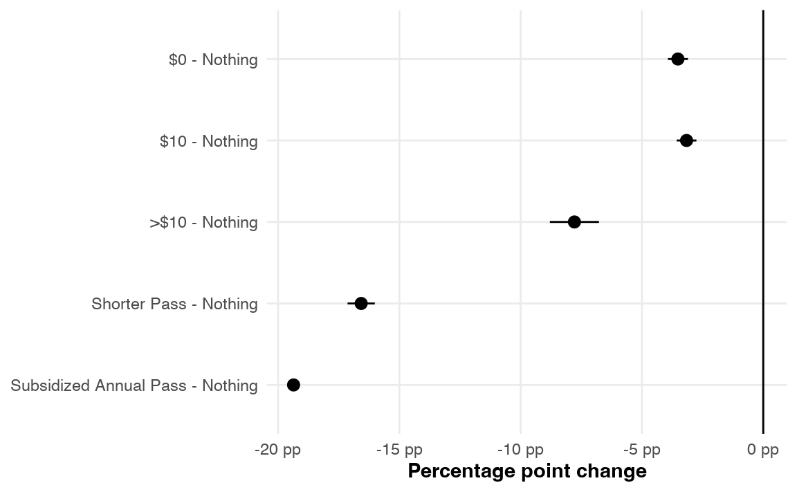
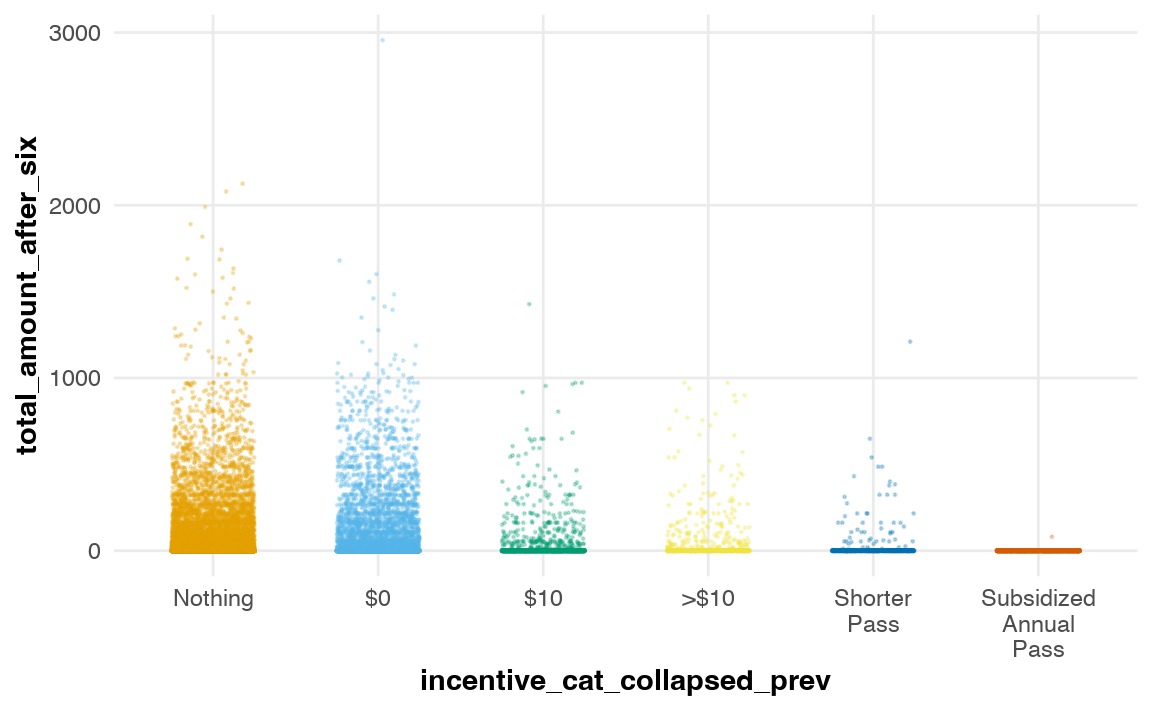
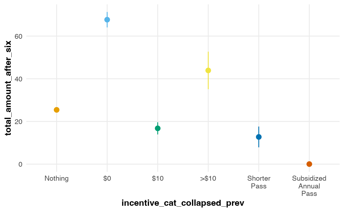
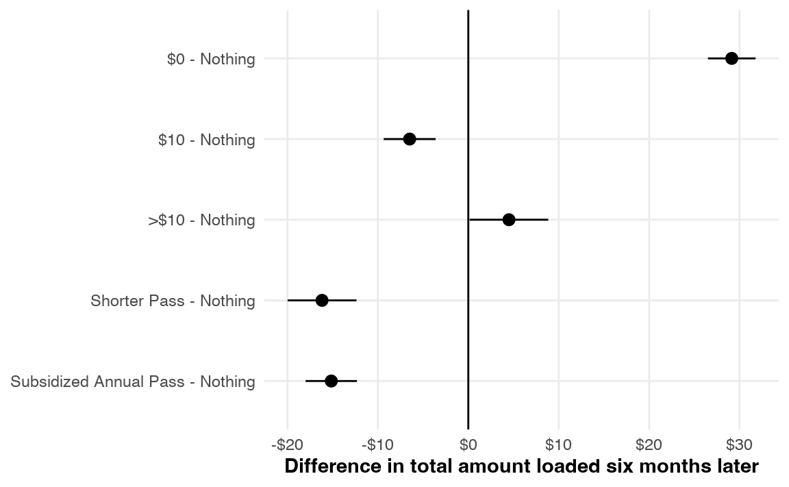
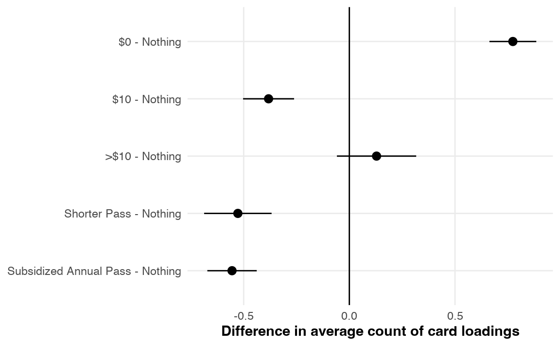
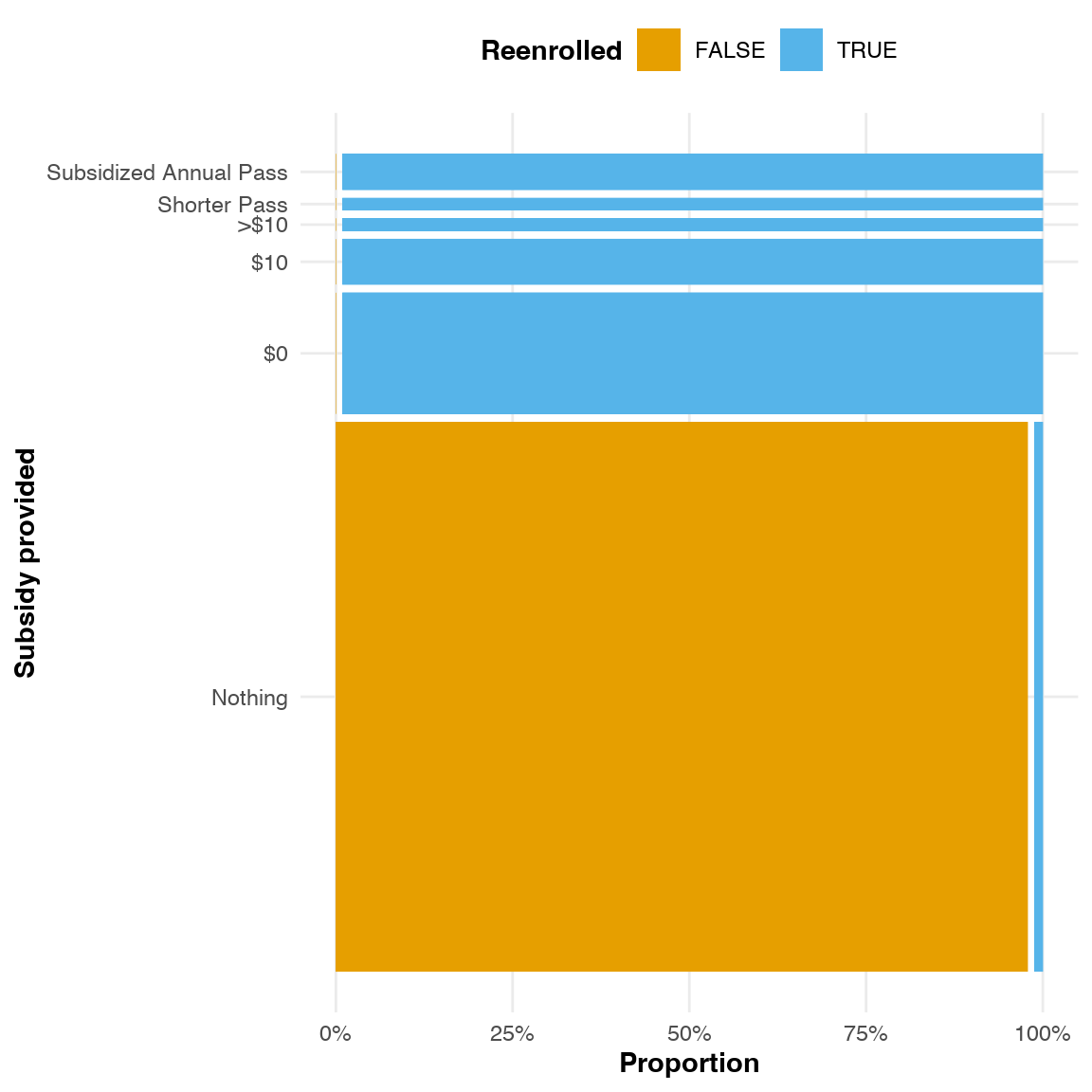
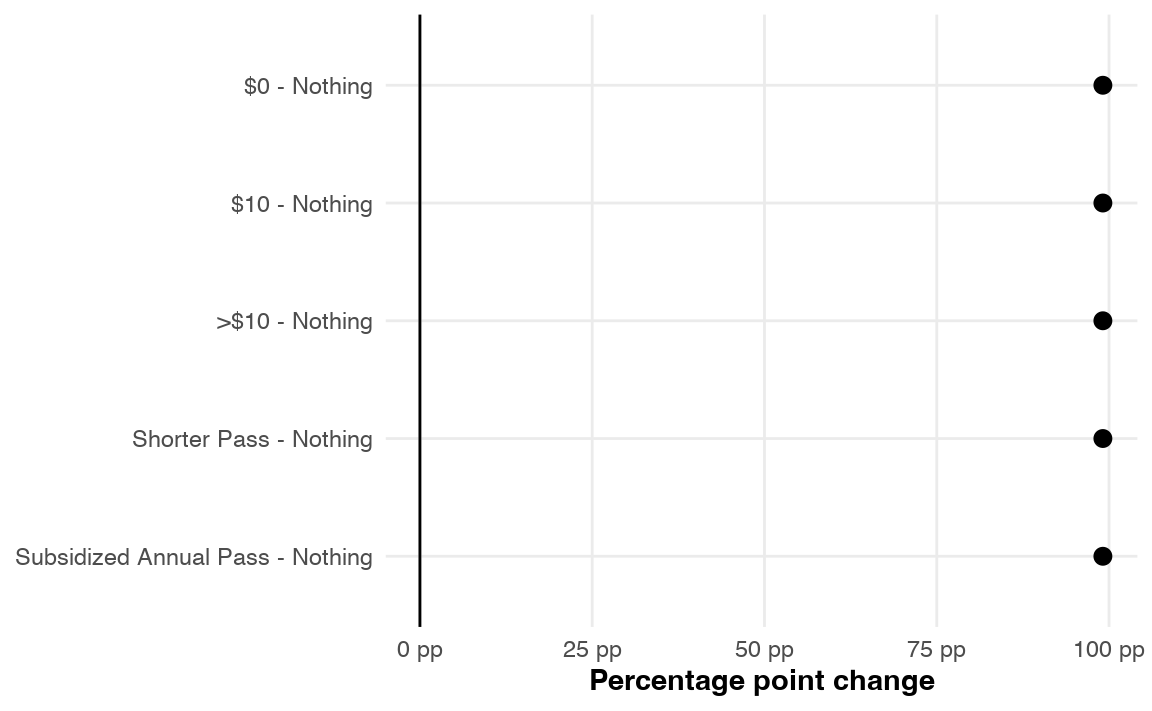
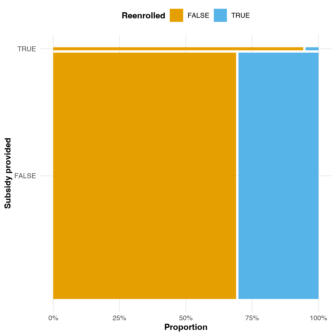
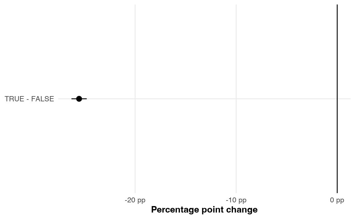
Q2: Effect of subsidies on enrollment

Code

library(tidyverse)
library(sf)
library(kableExtra)
library(ggmosaic)
library(gghalves)
library(ggokabeito)
library(scales)
library(lubridate)
library(here)
library(broom)
library(lme4)
library(broom.mixed)
library(WeightIt)
library(marginaleffects)
library(modelsummary)

riders_final <- readRDS(here("data", "derived_data", "riders_final.rds"))
riders_final_2019 <- readRDS(here("data", "derived_data", "riders_final_2019.rds"))
wa_bgs <- readRDS(here("data", "derived_data", "washington_block-groups.rds"))
acs_wa <- readRDS(here("data", "derived_data", "washington_acs.rds"))

# By default, R uses polynomial contrasts for ordered factors in linear models:
# > options("contrasts") 
# So we make ordered factors use treatment contrasts instead
options(contrasts = rep("contr.treatment", 2))

theme_kc <- function() {
  theme_minimal() +
    theme(panel.grid.minor = element_blank(),
          plot.background = element_rect(fill = "white", color = NA),
          plot.title = element_text(face = "bold"),
          axis.title = element_text(face = "bold"),
          strip.text = element_text(face = "bold"),
          strip.background = element_rect(fill = "grey80", color = NA),
          legend.title = element_text(face = "bold"))
}

riders_model <- riders_final_2019 %>% 
  select(load_after_six, total_amount_after_six, total_loadings_after_six, 
         reenrolled, treatment_passport_binary, treatment_passport_binary,
         incentive_cat_collapsed, incentive_cat_collapsed_prev, treatment_sap_binary,
         total_amount_before_six, total_loadings_before_six, enrolled_previously,
         boardings_king_county_before_six, boardings_sound_transit_before_six,
         Age, RaceDesc, LanguageSpoken, id, 
         bg_pct_white, bg_pct_male, bg_pct_hs, bg_pct_ba, 
         bg_internet, bg_travel_time_per_capita, bg_pub_trans_per_capita, 
         bg_income, bg_median_rent) %>% 
  na.omit()

Initial trends

Distribution of incentives

Code

incentives_2019 <- riders_final_2019 %>% 
  count(incentive_cat, name = "count_2019")

incentives_all <- riders_final %>% 
  count(incentive_cat, name = "count_all")

incentives_combined <- incentives_all %>% 
  left_join(incentives_2019, by = "incentive_cat")  %>%
  mutate(diff = count_all - count_2019)

incentives_combined %>% 
  kbl() %>% 
  kable_styling()

incentive_cat	count_all	count_2019	diff
$0	53524	18745	34779
$10	44263	28205	16058
$15	3849	596	3253
$20	645	451	194
$30	120	117	3
$50	422	415	7
$70	169	169	0
Misc. Pass	37	37	0
Monthly Pass	1888	668	1220
Passport	824	824	0
Subsidized Annual Pass	11050	11050	0

Only subsidized annual pass:

Code

ggplot(data = riders_final_2019) +
  geom_mosaic(aes(x = product(treatment_sap_binary), fill = ever_reenroll), alpha = 1) +
  scale_y_continuous(labels = scales::percent) +
  scale_fill_okabe_ito() +
  labs(x = "Subsidized annual pass", y = "Proportion", fill = "Reenrolled") +
  theme_kc() +
  theme(legend.position = "top")

All incentive categories:

Code

ggplot(data = riders_final_2019) +
  geom_mosaic(aes(x = product(incentive_cat_collapsed), fill = ever_reenroll), alpha = 1) +
  scale_y_continuous(labels = scales::percent) +
  scale_fill_okabe_ito() +
  labs(x = "Subsidized annual pass", y = "Proportion", fill = "Reenrolled") +
  theme_kc() +
  theme(axis.text.x = element_text(angle = 90, hjust = 1, vjust = 0.5),
        legend.position = "top")

Q2_A: Effect of different levels of incentives on longer-term loading of value and passes

Outcomes representing long term loading:

• load_after_six: Binary indicator for whether they reloaded the card 6+ months after card is issued
• total_amount_after_six: Amount of money refilled 6+ months after card is issued
• total_loadings_after_six: Count of refills 6+ months after card is issued

Treatment:

• incentive_cat_collapsed: Categorical variable showing the kind of incentive each person was given with the card, if any. Possible values are 0, 10, 10+ (15, 20, 30, 50, 70), Shorter Pass (Misc. Pass, Monthly Pass, Passport), and Subsidized Annual Pass; the values are ordered based on their intensity

IPW

Code

incentive_weights <- weightit(
  incentive_cat_collapsed_prev ~ Age + RaceDesc + LanguageSpoken + 
    total_amount_before_six + total_loadings_before_six + enrolled_previously +
    boardings_king_county_before_six + boardings_sound_transit_before_six +
    bg_pct_white + bg_pct_male + bg_pct_hs + bg_pct_ba + bg_internet + 
    bg_travel_time_per_capita + bg_pub_trans_per_capita + bg_income + bg_median_rent,
  data = riders_model, estimand = "ATE", method = "ps")
## Warning: glm.fit: fitted probabilities numerically 0 or 1 occurred

riders_model_with_weights <- riders_model %>% 
  mutate(ipw = incentive_weights$weights) %>% 
  mutate(ipw = ifelse(ipw >= 30, 30, ipw))

Code

passport_weights <- weightit(
  treatment_passport_binary ~ Age + RaceDesc + LanguageSpoken + 
    total_amount_before_six + total_loadings_before_six + enrolled_previously +
    boardings_king_county_before_six + boardings_sound_transit_before_six +
    bg_pct_white + bg_pct_male + bg_pct_hs + bg_pct_ba + bg_internet + 
    bg_travel_time_per_capita + bg_pub_trans_per_capita + bg_income + bg_median_rent,
  data = riders_model, estimand = "ATE", method = "ps")
## Warning: glm.fit: fitted probabilities numerically 0 or 1 occurred
## Warning: Some extreme weights were generated. Examine them with summary() and maybe trim
## them with trim().

passport_model_with_weights <- riders_model %>% 
  mutate(ipw = passport_weights$weights) %>% 
  mutate(ipw = ifelse(ipw >= 30, 30, ipw))

Reloading after 6 months

Code

ggplot(riders_model) +
  geom_mosaic(aes(x = product(incentive_cat_collapsed_prev), fill = load_after_six), alpha = 1) +
  scale_y_continuous(labels = scales::percent) +
  scale_fill_okabe_ito() +
  labs(x = "Subsidy provided", y = "Proportion", fill = "Reloaded 6+ months later") +
  theme_kc() +
  theme(legend.position = "top") +
  coord_flip()

Code

model_q2a_1 <- glmer(load_after_six ~ incentive_cat_collapsed_prev + (1 | id),
                     family = binomial(link = "logit"),
                     data = riders_model_with_weights, weights = ipw)
## Warning in eval(family$initialize, rho): non-integer #successes in a binomial glm!

Code

tidy(model_q2a_1) %>% 
  kbl() %>% 
  kable_styling()

effect	group	term	estimate	std.error	statistic	p.value
fixed	NA	(Intercept)	-10.63	0.063	-169.8	0
fixed	NA	incentive_cat_collapsed_prev$0	-2.08	0.080	-25.9	0
fixed	NA	incentive_cat_collapsed_prev$10	-1.93	0.086	-22.5	0
fixed	NA	incentive_cat_collapsed_prev>$10	-3.56	0.153	-23.3	0
fixed	NA	incentive_cat_collapsed_prevShorter Pass	-7.08	0.186	-38.1	0
fixed	NA	incentive_cat_collapsed_prevSubsidized Annual Pass	-13.43	0.521	-25.8	0
ran_pars	id	sd__(Intercept)	27.12	NA	NA	NA

Code

model_q2a_1_cmp <- comparisons(model_q2a_1, 
                                variables = "incentive_cat_collapsed_prev", 
                                contrast_factor = "reference")
model_q2a_1_cmp %>% 
  tidy() %>% 
  mutate(contrast = fct_rev(fct_inorder(contrast))) %>% 
  ggplot(aes(x = estimate * 100, y = contrast)) +
  geom_vline(xintercept = 0) +
  geom_pointrange(aes(xmin = conf.low * 100, xmax = conf.high * 100)) +
  scale_x_continuous(labels = ~paste0(.x, " pp")) +
  labs(x = "Percentage point change", y = NULL) +
  theme_kc()

Total amount refilled after 6 months

Code

avg_after_6 <- riders_model %>% 
  group_by(incentive_cat_collapsed_prev) %>% 
  summarize(avg_amount = mean(total_amount_after_six),
            se_amount = sd(total_amount_after_six) / sqrt(n()),
            hi_lo_amount = map2(avg_amount, se_amount, 
                                ~.x + (.y * qnorm(c(0.025, 0.975)))),
            avg_loadings = mean(total_loadings_after_six),
            se_loadings = sd(total_loadings_after_six) / sqrt(n()),
            hi_lo_loadings = map2(avg_loadings, se_loadings, 
                                  ~.x + (.y * qnorm(c(0.025, 0.975)))),)
avg_after_6 %>% 
  kbl() %>% 
  kable_styling()

incentive_cat_collapsed_prev	avg_amount	se_amount	hi_lo_amount	avg_loadings	se_loadings	hi_lo_loadings
Nothing	25.433	0.536	24.4, 26.5	1.069	0.025	1.02, 1.12
$0	67.683	1.846	64.1, 71.3	2.395	0.068	2.26, 2.53
$10	16.775	1.452	13.9, 19.6	0.679	0.071	0.540, 0.818
>$10	43.910	4.486	35.1, 52.7	1.795	0.244	1.32, 2.27
Shorter Pass	12.748	2.483	7.88, 17.61	0.384	0.080	0.228, 0.541
Subsidized Annual Pass	0.032	0.032	-0.0311, 0.0959	0.001	0.001	-0.000778, 0.002399

Code

ggplot(riders_model, aes(x = incentive_cat_collapsed_prev, 
                         y = total_amount_after_six, 
                         color = incentive_cat_collapsed_prev)) +
  geom_point(size = 0.2, alpha = 0.25, 
             position = position_jitter(width = 0.25, seed = 1234)) +
  scale_color_okabe_ito(guide = "none") +
  scale_x_discrete(labels = label_wrap(10)) +
  theme_kc()

Code

ggplot(riders_model, aes(x = incentive_cat_collapsed_prev, 
                         y = total_amount_after_six, 
                         color = incentive_cat_collapsed_prev)) +
  stat_summary(geom = "pointrange", fun.data = "mean_se", fun.args = list(mult = 1.96)) +
  scale_color_okabe_ito(guide = "none") +
  scale_x_discrete(labels = label_wrap(10)) +
  theme_kc()

Code

model_q2a_2 <- lmer(total_amount_after_six ~ incentive_cat_collapsed_prev + (1 | id),
                    data = riders_model_with_weights, weights = ipw)

Code

tidy(model_q2a_2) %>% 
  kbl() %>% 
  kable_styling()

effect	group	term	estimate	std.error	statistic
fixed	NA	(Intercept)	28.77	0.686	41.97
fixed	NA	incentive_cat_collapsed_prev$0	29.14	1.344	21.67
fixed	NA	incentive_cat_collapsed_prev$10	-6.49	1.466	-4.42
fixed	NA	incentive_cat_collapsed_prev>$10	4.50	2.217	2.03
fixed	NA	incentive_cat_collapsed_prevShorter Pass	-16.18	1.942	-8.33
fixed	NA	incentive_cat_collapsed_prevSubsidized Annual Pass	-15.15	1.449	-10.46
ran_pars	id	sd__(Intercept)	69.56	NA	NA
ran_pars	Residual	sd__Observation	132.56	NA	NA

Code

model_q2a_2_cmp <- comparisons(model_q2a_2, 
                               variables = "incentive_cat_collapsed_prev", 
                               contrast_factor = "reference")
model_q2a_2_cmp %>% 
  tidy() %>% 
  mutate(contrast = fct_rev(fct_inorder(contrast))) %>% 
  ggplot(aes(x = estimate, y = contrast)) +
  geom_vline(xintercept = 0) +
  geom_pointrange(aes(xmin = conf.low, xmax = conf.high)) +
  scale_x_continuous(labels = label_dollar()) +
  labs(x = "Difference in total amount loaded six months later", y = NULL) +
  theme_kc()

Total loadings after 6 months

Code

model_q2a_3 <- lmer(total_loadings_after_six ~ incentive_cat_collapsed_prev + (1 | id),
                    data = riders_model_with_weights, weights = ipw)

Code

tidy(model_q2a_3) %>% 
  kbl() %>% 
  kable_styling()

effect	group	term	estimate	std.error	statistic
fixed	NA	(Intercept)	1.206	0.029	41.71
fixed	NA	incentive_cat_collapsed_prev$0	0.774	0.057	13.68
fixed	NA	incentive_cat_collapsed_prev$10	-0.382	0.062	-6.21
fixed	NA	incentive_cat_collapsed_prev>$10	0.129	0.096	1.34
fixed	NA	incentive_cat_collapsed_prevShorter Pass	-0.528	0.081	-6.48
fixed	NA	incentive_cat_collapsed_prevSubsidized Annual Pass	-0.555	0.060	-9.31
ran_pars	id	sd__(Intercept)	3.244	NA	NA
ran_pars	Residual	sd__Observation	5.360	NA	NA

Code

model_q2a_3_cmp <- comparisons(model_q2a_3, 
                               variables = "incentive_cat_collapsed_prev", 
                               contrast_factor = "reference")
model_q2a_3_cmp %>% 
  tidy() %>% 
  mutate(contrast = fct_rev(fct_inorder(contrast))) %>% 
  ggplot(aes(x = estimate, y = contrast)) +
  geom_vline(xintercept = 0) +
  geom_pointrange(aes(xmin = conf.low, xmax = conf.high)) +
  labs(x = "Difference in average count of card loadings", y = NULL) +
  theme_kc()

All models

Code

modelsummary(list("Reload (binary)" = model_q2a_1,
                  "Amount refilled" = model_q2a_2,
                  "Loadings" = model_q2a_3))

	Reload (binary)	Amount refilled	Loadings
(Intercept)	−10.635	28.774	1.206
	(0.063)	(0.686)	(0.029)
incentive_cat_collapsed_prev$0	−2.084	29.135	0.774
	(0.080)	(1.344)	(0.057)
incentive_cat_collapsed_prev$10	−1.932	−6.485	−0.382
	(0.086)	(1.466)	(0.062)
incentive_cat_collapsed_prev>$10	−3.559	4.498	0.129
	(0.153)	(2.217)	(0.096)
incentive_cat_collapsed_prevShorter Pass	−7.080	−16.177	−0.528
	(0.186)	(1.942)	(0.081)
incentive_cat_collapsed_prevSubsidized Annual Pass	−13.426	−15.153	−0.555
	(0.521)	(1.449)	(0.060)
sd__(Intercept)	27.121	69.563	3.244
sd__Observation		132.555	5.360
Num.Obs.	53152	53152	53152
AIC	50145.9	662962.3	326576.5
BIC	50208.1	663033.3	326647.5
Log.Lik.	−25065.964	−331473.136	−163280.234
REMLcrit		662946.273	326560.467

Q2_B: Effect of different levels of incentives on longer-term loading of value and passes

Outcome:

• reenrolled: Binary indicator for whether current card issuing is a reenrollment (TRUE when the suffix for the card ID is greater than 1)

Code

ggplot(riders_model) +
  geom_mosaic(aes(x = product(incentive_cat_collapsed_prev), fill = reenrolled), alpha = 1) +
  scale_y_continuous(labels = scales::percent) +
  scale_fill_okabe_ito() +
  labs(x = "Subsidy provided", y = "Proportion", fill = "Reenrolled") +
  theme_kc() +
  theme(legend.position = "top") +
  coord_flip()

Code

riders_model %>% 
  group_by(incentive_cat_collapsed_prev) %>% 
  summarize(prop = mean(reenrolled)) %>% 
  kbl() %>% 
  kable_styling()

?(caption)

incentive_cat_collapsed_prev	prop
Nothing	0.012
$0	1.000
$10	1.000
>$10	1.000
Shorter Pass	1.000
Subsidized Annual Pass	1.000

Code

model_q2b <- glmer(reenrolled ~ incentive_cat_collapsed_prev + (1 | id),
                   family = binomial(link = "logit"),
                   data = riders_model_with_weights, weights = ipw)
## Warning in eval(family$initialize, rho): non-integer #successes in a binomial glm!
## Warning in checkConv(attr(opt, "derivs"), opt$par, ctrl = control$checkConv, : Model
## failed to converge with max|grad| = 18.305 (tol = 0.002, component 1)

Code

tidy(model_q2b) %>% 
  kbl() %>% 
  kable_styling()

effect	group	term	estimate	std.error	statistic	p.value
fixed	NA	(Intercept)	-11.52	0.247	-46.70	0
fixed	NA	incentive_cat_collapsed_prev$0	26.33	1.782	14.78	0
fixed	NA	incentive_cat_collapsed_prev$10	28.32	4.843	5.85	0
fixed	NA	incentive_cat_collapsed_prev>$10	25.37	1.136	22.33	0
fixed	NA	incentive_cat_collapsed_prevShorter Pass	25.96	1.565	16.59	0
fixed	NA	incentive_cat_collapsed_prevSubsidized Annual Pass	25.09	1.107	22.67	0
ran_pars	id	sd__(Intercept)	9.41	NA	NA	NA

Code

model_q2b_cmp <- comparisons(model_q2b, 
                             variables = "incentive_cat_collapsed_prev", 
                             contrast_factor = "reference")
model_q2b_cmp %>% 
  tidy() %>% 
  mutate(contrast = fct_rev(fct_inorder(contrast))) %>% 
  ggplot(aes(x = estimate * 100, y = contrast)) +
  geom_vline(xintercept = 0) +
  geom_pointrange(aes(xmin = conf.low * 100, xmax = conf.high * 100)) +
  scale_x_continuous(labels = ~paste0(.x, " pp")) +
  labs(x = "Percentage point change", y = NULL) +
  theme_kc()

lol i have no idea what’s happening here

Q2_C: Effect of different levels of incentives on longer-term loading of value and passes

Outcome:

• reenrolled: Binary indicator for whether current card issuing is a reenrollment (TRUE when the suffix for the card ID is greater than 1)

Code

ggplot(passport_model_with_weights) +
  geom_mosaic(aes(x = product(treatment_passport_binary), fill = reenrolled), alpha = 1) +
  scale_y_continuous(labels = scales::percent) +
  scale_fill_okabe_ito() +
  labs(x = "Subsidy provided", y = "Proportion", fill = "Reenrolled") +
  theme_kc() +
  theme(legend.position = "top") +
  coord_flip()

Code

model_q2c_4 <- glmer(reenrolled ~ treatment_passport_binary + (1 | id),
                     family = binomial(link = "logit"),
                     data = passport_model_with_weights, weights = ipw)
## Warning in eval(family$initialize, rho): non-integer #successes in a binomial glm!

Code

tidy(model_q2c_4) %>% 
  kbl() %>% 
  kable_styling()

effect	group	term	estimate	std.error	statistic	p.value
fixed	NA	(Intercept)	-1.38	0.025	-56.2	0
fixed	NA	treatment_passport_binaryTRUE	-4.02	0.115	-35.0	0
ran_pars	id	sd__(Intercept)	1.43	NA	NA	NA

Code

model_q2c_4_cmp <- comparisons(model_q2c_4, 
                               variables = "treatment_passport_binary", 
                               contrast_factor = "reference")
model_q2c_4_cmp %>% 
  tidy() %>% 
  mutate(contrast = fct_rev(fct_inorder(contrast))) %>% 
  ggplot(aes(x = estimate * 100, y = contrast)) +
  geom_vline(xintercept = 0) +
  geom_pointrange(aes(xmin = conf.low * 100, xmax = conf.high * 100)) +
  scale_x_continuous(labels = ~paste0(.x, " pp")) +
  labs(x = "Percentage point change", y = NULL) +
  theme_kc()