Exploratory data analysis

Code
library(tidyverse)
library(tigris)
library(sf)
library(lubridate)
library(here)

riders_final <- readRDS(here("data", "derived_data", "riders_final.rds"))
riders_final_2019 <- readRDS(here("data", "derived_data", "riders_final_2019.rds"))
wa_bgs <- readRDS(here("data", "derived_data", "washington_block-groups.rds"))
acs_wa <- readRDS(here("data", "derived_data", "washington_acs.rds"))
Code
# Seattle-area counties
seattle_counties <- c("King", "Snohomish", "Pierce", "Kitsap", "Chelan", "Kittitas")

wa_counties <- counties(state = 53, year = 2019)

seattle_water <- tibble(county = seattle_counties) %>% 
  # Get each county individually
  mutate(water = map(county, ~area_water("WA", .x, year = 2019))) %>% 
  unnest(water) %>% 
  st_sf()  # Make the geometry column magical again

Number of people who reenrolled:

Code
riders_final %>% 
  filter(times == 1) %>% 
  count(ever_reenroll) %>% 
  mutate(prop = n / sum(n))
## # A tibble: 2 × 3
##   ever_reenroll     n  prop
##   <lgl>         <int> <dbl>
## 1 FALSE         82943 0.849
## 2 TRUE          14750 0.151

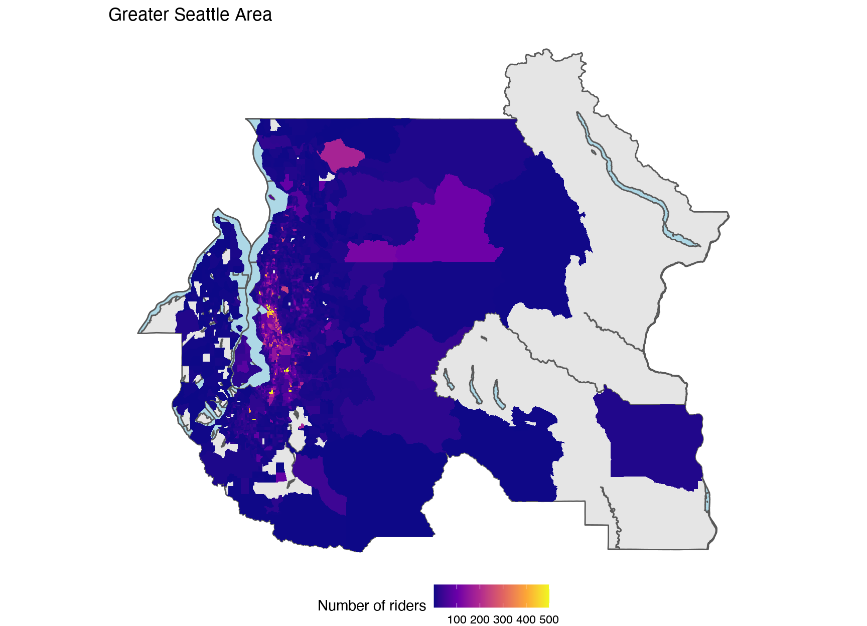
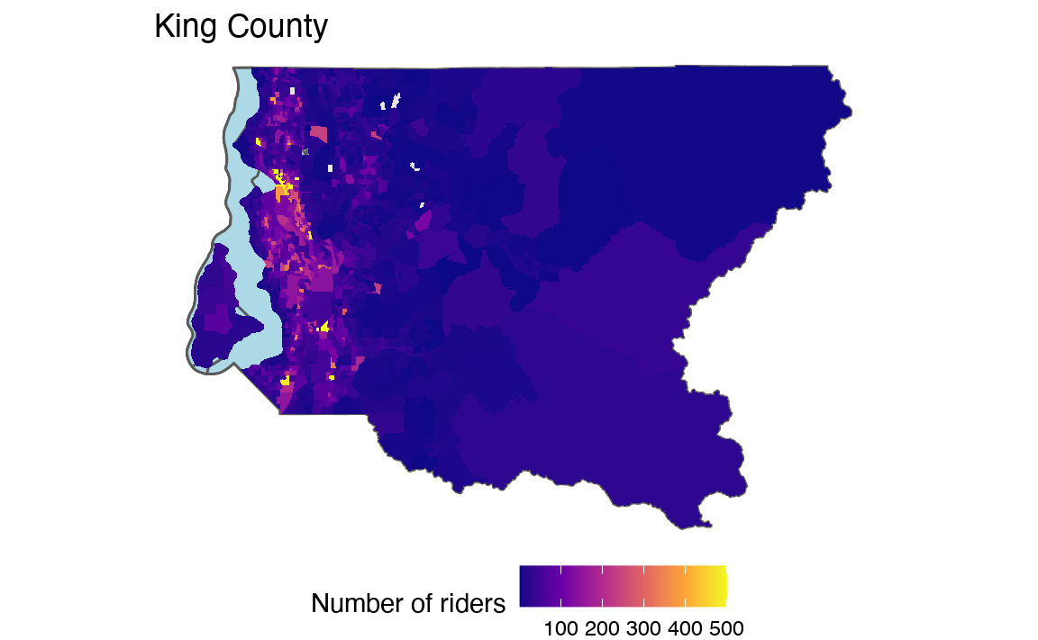
Plot rider count for fun

Code
# Filter the tigris data
county_shapes <- wa_counties %>% 
  filter(NAME %in% seattle_counties)

water_plot <- seattle_water %>% 
  filter(AWATER >= 1000000)

# Join the ACS data to the rider block groups
rider_bgs <- riders_final %>% 
  count(FIPS, name = "n_riders") %>% 
  left_join(acs_wa, by = c("FIPS" = "GEOID"))

# Join boundaries to observed rider block groups
geo_rider_bgs <- rider_bgs %>% 
  left_join(select(wa_bgs, GEOID, geometry), by = c("FIPS" = "GEOID")) %>% 
  st_sf() %>%   # Make the geometry column magical again
  # Truncate the number of riders
  mutate(n_riders_trunc = ifelse(n_riders >= 500, 500, n_riders))

# Plot
ggplot() +
  geom_sf(data = county_shapes, fill = "grey90") +
  geom_sf(data = water_plot, fill = "lightblue") +
  geom_sf(data = geo_rider_bgs, aes(fill = n_riders_trunc), size = 0) +
  scale_fill_viridis_c(option = "plasma") +
  labs(title = "Greater Seattle Area", fill = "Number of riders") +
  theme_void() +
  theme(legend.position = "bottom")

King County only

Code
kc_shape <- county_shapes %>% 
  filter(NAME == "King")

kc_water <- water_plot %>% 
  filter(county == "King")

kc_geo_rider <- geo_rider_bgs %>% 
  filter(str_starts(FIPS, "53033"))

ggplot() +
  geom_sf(data = kc_shape, fill = "grey90") +
  geom_sf(data = kc_water, fill = "lightblue") +
  geom_sf(data = kc_geo_rider, aes(fill = n_riders_trunc), size = 0) +
  scale_fill_viridis_c(option = "plasma") +
  labs(title = "King County", fill = "Number of riders") +
  theme_void() +
  theme(legend.position = "bottom")

Reenrollment patterns (see original)

The one year spike makes sense — re-enrollment needs to be done at the 1 year point. The spike at 0 might be cards with data entry errors.

Code
riders_who_reenroll <- riders_final %>% 
  filter(times > 1) %>% 
  distinct(id) %>% pull(id)

reenroll_timing <- riders_final %>% 
  filter(id %in% riders_who_reenroll) %>% 
  group_by(id) %>% 
  mutate(days_between = as.duration(interval(lag(DateIssued), DateIssued)) %/% as.duration(days(1)))

ggplot(reenroll_timing, aes(x = days_between)) +
  geom_histogram(binwidth = 7, boundary = 0) +
  geom_vline(xintercept = 0:5 * 365)