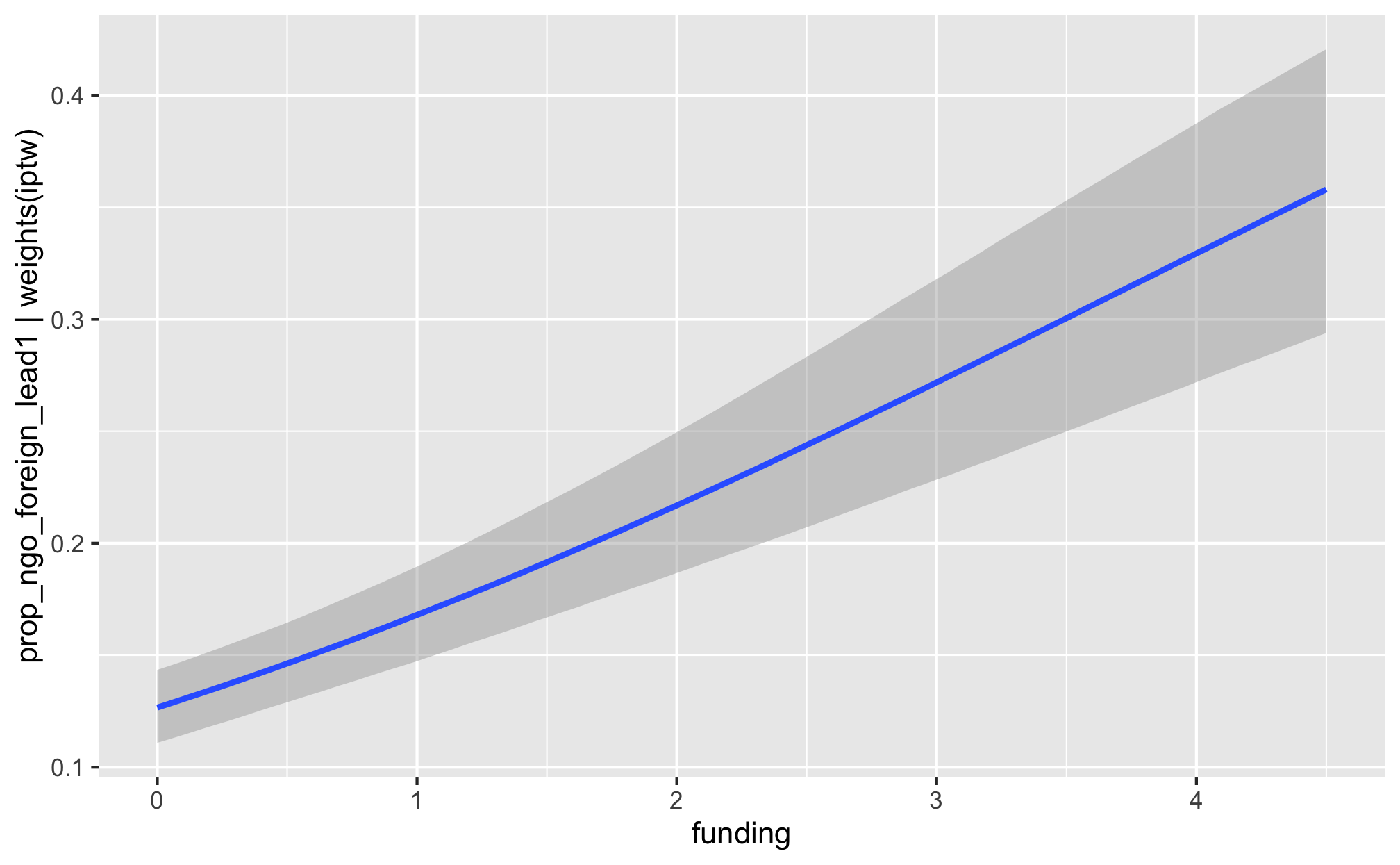
H₃: Effect of anti-NGO crackdown on aid recipients

library(tidyverse)
library(targets)
library(brms)
library(tidybayes)
library(bayesplot)
library(fixest)
library(broom)
library(broom.mixed)
library(modelsummary)
library(patchwork)
library(tictoc)
library(latex2exp)
library(scales)
library(extraDistr)
library(glue)
library(here)

color_scheme_set("viridisC")

labs_exp_logged <- function(brks) {TeX(paste0("e^{", as.character(log(brks)), "}"))}
labs_exp <- function(brks) {TeX(paste0("e^{", as.character(brks), "}"))}

my_seed <- 1234
set.seed(my_seed)

withr::with_dir(here::here(), {
  source(tar_read(plot_funs))
  source(tar_read(misc_funs))
  
  # Data
  df_country_aid <- tar_read(country_aid_final)
  df_country_aid_laws <- filter(df_country_aid, laws)
  
  # Models
  tar_load(c(m_recip_treatment_total_dom))
  tar_load(c(m_recip_outcome_total_dom, m_recip_outcome_total_foreign,
             m_recip_outcome_advocacy_dom, m_recip_outcome_advocacy_foreign,
             m_recip_outcome_entry_dom, m_recip_outcome_entry_foreign,
             m_recip_outcome_funding_dom, m_recip_outcome_funding_foreign))
})

Weight models

• Numerator is lagged treatment + non-varying confounders
• Denominator is lagged treatment + lagged outcome + time-varying confounders + non-varying confounders

\[ sw = \prod^t_{t = 1} \frac{\phi(T_{it} | T_{i, t-1}, C_i)}{\phi(T_{it} | T_{i, t-1}, D_{i, t-1}, C_i)} \]

Priors for weight models

We use generic weakly informative priors for our model parameters:

• Intercept: \(\mathcal{N} (0, 10)\)
• Coefficients: \(\mathcal{N} (0, 2.5)\)
• Sigma: \(\operatorname{Cauchy} (0, 1)\)

pri_int <- ggplot() +
  stat_function(fun = dnorm, args = list(mean = 0, sd = 10),
                geom = "area", fill = "grey80", color = "black") +
  labs(x = TeX("\\textbf{Intercept (β_0)}")) +
  annotate(geom = "label", x = 0, y = 0.01, label = "N(0, 10)", size = pts(9)) +
  xlim(-40, 40) +
  theme_donors(prior = TRUE)

pri_coef <- ggplot() +
  stat_function(fun = dnorm, args = list(mean = 0, sd = 2.5),
                geom = "area", fill = "grey80", color = "black") +
  labs(x = TeX("\\textbf{Coefficients (β_x)}")) +
  annotate(geom = "label", x = 0, y = 0.04, label = "N(0, 3)", size = pts(9)) +
  xlim(-10, 10) +
  theme_donors(prior = TRUE)

pri_sigma <- ggplot() +
  stat_function(fun = dcauchy, args = list(location = 0, scale = 1),
                geom = "area", fill = "grey80", color = "black") +
  labs(x = "σ") +
  annotate(geom = "label", x = 5, y = 0.08, label = "Cauchy(0, 1)", size = pts(9)) +
  xlim(0, 10) +
  theme_donors(prior = TRUE)

(pri_int + pri_coef + pri_sigma)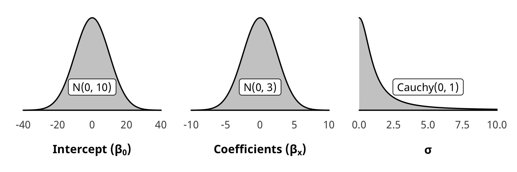

Check weight models

We check one of the denominator models for convergence and mixing and fit (not the numerator, since those models are the same as the ones in H1).

pp_check(m_recip_treatment_total_dom$model_denom, type = "dens_overlay", nsamples = 10) +
  theme_donors()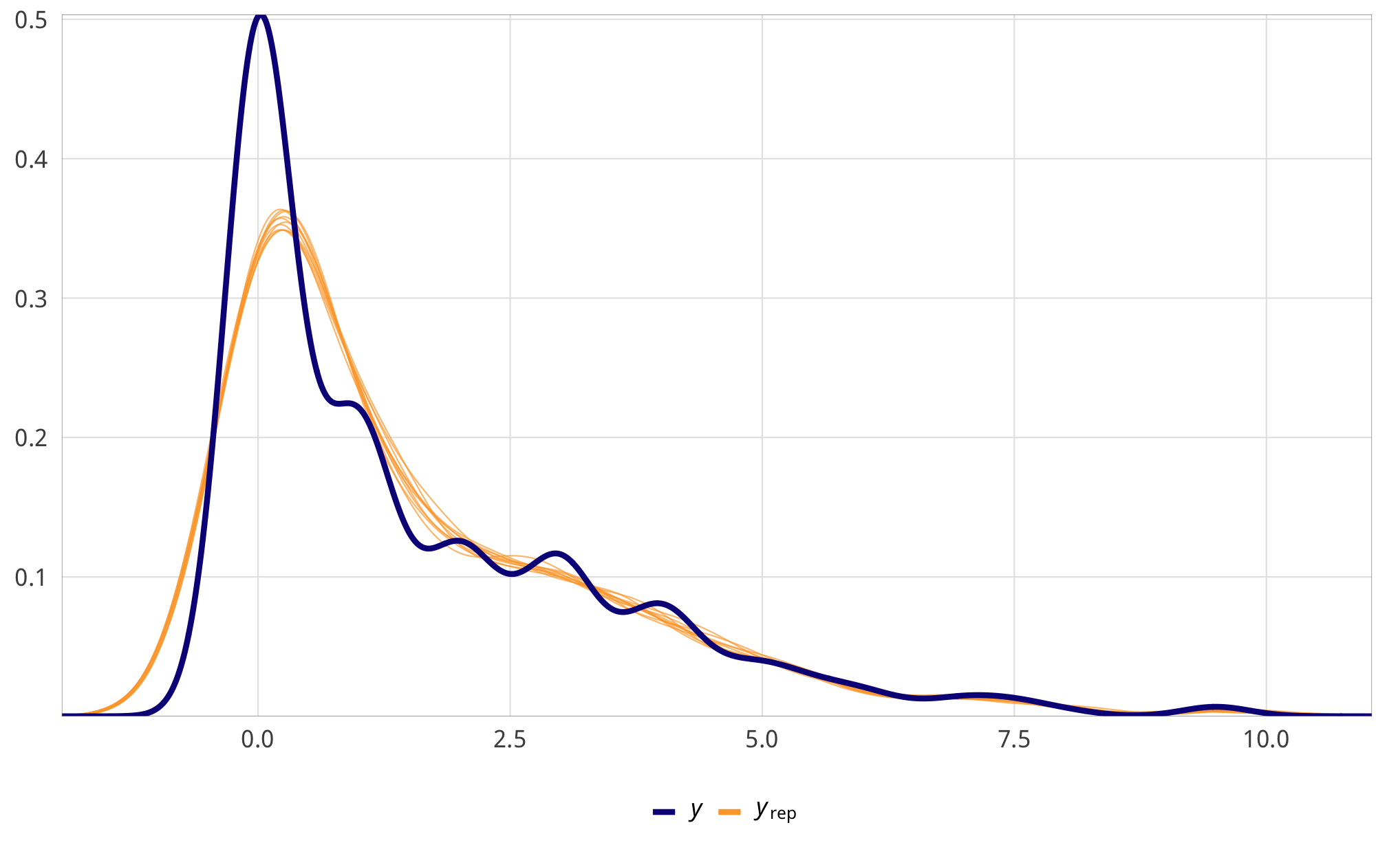

m_recip_treatment_total_dom$model_denom %>% 
  posterior_samples(add_chain = TRUE) %>% 
  select(-starts_with("r_gwcode"), -starts_with("z_"), -lp__, -iter) %>% 
  mcmc_trace() +
  theme_donors() +
  theme(legend.position = "right")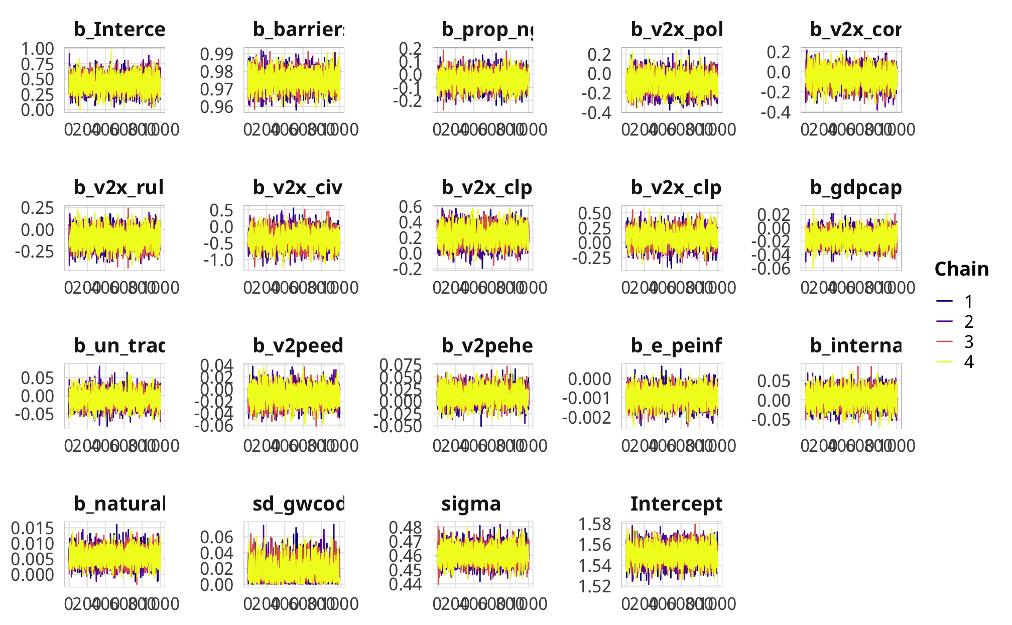

Outcome models

Modeling choice

We use two dependent variables for this hypothesis: the proportion of USAID aid channeled through either (1) domestic or (2) international or US-based (or foreign) NGOs, once again leaded by one year. The OECD and AidData do not track the channels of aid delivery, so we cannot see how aid is distributed on a global scale. USAID, however, does track channels, so we can measure how much aid goes to domestic NGOs (and also US-based and international NGOs). USAID didn’t start tracking this until 2001, though, so we have to limit our models to 2001–2013. (Boo.)

These variables are proportions and limited to a [0, 1] range. In the original version of this project, we used logit-linear models of the ratio of domestic or foriegn aid to all other channels, like this:

\[ln( \frac{\text{Aid to (domestic or foreign) NGOs}_{\text{USAID}}}{\text{Aid to other channels}_{\text{USAID}}} )_{i, t+1} = \text{NGO legislation}_{it} + \text{controls}_{it}\]

But as mentioned in our analysis for H₂, this made interpretation really strange. It also fails to account for zero- and one- inflation. These two variables have a lot of zeroes and a handful of ones, which indicates that there’s something highly systematic about the choice to (1) channel any money through any kind of NGOs and (2) how much money if so.

df_channels_plot_hist <- df_country_aid_laws %>% 
  pivot_longer(names_to = "channel", values_to = "value", 
               c(prop_ngo_dom, prop_ngo_foreign)) %>% 
  mutate(channel = recode(channel, 
                          prop_ngo_dom = "Domestic NGOs", 
                          prop_ngo_foreign = "Foreign NGOs"))

ggplot(df_channels_plot_hist, 
       aes(x = value, fill = channel, alpha = value == 0)) +
  geom_histogram(binwidth = 0.05, color = "white", boundary = 0) +
  labs(x = "Proportion of aid to NGOs", y = "Count") +
  scale_fill_manual(values = c("#001f3f", "#FF851B"), 
                    labels = c("Domestic", "International"),
                    name = NULL) +
  scale_alpha_manual(values = c(1, 0.5), 
                     labels = c("% > 0", "% = 0"),
                     name = NULL) +
  guides(fill = FALSE) +
  scale_x_continuous(labels = percent_format(accuracy = 1)) +
  facet_wrap(vars(channel)) +
  theme_donors()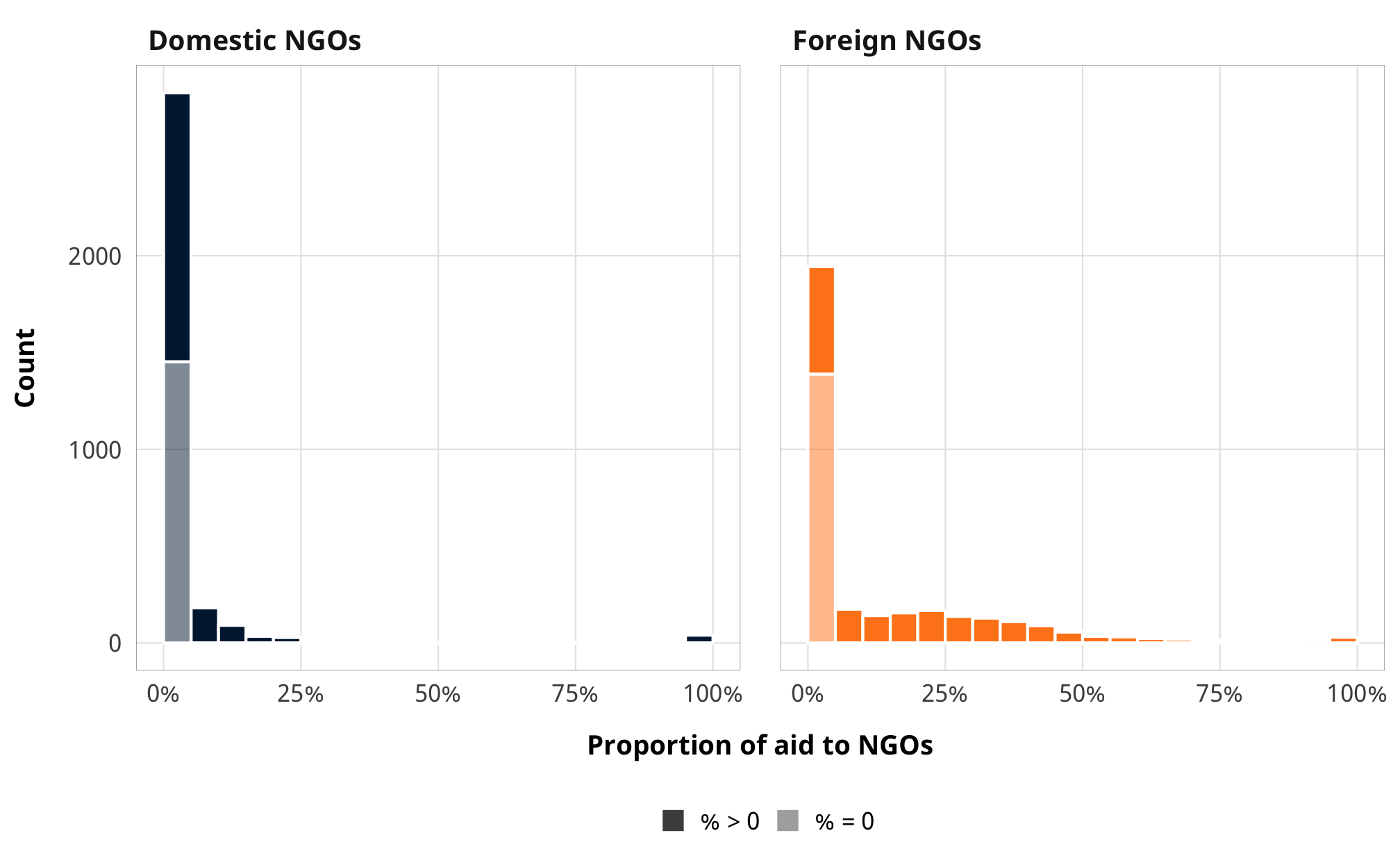

# Percent where prop_ngo_dom/foreign is 0:
df_channels_plot_hist %>% 
  count(channel, value == 0) %>% 
  group_by(channel) %>% 
  mutate(prop = n / sum(n))

## # A tibble: 4 x 4
## # Groups:   channel [2]
##   channel       `value == 0`     n  prop
##   <chr>         <lgl>        <int> <dbl>
## 1 Domestic NGOs FALSE         1841 0.559
## 2 Domestic NGOs TRUE          1452 0.441
## 3 Foreign NGOs  FALSE         1905 0.578
## 4 Foreign NGOs  TRUE          1388 0.422

Around 40% of observations are zero for both domestic and international NGOs, which is a lot (in H₂, ≈18% of rows had 0% contentious aid). Accordingly, it’s really important to model both the choice of whether to channel aid to NGOs and how much.

We thus use zero-inflated beta regression. We do not use zero-one-inflated regression because there are so few 1-only rows and we’re less interested in why a country would channel all its aid through NGOs (also, that’s more likely a sign of low aid to a country and just an artefact of the data generating process). We winsorize the few 1-only rows to 0.999.

As explained in H₂, zero-inflated beta models use a logit model to predict 0/not 0 and then use a beta family to model the rest of the data. In H₂ we were less interested in the mechanics of the zero-inflation process and modeled it with an intercept-only logit model. Here, though, given that there are so many 0s, we use the same confounders that we used in the weights model. We do not include inverse probability weights in the zero-inflation part because (1) the inner mechanics of brms don’t allow for that and (2) I’m not sure that works with marginal structural models anyway.

Priors for outcome models

Once again there are a ton of moving parts in these outcome models. Here’s the full specification for the models and all priors:

\[ \begin{aligned} \text{y}_{i,t} | u_i, \text{Law}_{i, t} &\sim \operatorname{ZIBeta} (Z_i, \text{y}^\star_i, \phi_i) & \text{[likelihood]} \\ \operatorname{logit} (Z_i) &\sim \alpha_Z & \text{[logit if } \text{y}_{i, t} = 0 \text{]} \\ \operatorname{logit} (\text{y}^\star_i) &\sim (\beta_0 + \beta_1 \text{Law}_{i, t} + \beta_2 \text{Law}_{i, t-1}, \sigma^2_\epsilon, u_i) \times \text{IPW}_{i, t} & \text{[if } \text{y}_{i, t} > 0 \text{]}\\ \log (\phi_i) &\sim \alpha_\phi & \text{[intercept-only model for precision]} \\ u_i &\sim \mathcal{N} (0, \sigma^2_u) & \text{[country-specific intercepts]} \\ \ \\ \alpha_Z &\sim \operatorname{Logistic}(-0.5, 0.35) & \text{[prior proportion of rows where y = 0]} \\ \alpha_\phi &\sim \operatorname{Gamma} (0.01, 0.01) & \text{[prior Beta precision]} \\ \beta_0 &\sim \mathcal{N} (0, 10) & \text{[prior population intercept]} \\ \beta_1, \beta_2 &\sim \mathcal{N} (0, 3) & \text{[prior population effects]} \\ \sigma^2_e, \sigma^2_u &\sim \operatorname{Cauchy}(0, 1) & \text{[prior sd for population and country]} \\ \ \\ \text{IPW}_{i, t} &= \prod^t_{t = 1} \frac{\phi(T_{it} | T_{i, t-1}, C_i)}{\phi(T_{it} | T_{i, t-1}, D_{i, t-1}, C_i)} & \text{[stabilized weights]} \end{aligned} \]

For \(\phi\), we just use Stan’s default Gamma(0.01, 0.01). Here’s what all these prior distributions look like:

z_p <- ggplot() +
  stat_function(fun = dlogis, args = list(location = -1.5, scale = 0.5),
                geom = "area", fill = "grey80", color = "black") +
  labs(x = TeX("\\textbf{Prop. contentious = 0 (α_Z)}")) +
  annotate(geom = "label", x = -2, y = 0.07, label = "Logistic(-1.5, 0.5)", size = pts(9)) +
  xlim(-8, 3) +
  theme_donors(prior = TRUE)

b0_p <- ggplot() +
  stat_function(fun = dnorm, args = list(mean = 0, sd = 10),
                geom = "area", fill = "grey80", color = "black") +
  labs(x = TeX("\\textbf{Population intercept (β_0)}")) +
  annotate(geom = "label", x = 0, y = 0.0042, label = "N(0, 10)", size = pts(9)) +
  xlim(-40, 40) +
  theme_donors(prior = TRUE)

b12_p <- ggplot() +
  stat_function(fun = dnorm, args = list(mean = 0, sd = 3),
                geom = "area", fill = "grey80", color = "black") +
  labs(x = TeX("\\textbf{Population effects (β_1, β_2)}")) +
  annotate(geom = "label", x = 0, y = 0.02, label = "N(0, 3)", size = pts(9)) +
  xlim(-10, 10) +
  theme_donors(prior = TRUE)

sigma_p <- ggplot() +
  stat_function(fun = dcauchy, args = list(location = 0, scale = 1),
                geom = "area", fill = "grey80", color = "black") +
  labs(x = TeX("\\textbf{Population and country SD (σ_e, σ_u)}")) +
  annotate(geom = "label", x = 5, y = 0.04, label = "Cauchy(0, 1)", size = pts(9)) +
  xlim(0, 10) +
  theme_donors(prior = TRUE)

phi_p <- ggplot() +
  stat_function(fun = dgamma, args = list(shape = 0.1, scale = 0.1),
                geom = "area", fill = "grey80", color = "black") +
  labs(x = TeX("\\textbf{Beta precision (φ)}")) +
  annotate(geom = "label", x = 0.25, y = 2, label = "Gamma(0.01, 0.01)", size = pts(9)) +
  xlim(0, 0.5) +
  theme_donors(prior = TRUE)

layout <- "
AAAABBBBCCCC
AAAABBBBCCCC
##DDDDEEEE##
##DDDDEEEE##
"
z_p + sigma_p + phi_p + b0_p + b12_p +
  plot_layout(design = layout)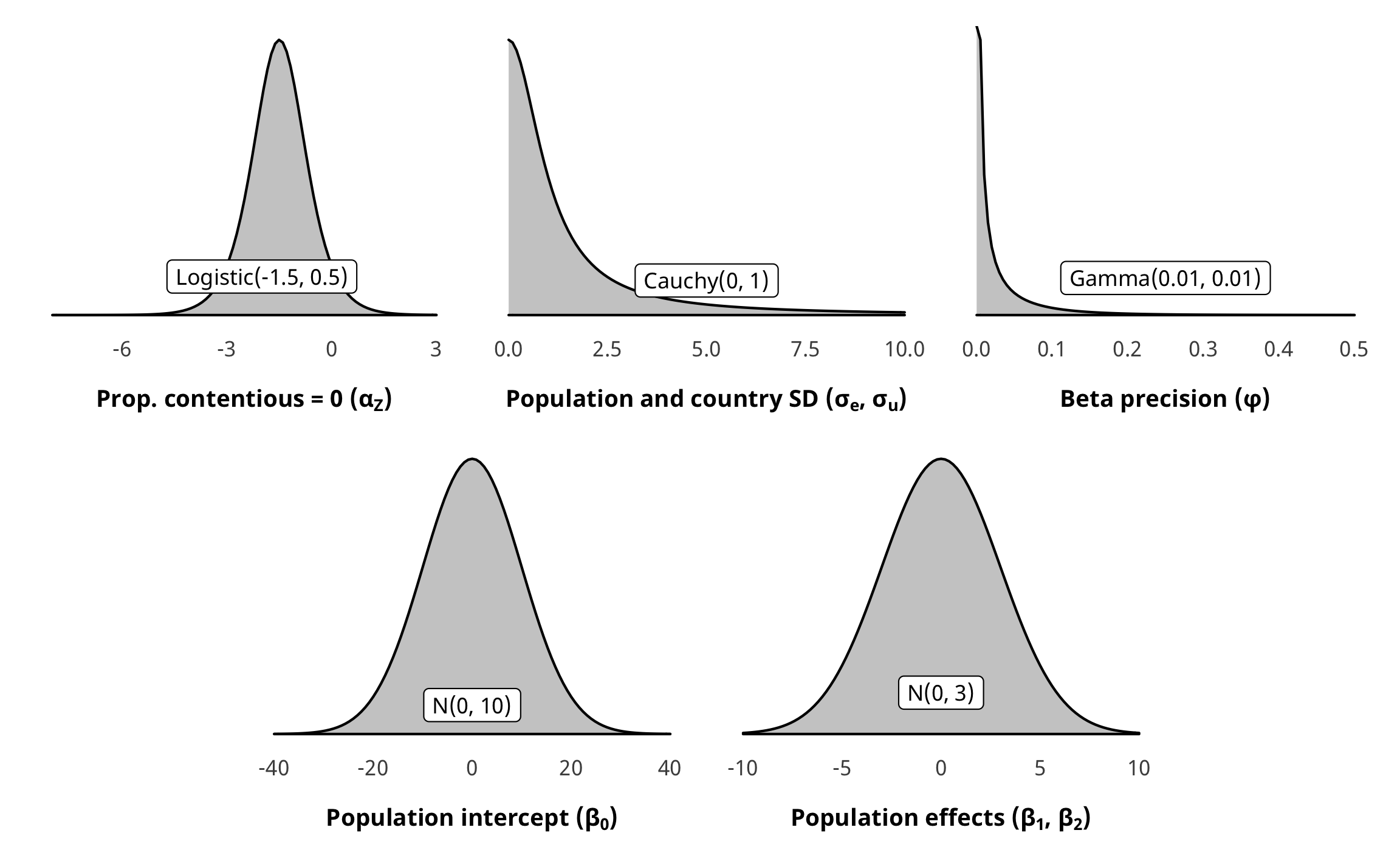

As with H₁ and H₂, the prior for the zero-inflated part of the model is a little weird. Internally, Stan uses a default of logistic(0, 1). We want to use an informative beta(8, 12) prior that approximates the proportion of zeroes in the data (but with fairly wide dispersion), but we once again need to translate it into the logistic distribution. Since there’s no easy way to do this, we used brms::logit_scaled to play around with distributional hyperparameters until it looked okay in the logistic distribution.

zi_prior_sim <- tibble(beta = rbeta(10000, 8, 12)) %>% 
  mutate(beta_logit_scale = brms::logit_scaled(beta)) %>% 
  mutate(logit_betaish_prior = rlogis(10000, -0.5, 0.35)) %>% 
  mutate(prior_probs = plogis(logit_betaish_prior))

zi_prior_plot1 <- ggplot(zi_prior_sim) +
  geom_density(aes(x = beta), fill = "grey80", color = "black") +
  labs(x = "Proportion where prop. contentious = 0",
       subtitle = "Original Beta(8, 12) distribution") +
  coord_cartesian(xlim = c(0, 1)) +
  theme_donors(prior = TRUE)

zi_prior_plot2 <- ggplot(zi_prior_sim) +
  geom_density(aes(x = beta_logit_scale), fill = "grey80", color = "black") +
  labs(x = "Logistic value where prop. contentious = 0",
       subtitle = "Beta(8, 12) scaled with brms::logit_scaled") +
  coord_cartesian(xlim = c(-4, 2)) +
  theme_donors(prior = TRUE)

zi_prior_plot3 <- ggplot(zi_prior_sim) +
  geom_density(aes(x = logit_betaish_prior), fill = "grey80", color = "black") +
  labs(x = "Logistic value where prop. contentious = 0",
       subtitle = "Estimated Logistic(-0.5, 0.35)") +
  coord_cartesian(xlim = c(-4, 2)) +
  theme_donors(prior = TRUE)

zi_prior_plot4 <- ggplot(zi_prior_sim) +
  geom_density(aes(x = prior_probs), fill = "grey80", color = "black") +
  labs(x = "Proportion where prop. contentious = 0",
       subtitle = "Logistic(-0.5, 0.35) transformed to probabilities") +
  coord_cartesian(xlim = c(0, 1)) +
  theme_donors(prior = TRUE)

(zi_prior_plot1 + zi_prior_plot2) / (zi_prior_plot3 + zi_prior_plot4)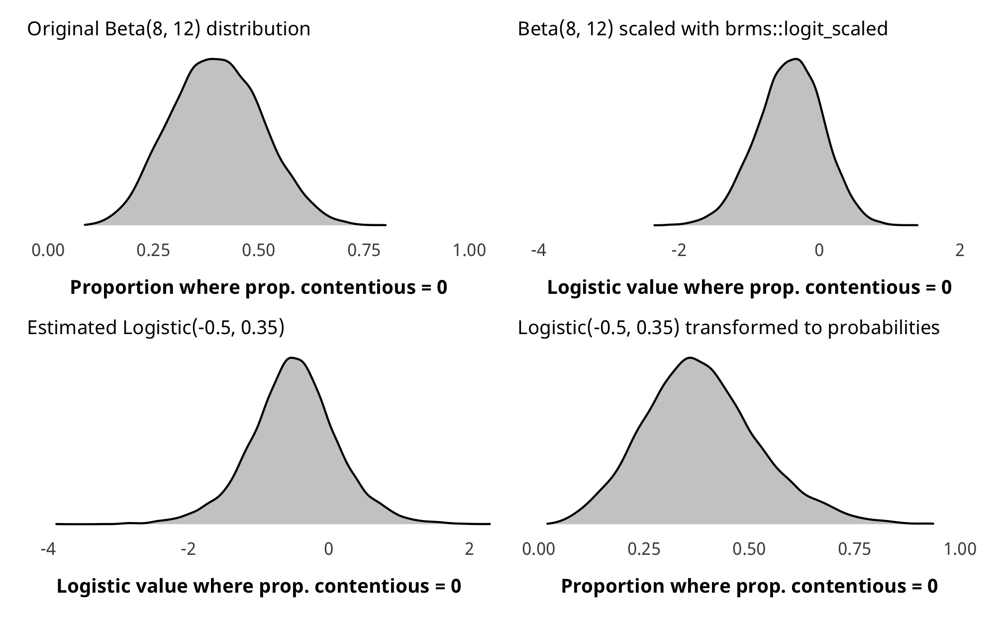

Check outcome models

pp_check(m_recip_outcome_total_dom, type = "dens_overlay", nsamples = 10) +
  scale_x_continuous(labels = percent_format(accuracy = 1)) +
  theme_donors()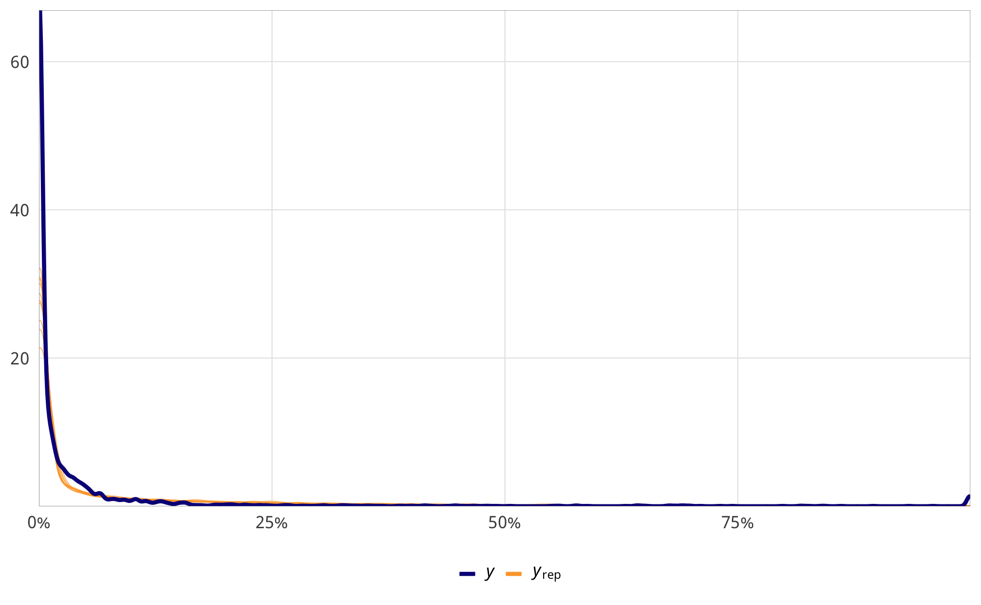

m_recip_outcome_total_dom %>% 
  posterior_samples(add_chain = TRUE) %>% 
  select(-starts_with("r_gwcode"), -starts_with("z_"), -lp__, -iter) %>% 
  mcmc_trace() +
  theme_donors()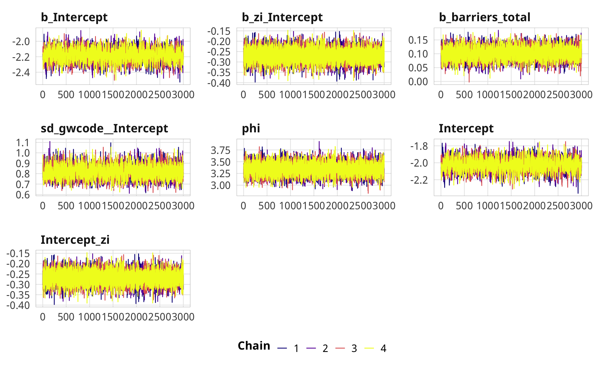

Results

# Plots!
plot_total_dom <- m_recip_outcome_total_dom %>% 
  gather_draws(b_barriers_total) %>%
  mutate(.value = exp(.value) - 1) %>% 
  mutate(.variable = dplyr::recode(.variable, 
                                   b_barriers_total = "Additional law, t - 1")) %>% 
  ggplot(aes(y = fct_rev(.variable), x = .value, fill = fct_rev(.variable))) +
  geom_vline(xintercept = 0) +
  stat_halfeye(.width = c(0.8, 0.95), alpha = 0.8) +
  guides(fill = FALSE) +
  scale_x_continuous(labels = percent_format(accuracy = 1)) +
  scale_fill_manual(values = c("#FF851B", "#FFDC00")) +
  labs(y = NULL, x = NULL) +
  theme_donors()

plot_total_foreign <- m_recip_outcome_total_foreign %>% 
  gather_draws(b_barriers_total) %>%
  mutate(.value = exp(.value) - 1) %>% 
  mutate(.variable = dplyr::recode(.variable, 
                                   b_barriers_total = "Additional law, t - 1")) %>% 
  ggplot(aes(y = fct_rev(.variable), x = .value, fill = fct_rev(.variable))) +
  geom_vline(xintercept = 0) +
  stat_halfeye(.width = c(0.8, 0.95), alpha = 0.8) +
  guides(fill = FALSE) +
  scale_x_continuous(labels = percent_format(accuracy = 1)) +
  scale_fill_manual(values = c("#FF851B", "#FFDC00")) +
  labs(y = NULL, x = NULL) +
  theme_donors()

plot_advocacy_dom <- m_recip_outcome_advocacy_dom %>% 
  gather_draws(b_advocacy) %>% 
  mutate(.variable = dplyr::recode(.variable, 
                                   b_advocacy = "Additional advocacy law, t - 1")) %>% 
  mutate(.value = exp(.value) - 1) %>% 
  ggplot(aes(y = fct_rev(.variable), x = .value, fill = fct_rev(.variable))) +
  geom_vline(xintercept = 0) +
  stat_halfeye(.width = c(0.8, 0.95), alpha = 0.8) +
  guides(fill = FALSE) +
  scale_x_continuous(labels = percent_format(accuracy = 1)) +
  scale_fill_manual(values = c("#85144b", "#F012BE")) +
  labs(y = NULL, x = NULL) +
  theme_donors()

plot_advocacy_foreign <- m_recip_outcome_advocacy_foreign %>% 
  gather_draws(b_advocacy) %>% 
  mutate(.variable = dplyr::recode(.variable, 
                                   b_advocacy = "Additional advocacy law, t - 1")) %>% 
  mutate(.value = exp(.value) - 1) %>% 
  ggplot(aes(y = fct_rev(.variable), x = .value, fill = fct_rev(.variable))) +
  geom_vline(xintercept = 0) +
  stat_halfeye(.width = c(0.8, 0.95), alpha = 0.8) +
  guides(fill = FALSE) +
  scale_x_continuous(labels = percent_format(accuracy = 1)) +
  scale_fill_manual(values = c("#85144b", "#F012BE")) +
  labs(y = NULL, x = NULL) +
  theme_donors()

plot_entry_dom <- m_recip_outcome_entry_dom %>% 
  gather_draws(b_entry) %>% 
  mutate(.variable = dplyr::recode(.variable, 
                                   b_entry = "Additional entry law, t - 1")) %>% 
  mutate(.value = exp(.value) - 1) %>% 
  ggplot(aes(y = fct_rev(.variable), x = .value, fill = fct_rev(.variable))) +
  geom_vline(xintercept = 0) +
  stat_halfeye(.width = c(0.8, 0.95), alpha = 0.8) +
  guides(fill = FALSE) +
  scale_x_continuous(labels = percent_format(accuracy = 1)) +
  scale_fill_manual(values = c("#3D9970", "#2ECC40")) +
  labs(y = NULL, x = "% change in proportion of aid to domestic NGOs") +
  theme_donors()

plot_entry_foreign <- m_recip_outcome_entry_foreign %>% 
  gather_draws(b_entry) %>% 
  mutate(.variable = dplyr::recode(.variable, 
                                   b_entry = "Additional entry law, t - 1")) %>% 
  mutate(.value = exp(.value) - 1) %>% 
  ggplot(aes(y = fct_rev(.variable), x = .value, fill = fct_rev(.variable))) +
  geom_vline(xintercept = 0) +
  stat_halfeye(.width = c(0.8, 0.95), alpha = 0.8) +
  guides(fill = FALSE) +
  scale_x_continuous(labels = percent_format(accuracy = 1)) +
  scale_fill_manual(values = c("#3D9970", "#2ECC40")) +
  labs(y = NULL, x = "% change in proportion of aid to foreign NGOs") +
  theme_donors()

plot_funding_dom <- m_recip_outcome_funding_dom %>% 
  gather_draws(b_funding) %>% 
  mutate(.variable = dplyr::recode(.variable, 
                                   b_funding = "Additional funding law, t - 1")) %>% 
  mutate(.value = exp(.value) - 1) %>% 
  ggplot(aes(y = fct_rev(.variable), x = .value, fill = fct_rev(.variable))) +
  geom_vline(xintercept = 0) +
  stat_halfeye(.width = c(0.8, 0.95), alpha = 0.8) +
  guides(fill = FALSE) +
  scale_x_continuous(labels = percent_format(accuracy = 1)) +
  scale_fill_manual(values = c("#001f3f", "#0074D9")) +
  labs(y = NULL, x = "% change in proportion aid to domestic NGOs") +
  theme_donors()

plot_funding_foreign <- m_recip_outcome_funding_foreign %>% 
  gather_draws(b_funding) %>% 
  mutate(.variable = dplyr::recode(.variable, 
                                   b_funding = "Additional funding law, t - 1")) %>% 
  mutate(.value = exp(.value) - 1) %>% 
  ggplot(aes(y = fct_rev(.variable), x = .value, fill = fct_rev(.variable))) +
  geom_vline(xintercept = 0) +
  stat_halfeye(.width = c(0.8, 0.95), alpha = 0.8) +
  guides(fill = FALSE) +
  scale_x_continuous(labels = percent_format(accuracy = 1)) +
  scale_fill_manual(values = c("#001f3f", "#0074D9")) +
  labs(y = NULL, x = "% change in proportion aid to foreign NGOs") +
  theme_donors()

(plot_total_dom + plot_advocacy_dom) / (plot_entry_dom + plot_funding_dom)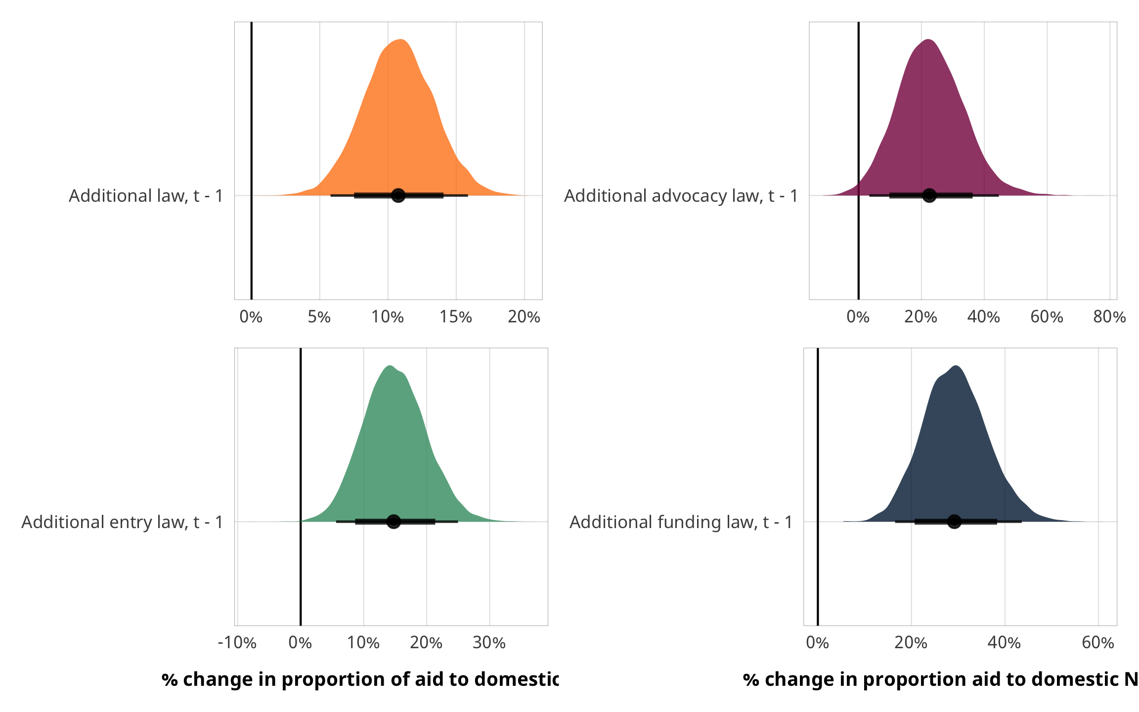

(plot_total_foreign + plot_advocacy_foreign) / (plot_entry_foreign + plot_funding_foreign)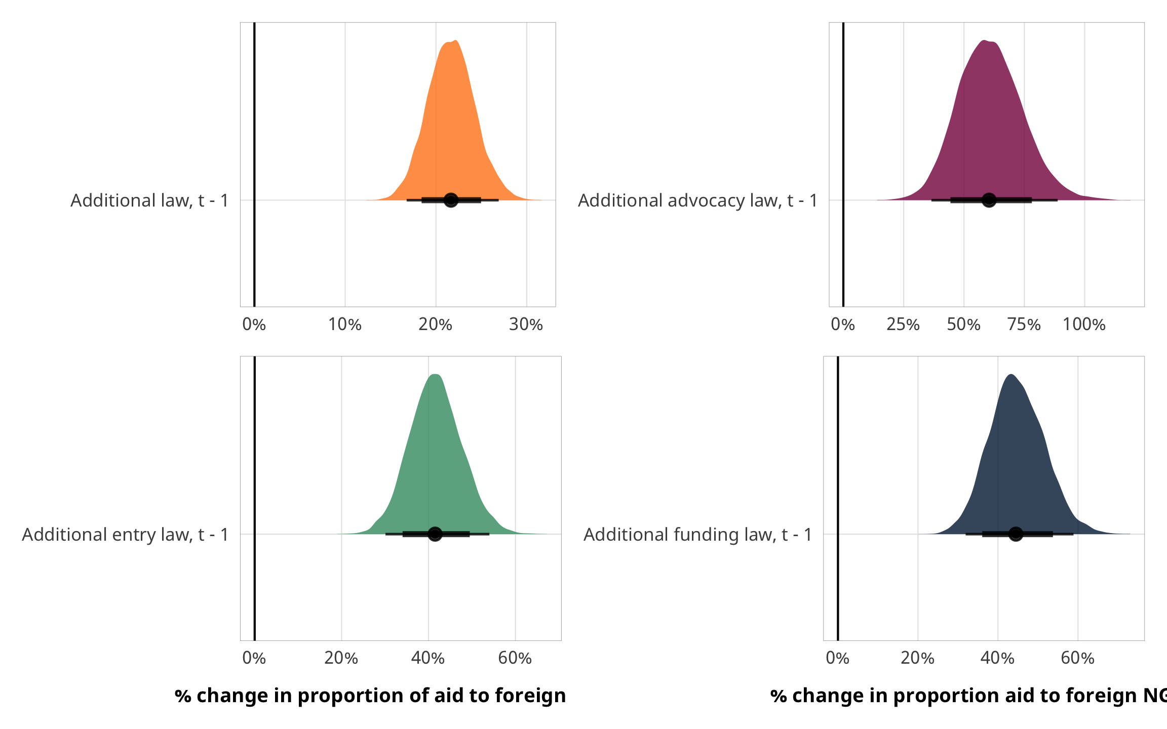

A one-unit change in X results in a relative change of \(e^\beta\) in \(\frac{\text{E(Proportion)}}{1 - \text{E(Proportion)}}\) - see https://stats.stackexchange.com/questions/297659/interpretation-of-betareg-coef - the ratio of contentious to non-contentious aid? the ratio of of contentious aid?

See also https://stats.stackexchange.com/a/230679/3025 and https://static1.squarespace.com/static/58a7d1e52994ca398697a621/t/5a2ebc43e4966b0fab6b02de/1513012293857/betareg_politics.pdf

m_recip_outcome_total_dom %>% 
  conditional_effects()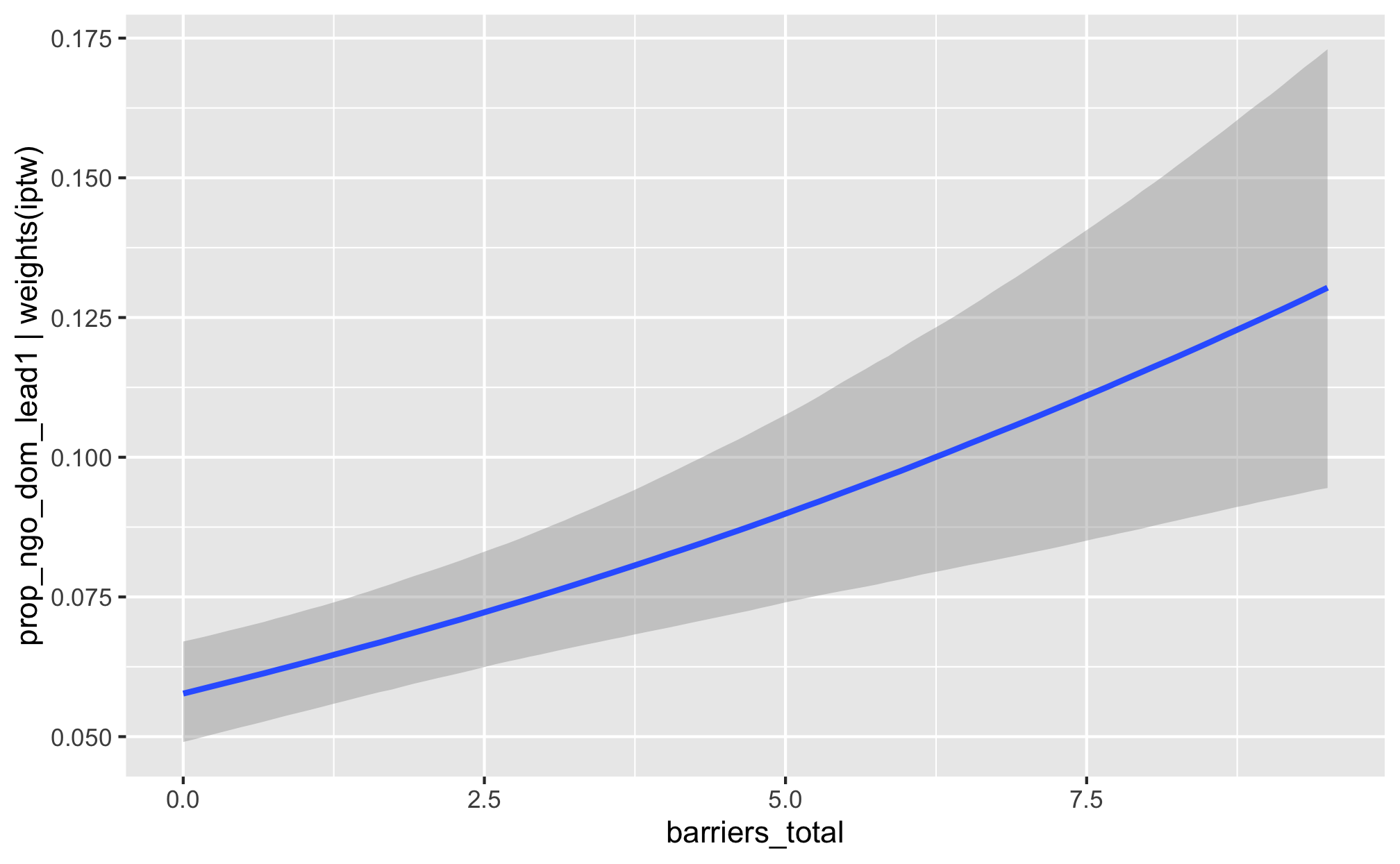

m_recip_outcome_advocacy_dom %>% 
  conditional_effects()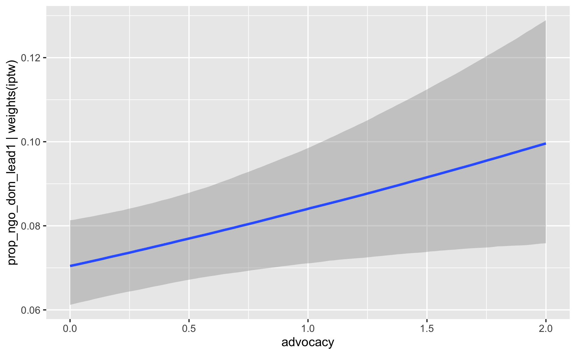

m_recip_outcome_entry_dom %>% 
  conditional_effects()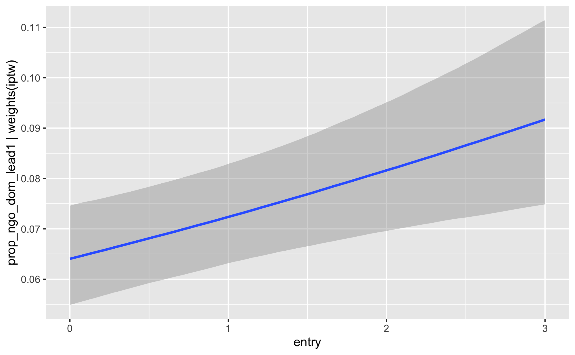

m_recip_outcome_funding_dom %>% 
  conditional_effects()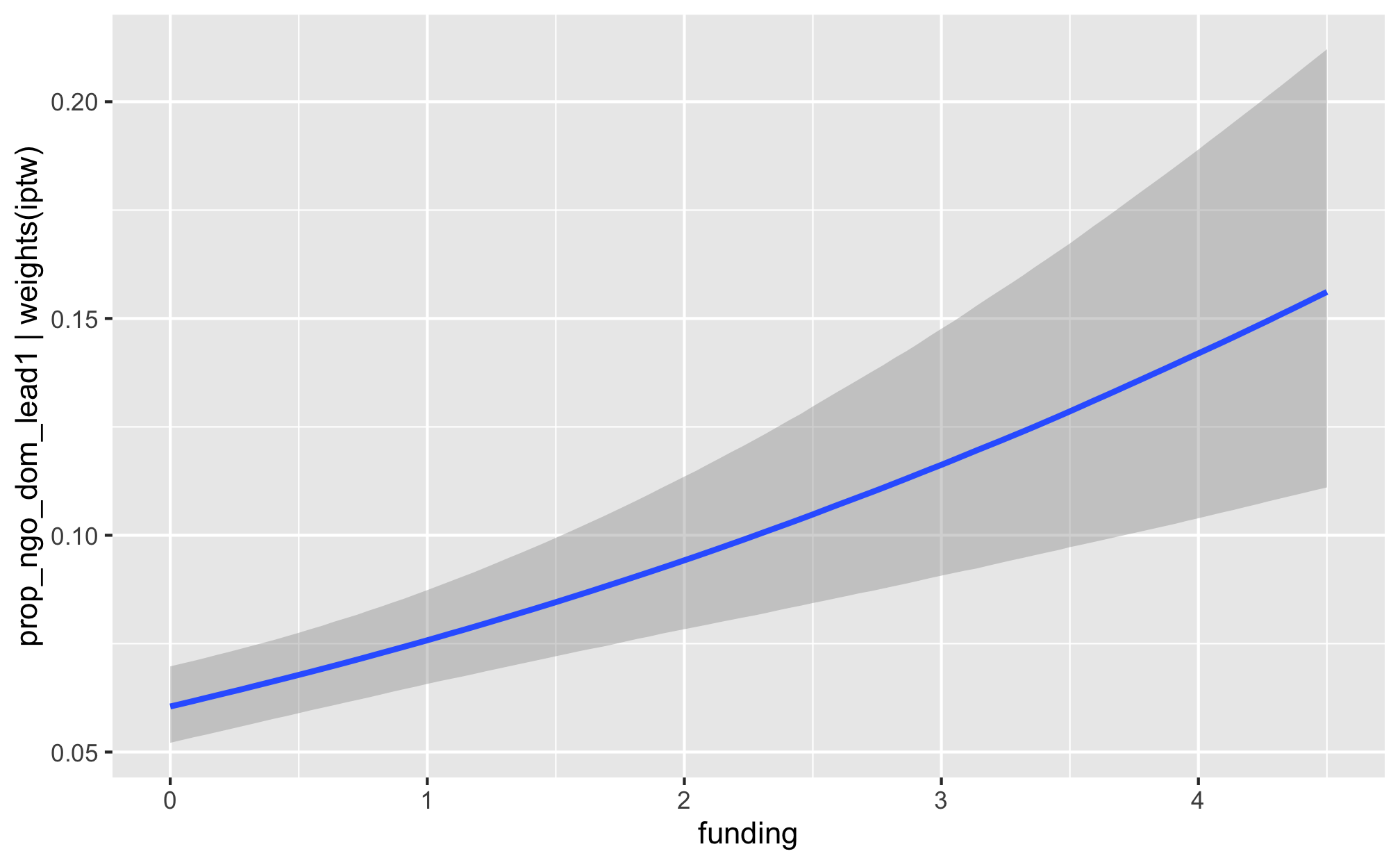

m_recip_outcome_total_foreign %>% 
  conditional_effects()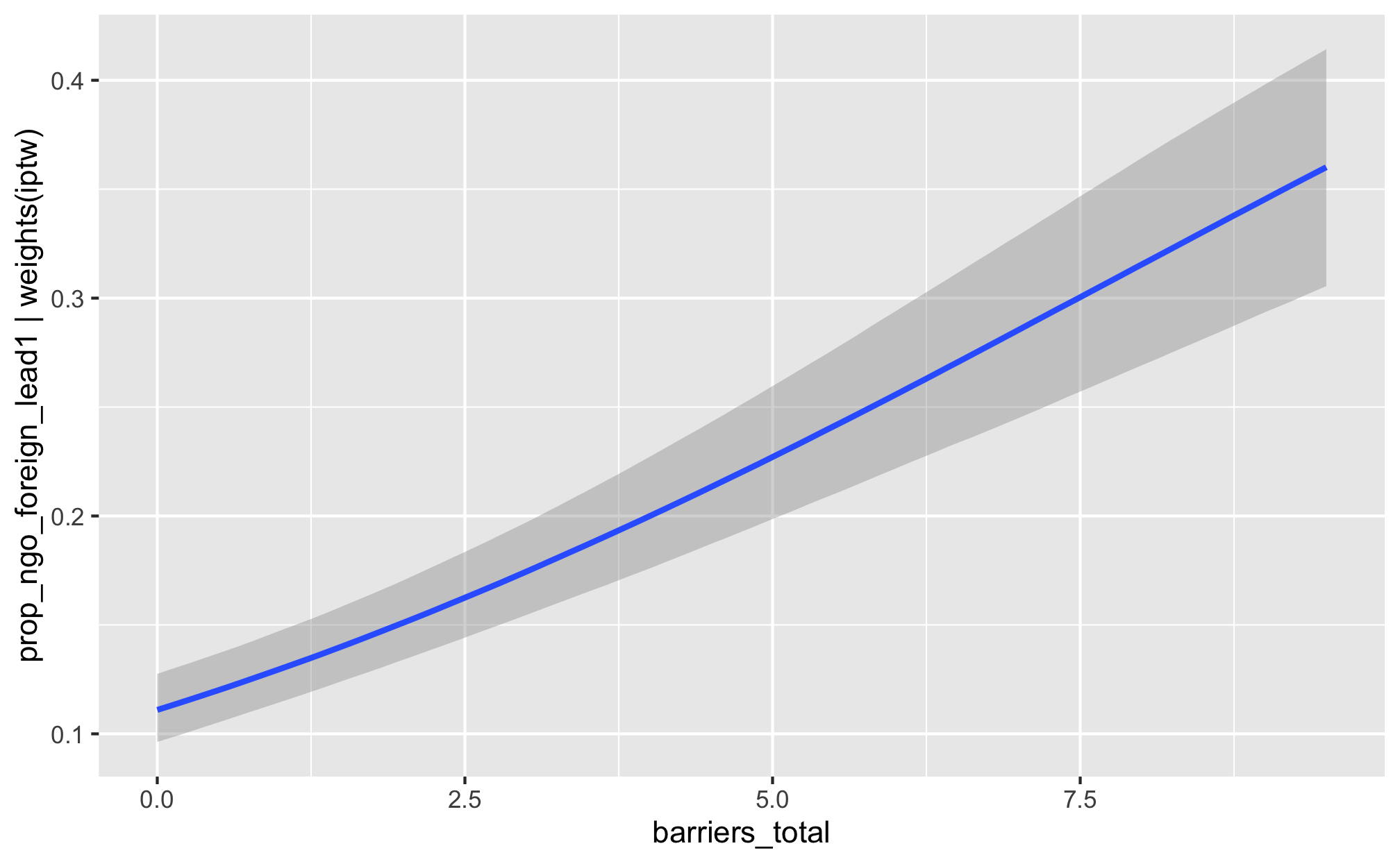

m_recip_outcome_advocacy_foreign %>% 
  conditional_effects()

m_recip_outcome_entry_foreign %>% 
  conditional_effects()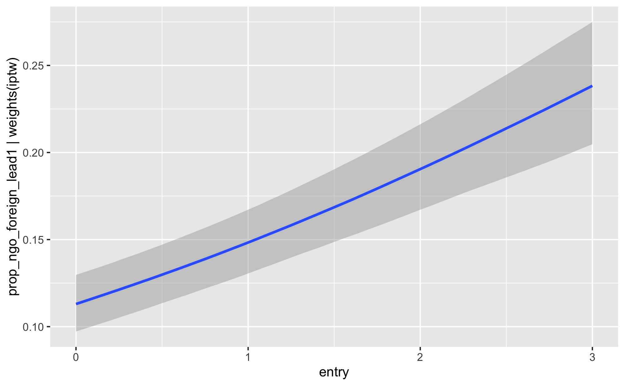

m_recip_outcome_funding_foreign %>% 
  conditional_effects()

Copyright © 2017–2021 Suparna Chaudhry and Andrew Heiss. Licensed under the MIT License. Code available on GitHub.