Process and merge data

library(tidyverse)
library(targets)
library(scales)
library(patchwork)
library(DT)
library(naniar)
library(here)

# Generated via random.org
set.seed(9936)

# Load data
# Need to use this withr thing because tar_read() and tar_load() need to see the
# _targets folder in the current directory, but this .Rmd file is in a subfolder
withr::with_dir(here::here(), {
  source(tar_read(plot_funs))
  
  tar_load(skeleton)
  tar_load(chaudhry_clean)
  tar_load(pts_clean)
  tar_load(latent_hr_clean)
  tar_load(vdem_clean)
  tar_load(wdi_clean)
  tar_load(un_pop)
  tar_load(un_gdp)
  tar_load(ucdp_prio_clean)
  
  tar_load(panel)
})

Data processing

Country-year skeleton

We use Gleditsch-Ward country codes to identify each country across the different datasets we merge. We omit a bunch of things though:

• We omit microstates
• Because the World Bank doesn’t include it in the WDI, we omit Taiwan (713)
• We only use countries in Suparna’s anti-NGO law data

To get consistency in country codes, we do this:

• When converting GW codes to COW codes, following Gleditsch and Ward, we treat post-2006 Serbia as 345 (a continuation of Serbia & Montenegro). And we also treat Serbia as a continuation of Yugoslavia with 345 (following V-Dem, which does that too)
• In both COW and GW codes, modern Vietnam is 816, but countrycode() thinks the COW code is 817, which is old South Vietnam (see issue), so we use custom_match to force 816 to recode to 816.
• Also, following V-Dem, we treat Czechoslovakia (GW/COW 315) and Czech Republic (GW/COW 316) as the same continuous country (V-Dem has both use ID 157).

We have 162 countries in this data, spanning 24 possible years. Here’s a lookup table of all the countries included:

skeleton$skeleton_lookup %>% 
  filter(gwcode %in% unique(chaudhry_clean$gwcode)) %>% 
  select(-years_included) %>% 
  datatable()

Chaudhry NGO restrictions

We create several indexes for each of the categories of regulation, following Christensen and Weinstein’s classification:

• entry (Q2b, Q2c, Q2d; 3 points maximum, actual max = 3 points maximum): barriers to entry
  • Q2c is reversed, so not being allowed to appeal registration status earns 1 point.
  • Q2a is omitted because it’s benign
• funding (Q3b, Q3c, Q3d, Q3e, Q3f; 5 points maximum, actual max = 4.5): barriers to funding
  • Q3a is omitted because it’s benign
  • Scores that range between 0–2 are rescaled to 0–1 (so 1 becomes 0.5)
• advocacy (Q4a, Q4c; 2 points maximum, actual max = 2): barriers to advocacy
  • Q4b is omitted because it’s not a law
  • Scores that range between 0–2 are rescaled to 0–1 (so 1 becomes 0.5)
• barriers_total (10 points maximum, actual max = 8.5): sum of all three indexes

These indexes are also standardized by dividing by the maximum, yielding the following variables:

• entry_std: 1 point maximum, actual max = 1
• funding_std: 1 point maximum, actual max = 1
• advocacy_std: 1 point maximum, actual max = 1
• barriers_total_std: 3 points maximum, actual max = 2.5

glimpse(chaudhry_clean)

## Rows: 3,965
## Columns: 22
## $ gwcode                         <dbl> 2, 2, 2, 2, 2, 2, 2, 2, 2, 2, 2, 2, 2, 2, 2, 2, 2…
## $ year                           <dbl> 1990, 1991, 1992, 1993, 1994, 1995, 1996, 1997, 1…
## $ advocacy                       <dbl> 0, 0, 0, 0, 0, 0, 0, 0, 0, 0, 0, 0, 0, 0, 0, 0, 0…
## $ entry                          <dbl> 1, 1, 1, 1, 1, 1, 1, 1, 1, 1, 1, 1, 1, 1, 1, 1, 1…
## $ funding                        <dbl> 0, 0, 0, 0, 0, 0, 0, 0, 0, 0, 0, 0, 0, 0, 0, 0, 0…
## $ entry_std                      <dbl> 0.3333333, 0.3333333, 0.3333333, 0.3333333, 0.333…
## $ funding_std                    <dbl> 0, 0, 0, 0, 0, 0, 0, 0, 0, 0, 0, 0, 0, 0, 0, 0, 0…
## $ advocacy_std                   <dbl> 0, 0, 0, 0, 0, 0, 0, 0, 0, 0, 0, 0, 0, 0, 0, 0, 0…
## $ barriers_total                 <dbl> 1, 1, 1, 1, 1, 1, 1, 1, 1, 1, 1, 1, 1, 1, 1, 1, 1…
## $ barriers_total_std             <dbl> 0.3333333, 0.3333333, 0.3333333, 0.3333333, 0.333…
## $ ngo_register                   <dbl> 0, 0, 0, 0, 0, 0, 0, 0, 0, 0, 0, 0, 0, 0, 0, 0, 0…
## $ ngo_register_burden            <dbl> 0, 0, 0, 0, 0, 0, 0, 0, 0, 0, 0, 0, 0, 0, 0, 0, 0…
## $ ngo_register_appeal            <dbl> 0, 0, 0, 0, 0, 0, 0, 0, 0, 0, 0, 0, 0, 0, 0, 0, 0…
## $ ngo_barrier_foreign_funds      <dbl> 1, 1, 1, 1, 1, 1, 1, 1, 1, 1, 1, 1, 1, 1, 1, 1, 1…
## $ ngo_disclose_funds             <dbl> 1, 1, 1, 1, 1, 1, 1, 1, 1, 1, 1, 1, 1, 1, 1, 1, 1…
## $ ngo_foreign_fund_approval      <dbl> 0, 0, 0, 0, 0, 0, 0, 0, 0, 0, 0, 0, 0, 0, 0, 0, 0…
## $ ngo_foreign_fund_channel       <dbl> 0, 0, 0, 0, 0, 0, 0, 0, 0, 0, 0, 0, 0, 0, 0, 0, 0…
## $ ngo_foreign_fund_restrict      <dbl> 0, 0, 0, 0, 0, 0, 0, 0, 0, 0, 0, 0, 0, 0, 0, 0, 0…
## $ ngo_foreign_fund_prohibit      <dbl> 0, 0, 0, 0, 0, 0, 0, 0, 0, 0, 0, 0, 0, 0, 0, 0, 0…
## $ ngo_type_foreign_fund_prohibit <dbl> 0, 0, 0, 0, 0, 0, 0, 0, 0, 0, 0, 0, 0, 0, 0, 0, 0…
## $ ngo_politics                   <dbl> 0, 0, 0, 0, 0, 0, 0, 0, 0, 0, 0, 0, 0, 0, 0, 0, 0…
## $ ngo_politics_foreign_fund      <dbl> 0, 0, 0, 0, 0, 0, 0, 0, 0, 0, 0, 0, 0, 0, 0, 0, 0…

Political Terror Scale (PTS)

We use data from the Political Terror Scale (PTS) project to measure state repression. This project uses reports from the US State Department, Amnesty International, and Human Rights Watch and codes political repression on a scale of 1-5:

• Level 1: Countries under a secure rule of law, people are not imprisoned for their view, and torture is rare or exceptional. Political murders are extremely rare.
• Level 2: There is a limited amount of imprisonment for nonviolent political activity. However, few persons are affected, torture and beatings are exceptional. Political murder is rare.
• Level 3: There is extensive political imprisonment, or a recent history of such imprisonment. Execution or other political murders and brutality may be common. Unlimited detention, with or without a trial, for political views is accepted.
• Level 4: Civil and political rights violations have expanded to large numbers of the population. Murders, disappearances, and torture are a common part of life. In spite of its generality, on this level terror affects primarily those who interest themselves in politics or ideas.
• Level 5: The terrors of Level 4 have been extended to the whole population. The leaders of these societies place no limits on the means or thoroughness with which they pursue personal or ideological goals.

Following Gohdes and Carey, we use the State Department score, unless it’s missing, in which case we use Amnesty’s score.

glimpse(pts_clean)

## Rows: 7,564
## Columns: 4
## $ year       <int> 1976, 1977, 1978, 1979, 1980, 1981, 1982, 1983, 1984, 1985, 1986, 198…
## $ gwcode     <dbl> 700, 700, 700, 700, 700, 700, 700, 700, 700, 700, 700, 700, 700, 700,…
## $ PTS        <int> 2, 2, 3, 5, 5, 5, 5, 5, 5, 5, 5, 5, 5, 5, 4, 5, 5, 5, 5, 5, 5, 5, 5, …
## $ PTS_factor <ord> Level 2, Level 2, Level 3, Level 5, Level 5, Level 5, Level 5, Level …

Latent Human Rights Protection Scores

We also use Chris Fariss’s Latent Human Rights Protection Scores, which are estimates from fancy Bayesian models that capture a country’s respect for physical integrity rights. We use the posterior mean of the latent variable from the model (θ), and we keep the standard deviation of θ just in case we want to fancier things in the future and incorporate the uncertainty of θ in the models. We rename θ to latent_hr_mean.

In this measure, high values represent strong respect for physical integrity rights:

latent_hr_clean %>% 
  filter(latent_hr_mean == max(latent_hr_mean) | 
           latent_hr_mean == min(latent_hr_mean)) %>% 
  left_join(select(skeleton$skeleton_lookup, gwcode, country),
            by = "gwcode") %>% 
  select(country, everything())

country	year	gwcode	latent_hr_mean	latent_hr_sd
Luxembourg	2014	212	5.336182	1.1818222
Rwanda	1994	517	-3.391152	0.1950997

glimpse(latent_hr_clean)

## Rows: 5,021
## Columns: 4
## $ year           <dbl> 1990, 1991, 1992, 1993, 1994, 1995, 1996, 1997, 1998, 1999, 2000,…
## $ gwcode         <dbl> 2, 2, 2, 2, 2, 2, 2, 2, 2, 2, 2, 2, 2, 2, 2, 2, 2, 2, 2, 2, 2, 2,…
## $ latent_hr_mean <dbl> 1.545246803, 1.334556330, 1.295854765, 1.411467052, 1.477233396, …
## $ latent_hr_sd   <dbl> 0.2982614, 0.2877736, 0.2864317, 0.2909148, 0.2809583, 0.2817655,…

Varieties of Democracy (V-Dem)

We use a bunch of variables from the Varieties of Democracy project:

• Civil society stuff
  • CSO entry and exit: v2cseeorgs
  • CSO repression: v2csreprss
  • CSO consultation: v2cscnsult
  • CSO participatory environment: v2csprtcpt
  • CSO women’s participation: v2csgender
  • CSO anti-system movements: v2csantimv
  • Core civil society index (entry/exit, repression, participatory env): v2xcs_ccsi
• Freedom of expression stuff
  • Freedom of expression index: v2x_freexp
  • Freedom of expression and alternative sources of information index: v2x_freexp_altinf
  • Freedom of academic and cultural expression: v2clacfree
  • Media self-censorship: v2meslfcen
• Repression stuff
  • Religious organization repression: v2csrlgrep
  • Govt censorship effort - media: v2mecenefm
  • Harassment of journalists: v2meharjrn
• Rights indexes
  • Civil liberties index: v2x_civlib
  • Physical violence index: v2x_clphy
  • Private civil liberties index: v2x_clpriv
  • Political civil liberties index: v2x_clpol
• Democracy and governance stuff
  • Polyarchy index (for electoral democracies): v2x_polyarchy
  • Liberal democracy index (for democracies in general): v2x_libdem
  • Regimes of the world category: v2x_regime
  • Political corruption index: v2x_corr (less to more, 0-1) (public sector + executive + legislative + judicial corruption)
  • Rule of law index: v2x_rule

glimpse(vdem_clean)

## Rows: 5,206
## Columns: 25
## $ year              <dbl> 1990, 1991, 1992, 1993, 1994, 1995, 1996, 1997, 1998, 1999, 20…
## $ v2cseeorgs        <dbl> 0.187, 0.187, 0.187, 0.187, 0.187, 0.187, 0.187, 0.394, 0.394,…
## $ v2csreprss        <dbl> -0.641, -0.625, -0.625, -0.625, -0.415, -0.415, -0.415, -0.298…
## $ v2cscnsult        <dbl> 0.128, 0.128, 0.128, 0.128, 0.128, 0.353, 0.353, 0.876, 0.876,…
## $ v2csprtcpt        <dbl> -0.693, -0.693, -0.693, -0.693, -0.353, 0.048, 0.048, 0.048, 0…
## $ v2csgender        <dbl> 0.453, 0.453, 0.453, 0.453, 0.703, 0.703, 0.703, 0.703, 0.703,…
## $ v2csantimv        <dbl> -0.879, -0.879, -0.879, -0.879, -0.879, -0.879, -0.879, -0.879…
## $ v2xcs_ccsi        <dbl> 0.410, 0.389, 0.389, 0.389, 0.406, 0.431, 0.431, 0.520, 0.616,…
## $ v2x_freexp        <dbl> 0.688, 0.688, 0.688, 0.746, 0.771, 0.766, 0.766, 0.766, 0.766,…
## $ v2x_freexp_altinf <dbl> 0.595, 0.636, 0.636, 0.637, 0.682, 0.686, 0.686, 0.686, 0.686,…
## $ v2clacfree        <dbl> 1.831, 1.831, 1.831, 1.831, 1.945, 1.949, 1.949, 1.949, 1.949,…
## $ v2meslfcen        <dbl> 0.493, 0.493, 0.493, 1.278, 1.278, 1.278, 1.278, 1.278, 1.278,…
## $ v2csrlgrep        <dbl> 0.020, 0.216, 0.216, 0.692, 0.692, 0.692, 0.692, 0.692, 0.692,…
## $ v2mecenefm        <dbl> 0.186, 0.186, 0.186, 0.186, 0.186, 0.186, 0.186, 0.186, 0.186,…
## $ v2meharjrn        <dbl> 0.625, 0.625, 0.625, 0.625, 0.625, 0.625, 0.625, 0.625, 0.625,…
## $ v2x_civlib        <dbl> 0.632, 0.605, 0.643, 0.642, 0.669, 0.696, 0.696, 0.686, 0.705,…
## $ v2x_clphy         <dbl> 0.454, 0.483, 0.483, 0.483, 0.483, 0.521, 0.521, 0.521, 0.521,…
## $ v2x_clpriv        <dbl> 0.715, 0.714, 0.762, 0.730, 0.785, 0.785, 0.785, 0.785, 0.785,…
## $ v2x_clpol         <dbl> 0.678, 0.657, 0.657, 0.682, 0.726, 0.722, 0.722, 0.725, 0.747,…
## $ v2x_polyarchy     <dbl> 0.389, 0.435, 0.448, 0.438, 0.482, 0.514, 0.528, 0.546, 0.596,…
## $ v2x_libdem        <dbl> 0.206, 0.221, 0.226, 0.222, 0.281, 0.295, 0.308, 0.336, 0.371,…
## $ v2x_regime        <dbl> 1, 1, 1, 1, 1, 2, 2, 2, 2, 2, 2, 2, 2, 2, 2, 2, 2, 2, 2, 2, 2,…
## $ v2x_corr          <dbl> 0.778, 0.778, 0.778, 0.778, 0.694, 0.678, 0.678, 0.665, 0.662,…
## $ v2x_rule          <dbl> 0.361, 0.361, 0.361, 0.361, 0.484, 0.523, 0.523, 0.544, 0.544,…
## $ gwcode            <dbl> 70, 70, 70, 70, 70, 70, 70, 70, 70, 70, 70, 70, 70, 70, 70, 70…

World Bank development indicators

We don’t really use anything from the World Bank’s data except for population data for Kosovo.

glimpse(wdi_clean)

## Rows: 4,930
## Columns: 6
## $ country    <chr> "United Arab Emirates", "United Arab Emirates", "United Arab Emirates…
## $ gwcode     <dbl> 696, 696, 696, 696, 696, 696, 696, 696, 696, 696, 696, 696, 696, 696,…
## $ year       <int> 1996, 1997, 1998, 1991, 1992, 1993, 1990, 1995, 2009, 2010, 1994, 199…
## $ region     <chr> "Middle East & North Africa", "Middle East & North Africa", "Middle E…
## $ income     <chr> "High income", "High income", "High income", "High income", "High inc…
## $ population <dbl> 2539121, 2671361, 2813214, 1937159, 2052892, 2173135, 1828437, 241509…

UNData

The reason we don’t just use WDI data for GDP and % of GDP from trade is that the WDI data is incomplete (especially pre-1990, but that’s not an issue in this project) To get around that, we create our own GDP and trade measures using data directly from the UN (at UNData). They don’t have a neat API like the World Bank, so you have to go to their website and export the data manually.

We collect three variables: GDP at constant 2015 prices, GDP at current prices, and population.

glimpse(un_pop)

## Rows: 12,010
## Columns: 3
## $ gwcode     <dbl> 516, 516, 516, 516, 516, 516, 516, 516, 516, 516, 516, 516, 516, 516,…
## $ year       <int> 1950, 1951, 1952, 1953, 1954, 1955, 1956, 1957, 1958, 1959, 1960, 196…
## $ population <dbl> 2308927, 2360442, 2406034, 2449089, 2492192, 2537150, 2584913, 263562…

glimpse(un_gdp)

## Rows: 7,812
## Columns: 4
## $ gwcode           <int> 700, 700, 700, 700, 700, 700, 700, 700, 700, 700, 700, 700, 700…
## $ year             <dbl> 2018, 2017, 2016, 2015, 2014, 2013, 2012, 2011, 2010, 2009, 200…
## $ un_trade_pct_gdp <dbl> 0.5097236, 0.5840631, 0.5431432, 0.5534622, 0.5090126, 0.544231…
## $ un_gdp           <dbl> 22485098073, 22865408739, 21341550985, 20608090681, 20983941434…

UCDP/PRIO Armed Conflict

Following Gohdes and Carey (2017), we use UCDP/PRIO Armed Conflict data to create an indicator marking if a country-year was involved in armed conflict that resulted in at least 25 battle-related deaths.

glimpse(ucdp_prio_clean)

## Rows: 1,695
## Columns: 3
## $ gwcode         <int> 2, 2, 2, 2, 2, 2, 2, 2, 2, 2, 2, 2, 2, 2, 2, 2, 2, 2, 40, 40, 40,…
## $ year           <dbl> 1950, 2001, 2002, 2003, 2004, 2005, 2006, 2007, 2008, 2009, 2010,…
## $ armed_conflict <lgl> TRUE, TRUE, TRUE, TRUE, TRUE, TRUE, TRUE, TRUE, TRUE, TRUE, TRUE,…

Final clean combined data

Finally, we join everything together in one nice clean panel:

glimpse(panel)

## Rows: 3,794
## Columns: 65
## $ gwcode                         <dbl> 2, 2, 2, 2, 2, 2, 2, 2, 2, 2, 2, 2, 2, 2, 2, 2, 2…
## $ year                           <dbl> 1990, 1991, 1992, 1993, 1994, 1995, 1996, 1997, 1…
## $ cowcode                        <dbl> 2, 2, 2, 2, 2, 2, 2, 2, 2, 2, 2, 2, 2, 2, 2, 2, 2…
## $ country                        <chr> "United States", "United States", "United States"…
## $ iso2                           <chr> "US", "US", "US", "US", "US", "US", "US", "US", "…
## $ iso3                           <chr> "USA", "USA", "USA", "USA", "USA", "USA", "USA", …
## $ un                             <dbl> 840, 840, 840, 840, 840, 840, 840, 840, 840, 840,…
## $ un_trade_pct_gdp               <dbl> 0.1981507, 0.1978645, 0.1995059, 0.2004462, 0.210…
## $ un_gdp                         <dbl> 9.807263e+12, 9.796646e+12, 1.014173e+13, 1.04209…
## $ population                     <dbl> 252120309, 254539371, 256990608, 259532130, 26224…
## $ gdpcap                         <dbl> 38899.14, 38487.74, 39463.42, 40152.69, 41338.87,…
## $ gdp_log                        <dbl> 29.91414, 29.91306, 29.94768, 29.97484, 30.01433,…
## $ gdpcap_log                     <dbl> 10.56873, 10.55810, 10.58313, 10.60044, 10.62956,…
## $ population_log                 <dbl> 19.34542, 19.35497, 19.36455, 19.37439, 19.38478,…
## $ advocacy                       <dbl> 0, 0, 0, 0, 0, 0, 0, 0, 0, 0, 0, 0, 0, 0, 0, 0, 0…
## $ entry                          <dbl> 1, 1, 1, 1, 1, 1, 1, 1, 1, 1, 1, 1, 1, 1, 1, 1, 1…
## $ funding                        <dbl> 0, 0, 0, 0, 0, 0, 0, 0, 0, 0, 0, 0, 0, 0, 0, 0, 0…
## $ entry_std                      <dbl> 0.3333333, 0.3333333, 0.3333333, 0.3333333, 0.333…
## $ funding_std                    <dbl> 0, 0, 0, 0, 0, 0, 0, 0, 0, 0, 0, 0, 0, 0, 0, 0, 0…
## $ advocacy_std                   <dbl> 0, 0, 0, 0, 0, 0, 0, 0, 0, 0, 0, 0, 0, 0, 0, 0, 0…
## $ barriers_total                 <dbl> 1, 1, 1, 1, 1, 1, 1, 1, 1, 1, 1, 1, 1, 1, 1, 1, 1…
## $ barriers_total_std             <dbl> 0.3333333, 0.3333333, 0.3333333, 0.3333333, 0.333…
## $ ngo_register                   <dbl> 0, 0, 0, 0, 0, 0, 0, 0, 0, 0, 0, 0, 0, 0, 0, 0, 0…
## $ ngo_register_burden            <dbl> 0, 0, 0, 0, 0, 0, 0, 0, 0, 0, 0, 0, 0, 0, 0, 0, 0…
## $ ngo_register_appeal            <dbl> 0, 0, 0, 0, 0, 0, 0, 0, 0, 0, 0, 0, 0, 0, 0, 0, 0…
## $ ngo_barrier_foreign_funds      <dbl> 1, 1, 1, 1, 1, 1, 1, 1, 1, 1, 1, 1, 1, 1, 1, 1, 1…
## $ ngo_disclose_funds             <dbl> 1, 1, 1, 1, 1, 1, 1, 1, 1, 1, 1, 1, 1, 1, 1, 1, 1…
## $ ngo_foreign_fund_approval      <dbl> 0, 0, 0, 0, 0, 0, 0, 0, 0, 0, 0, 0, 0, 0, 0, 0, 0…
## $ ngo_foreign_fund_channel       <dbl> 0, 0, 0, 0, 0, 0, 0, 0, 0, 0, 0, 0, 0, 0, 0, 0, 0…
## $ ngo_foreign_fund_restrict      <dbl> 0, 0, 0, 0, 0, 0, 0, 0, 0, 0, 0, 0, 0, 0, 0, 0, 0…
## $ ngo_foreign_fund_prohibit      <dbl> 0, 0, 0, 0, 0, 0, 0, 0, 0, 0, 0, 0, 0, 0, 0, 0, 0…
## $ ngo_type_foreign_fund_prohibit <dbl> 0, 0, 0, 0, 0, 0, 0, 0, 0, 0, 0, 0, 0, 0, 0, 0, 0…
## $ ngo_politics                   <dbl> 0, 0, 0, 0, 0, 0, 0, 0, 0, 0, 0, 0, 0, 0, 0, 0, 0…
## $ ngo_politics_foreign_fund      <dbl> 0, 0, 0, 0, 0, 0, 0, 0, 0, 0, 0, 0, 0, 0, 0, 0, 0…
## $ laws                           <lgl> TRUE, TRUE, TRUE, TRUE, TRUE, TRUE, TRUE, TRUE, T…
## $ PTS                            <int> 1, 2, 2, 1, 1, 1, 1, 1, 1, 1, 1, 2, 2, 2, 3, 3, 3…
## $ PTS_factor                     <ord> Level 1, Level 2, Level 2, Level 1, Level 1, Leve…
## $ latent_hr_mean                 <dbl> 1.54524680, 1.33455633, 1.29585476, 1.41146705, 1…
## $ latent_hr_sd                   <dbl> 0.2982614, 0.2877736, 0.2864317, 0.2909148, 0.280…
## $ v2cseeorgs                     <dbl> 2.622, 2.622, 2.622, 2.622, 2.622, 2.622, 2.622, …
## $ v2csreprss                     <dbl> 2.723, 2.723, 2.723, 2.723, 2.723, 2.723, 2.723, …
## $ v2cscnsult                     <dbl> 2.700, 2.700, 2.700, 2.700, 2.700, 2.700, 2.700, …
## $ v2csprtcpt                     <dbl> 2.900, 2.900, 2.900, 2.900, 2.900, 2.900, 2.900, …
## $ v2csgender                     <dbl> 1.542, 1.542, 1.542, 1.542, 1.542, 1.542, 1.542, …
## $ v2csantimv                     <dbl> -2.661, -2.661, -2.661, -2.661, -2.661, -2.661, -…
## $ v2xcs_ccsi                     <dbl> 0.964, 0.964, 0.964, 0.964, 0.964, 0.964, 0.964, …
## $ v2x_freexp                     <dbl> 0.969, 0.966, 0.967, 0.967, 0.967, 0.967, 0.967, …
## $ v2x_freexp_altinf              <dbl> 0.954, 0.949, 0.957, 0.945, 0.945, 0.945, 0.945, …
## $ v2clacfree                     <dbl> 3.085, 3.085, 3.085, 3.085, 3.085, 3.085, 3.085, …
## $ v2meslfcen                     <dbl> 2.603, 2.603, 2.603, 2.603, 2.603, 2.603, 2.603, …
## $ v2csrlgrep                     <dbl> 2.124, 2.124, 2.124, 2.124, 2.124, 2.124, 2.124, …
## $ v2mecenefm                     <dbl> 2.479, 1.517, 2.458, 2.458, 2.458, 2.458, 2.458, …
## $ v2meharjrn                     <dbl> 2.260, 2.260, 2.260, 2.260, 2.260, 2.260, 2.260, …
## $ v2x_civlib                     <dbl> 0.945, 0.946, 0.945, 0.945, 0.945, 0.945, 0.945, …
## $ v2x_clphy                      <dbl> 0.923, 0.923, 0.923, 0.923, 0.923, 0.923, 0.923, …
## $ v2x_clpriv                     <dbl> 0.942, 0.942, 0.942, 0.942, 0.942, 0.942, 0.942, …
## $ v2x_clpol                      <dbl> 0.973, 0.970, 0.976, 0.976, 0.976, 0.976, 0.976, …
## $ v2x_polyarchy                  <dbl> 0.873, 0.872, 0.873, 0.854, 0.858, 0.883, 0.881, …
## $ v2x_libdem                     <dbl> 0.802, 0.806, 0.809, 0.784, 0.793, 0.817, 0.816, …
## $ v2x_regime                     <dbl> 3, 3, 3, 3, 3, 3, 3, 3, 3, 3, 3, 3, 3, 3, 3, 3, 3…
## $ v2x_corr                       <dbl> 0.056, 0.056, 0.056, 0.056, 0.056, 0.056, 0.053, …
## $ v2x_rule                       <dbl> 0.978, 0.978, 0.978, 0.976, 0.975, 0.975, 0.982, …
## $ armed_conflict                 <lgl> FALSE, FALSE, FALSE, FALSE, FALSE, FALSE, FALSE, …
## $ armed_conflict_num             <dbl> 0, 0, 0, 0, 0, 0, 0, 0, 0, 0, 0, 1, 1, 1, 1, 1, 1…
## $ pred_group                     <chr> "Training", "Training", "Training", "Training", "…

 

Basic data details

panel %>% 
  summarize(`Number of countries` = length(unique(gwcode)),
            `Number of years` = length(unique(year)),
            `First year` = min(year),
            `Last year` = max(year)) %>% 
  kbl(align = "c") %>% 
  kable_styling()

Number of countries	Number of years	First year	Last year
162	24	1990	2013

Countries across years:

panel %>% 
  count(Year = year, name = "Number of countries") %>% 
  kbl(align = "c") %>% 
  kable_styling()

Year	Number of countries
1990	138
1991	153
1992	156
1993	158
1994	158
1995	158
1996	158
1997	158
1998	158
1999	158
2000	158
2001	158
2002	159
2003	159
2004	159
2005	159
2006	160
2007	160
2008	161
2009	161
2010	161
2011	162
2012	162
2013	162

 

Missingness

We were super careful to ensure that our data is as complete as possible.

panel %>% 
  vis_miss() +
  theme_ngo() +
  theme(axis.text.x = element_text(hjust = 0, angle = 45),
        panel.grid.major = element_blank())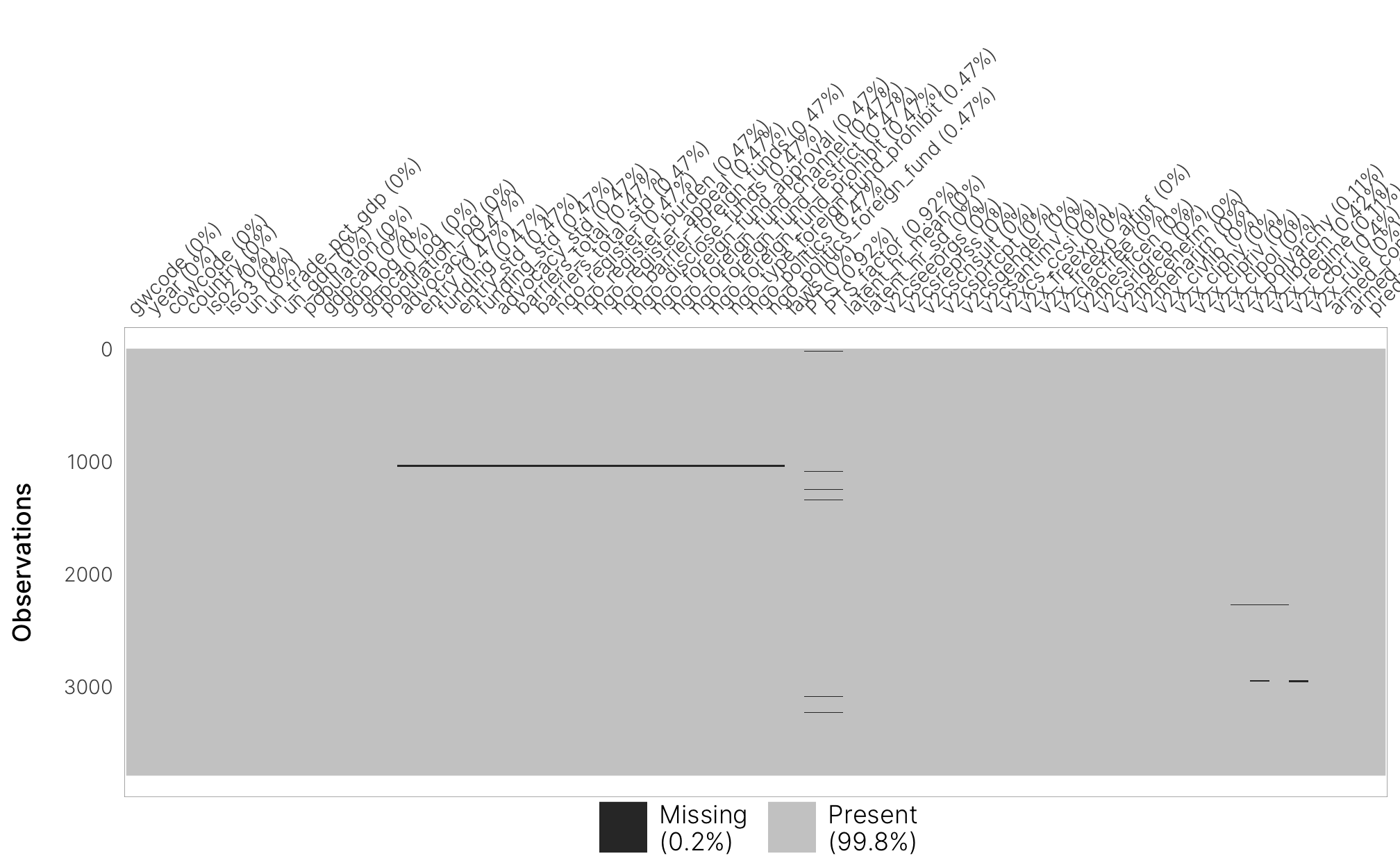

There are only a tiny handful of rows with missing NGO law data: Serbia pre-2006 and Russia pre-1992

panel %>% 
  filter(is.na(advocacy)) %>% 
  select(gwcode, year, country, iso3, advocacy, entry, funding)

gwcode	year	country	iso3	advocacy	entry	funding
345	1990	Serbia	SRB
345	1991	Serbia	SRB
345	1992	Serbia	SRB
345	1993	Serbia	SRB
345	1994	Serbia	SRB
345	1995	Serbia	SRB
345	1996	Serbia	SRB
345	1997	Serbia	SRB
345	1998	Serbia	SRB
345	1999	Serbia	SRB
345	2000	Serbia	SRB
345	2001	Serbia	SRB
345	2002	Serbia	SRB
345	2003	Serbia	SRB
345	2004	Serbia	SRB
345	2005	Serbia	SRB
365	1990	Russia	RUS
365	1991	Russia	RUS

That’s because our anti-NGO data doesn’t include data for those years. That’s fine, though. In models where we look at anti-NGO laws, we exclude those rows and only include rows where our laws indicator variable is TRUE. In models where we look at the general civil society environment, we do include these rows because V-Dem has data for them.

There are a handful of instances of missing data with PTS scores:

panel %>% 
  filter(is.na(PTS)) %>% 
  select(gwcode, year, country, iso3, PTS, PTS_factor)

gwcode	year	country	iso3	PTS	PTS_factor
2	2013	United States	USA
316	1990	Czechia	CZE
316	1991	Czechia	CZE
341	2007	Montenegro	MNE
343	1991	North Macedonia	MKD
345	1990	Serbia	SRB
349	1992	Slovenia	SVN
349	1993	Slovenia	SVN
349	1994	Slovenia	SVN
349	1995	Slovenia	SVN
349	1996	Slovenia	SVN
359	1991	Moldova	MDA
365	1990	Russia	RUS
365	1991	Russia	RUS
366	1991	Estonia	EST
367	1991	Latvia	LVA
368	1991	Lithuania	LTU
369	1991	Ukraine	UKR
370	1991	Belarus	BLR
371	1991	Armenia	ARM
372	1991	Georgia	GEO
373	1991	Azerbaijan	AZE
698	1992	Oman	OMN
701	1991	Turkmenistan	TKM
702	1991	Tajikistan	TJK
703	1991	Kyrgyzstan	KGZ
704	1991	Uzbekistan	UZB
705	1991	Kazakhstan	KAZ
731	1990	North Korea	PRK
731	1991	North Korea	PRK
731	1992	North Korea	PRK
731	1993	North Korea	PRK
731	1994	North Korea	PRK
731	1995	North Korea	PRK
731	1996	North Korea	PRK

We just ignore them, I guess.

With that, here’s our actual final cleaned data:

panel %>% 
  filter(laws) %>% 
  vis_miss() +
  theme_ngo() +
  theme(axis.text.x = element_text(hjust = 0, angle = 45),
        panel.grid.major = element_blank())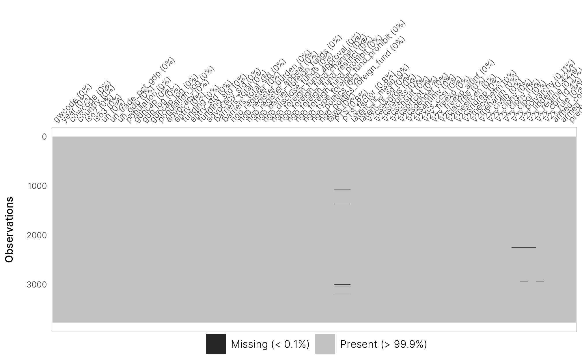

Beautiful.

 

targets pipeline

Here’s the general process for building and running this analysis. This is all done with the magical targets package, which orchestrates all the dependencies automatically.

 

Actual code

All the data processing is handled with dataset-specific functions that live in R/funs_data-cleaning.R, which targets then runs as needed. For the sake of transparency, here’s that code:

library(scales)
library(countrycode)
library(readxl)
library(haven)
library(jsonlite)
suppressPackageStartupMessages(library(sf))

# The PTS data is saved as an .RData file, so it loads into R with its original
# object name. This function lets you load an .RData file directly to a new
# object instead of bringing in the original name. (via
# https://stackoverflow.com/a/25455968/120898)
load_rdata <- function(filename) {
  load(filename)
  get(ls()[ls() != "filename"])
}


create_panel_skeleton <- function() {
  library(states)

  microstates <- gwstates %>%
    filter(microstate) %>% distinct(gwcode)

  # In both COW and GW codes, modern Vietnam is 816, but countrycode() thinks the
  # COW code is 817, which is old South Vietnam (see issue
  # https://github.com/vincentarelbundock/countrycode/issues/16), so we use
  # custom_match to force 816 to recode to 816
  #
  # Also, following Gleditsch and Ward, we treat Serbia after 2006 dissolution of
  # Serbia & Montenegro as 345 in COW codes (see
  # https://www.andybeger.com/states/articles/differences-gw-cow.html)
  #
  # Following V-Dem, we treat Czechoslovakia (GW/COW 315) and Czech Republic
  # (GW/COW 316) as the same continuous country (V-Dem has both use ID 157).
  #
  # Also, because the World Bank doesn't include it in the WDI, we omit
  # Taiwan (713). We also omit East Germany (265) and South Yemen (680).

  panel_skeleton <- state_panel(1990, 2014, partial = "any") %>%
    # Remove microstates
    filter(!(gwcode %in% microstates$gwcode)) %>%
    # Deal with Czechia
    mutate(gwcode = recode(gwcode, `315` = 316L)) %>%
    # Remove East Germany, South Yemen, Taiwan, the Bahamas, Belize, and Brunei
    filter(!(gwcode %in% c(265, 680, 713, 31, 80, 835))) %>%
    mutate(cowcode = countrycode(gwcode, origin = "gwn", destination = "cown",
                                 custom_match = c("816" = 816L, "340" = 345L)),
           country = countrycode(cowcode, origin = "cown", destination = "country.name",
                                 custom_match = c("678" = "Yemen")),
           iso2 = countrycode(cowcode, origin = "cown", destination = "iso2c",
                              custom_match = c("345" = "RS", "347" = "XK", "678" = "YE")),
           iso3 = countrycode(cowcode, origin = "cown", destination = "iso3c",
                              custom_match = c("345" = "SRB", "347" = "XKK", "678" = "YEM")),
           # Use 999 as the UN country code for Kosovo
           un = countrycode(cowcode, origin = "cown", destination = "un",
                            custom_match = c("345" = 688, "347" = 999, "678" = 887))) %>%
    # There are two entries for "Yugoslavia" in 2006 after recoding 340 as 345;
    # get rid of one
    filter(!(gwcode == 340 & cowcode == 345 & year == 2006)) %>%
    # Make Serbia 345 in GW codes too, for joining with other datasets
    mutate(gwcode = recode(gwcode, `340` = 345L)) %>%
    mutate(country = recode(country, `Yugoslavia` = "Serbia")) %>%
    arrange(gwcode, year)

  skeleton_lookup <- panel_skeleton %>%
    group_by(gwcode, cowcode, country, iso2, iso3, un) %>%
    summarize(years_included = n()) %>%
    ungroup() %>%
    arrange(country)

  return(list(panel_skeleton = panel_skeleton,
              microstates = microstates,
              skeleton_lookup = skeleton_lookup))
}


load_clean_chaudhry <- function(path) {
  regulations <- tribble(
    ~question, ~barrier,       ~question_clean,                  ~ignore_in_index,
    "q1a",     "association",  "const_assoc",                    TRUE,
    "q1b",     "association",  "political_parties",              TRUE,
    "q2a",     "entry",        "ngo_register",                   TRUE,
    "q2b",     "entry",        "ngo_register_burden",            FALSE,
    "q2c",     "entry",        "ngo_register_appeal",            FALSE,
    "q2d",     "entry",        "ngo_barrier_foreign_funds",      FALSE,
    "q3a",     "funding",      "ngo_disclose_funds",             TRUE,
    "q3b",     "funding",      "ngo_foreign_fund_approval",      FALSE,
    "q3c",     "funding",      "ngo_foreign_fund_channel",       FALSE,
    "q3d",     "funding",      "ngo_foreign_fund_restrict",      FALSE,
    "q3e",     "funding",      "ngo_foreign_fund_prohibit",      FALSE,
    "q3f",     "funding",      "ngo_type_foreign_fund_prohibit", FALSE,
    "q4a",     "advocacy",     "ngo_politics",                   FALSE,
    "q4b",     "advocacy",     "ngo_politics_intimidation",      TRUE,
    "q4c",     "advocacy",     "ngo_politics_foreign_fund",      FALSE
  )

  # Chaudhry restrictions
  # In this data Sudan (625) splits into North Sudan (626) and South Sudan (525)
  # in 2011, but in the other datasets regular Sudan stays 625 and South Sudan
  # becomes 626, so adjust the numbers here
  #
  # Also, Chad is in the dataset, but all values are missing, so we drop it
  chaudhry_raw <- read_dta(path) %>%
    filter(ccode != 483) %>%  # Remove Chad
    mutate(ccode = case_when(
      scode == "SSU" ~ 626,
      scode == "SDN" ~ 625,
      TRUE ~ ccode
    )) %>%
    mutate(gwcode = countrycode(ccode, origin = "cown", destination = "gwn",
                                custom_match = c("679" = 678L, "818" = 816L,
                                                 "342" = 345L, "341" = 347L,
                                                 "348" = 341L, "315" = 316L)))

  chaudhry_2014 <- expand_grid(gwcode = unique(chaudhry_raw$gwcode),
                               year = 2014)

  chaudhry_long <- chaudhry_raw %>%
    # Bring in 2014 rows
    bind_rows(chaudhry_2014) %>%
    # Ethiopia and Czech Republic have duplicate rows in 1993 and 1994 respectively, but
    # the values are identical, so just keep the first of the two
    group_by(gwcode, year) %>%
    slice(1) %>%
    ungroup() %>%
    arrange(gwcode, year) %>%
    # Reverse values for q2c
    mutate(q2c = 1 - q2c) %>%
    # Rescale 2-point questions to 0-1 scale
    mutate_at(vars(q3e, q3f, q4a), ~rescale(., to = c(0, 1), from = c(0, 2))) %>%
    # q2d and q4c use -1 to indicate less restriction/burdensomeness. Since we're
    # concerned with an index of restriction, we make the negative values zero
    mutate_at(vars(q2d, q4c), ~ifelse(. == -1, 0, .)) %>%
    pivot_longer(cols = starts_with("q"), names_to = "question") %>%
    left_join(regulations, by = "question") %>%
    group_by(gwcode) %>%
    mutate(all_missing = all(is.na(value))) %>%
    group_by(gwcode, question) %>%
    # Bring most recent legislation forward in time
    fill(value) %>%
    # For older NA legislation that can't be brought forward, set sensible
    # defaults. Leave countries that are 100% 0 as NA.
    mutate(value = ifelse(!all_missing & is.na(value), 0, value)) %>%
    ungroup()

  chaudhry_registration <- chaudhry_long %>%
    select(gwcode, year, question_clean, value) %>%
    pivot_wider(names_from = "question_clean", values_from = "value")

  chaudhry_summed <- chaudhry_long %>%
    filter(!ignore_in_index) %>%
    group_by(gwcode, year, barrier) %>%
    summarize(total = sum(value)) %>%
    ungroup()

  chaudhry_clean <- chaudhry_summed %>%
    pivot_wider(names_from = barrier, values_from = total) %>%
    mutate_at(vars(entry, funding, advocacy),
              list(std = ~. / max(., na.rm = TRUE))) %>%
    mutate(barriers_total = advocacy + entry + funding,
           barriers_total_std = advocacy_std + entry_std + funding_std) %>%
    left_join(chaudhry_registration, by = c("gwcode", "year"))

  return(chaudhry_clean)
}


load_clean_pts <- function(path, skeleton) {
  # 260: West Germany
  # 678/680: North/South Yemen. COW uses 679 for modern Yemen; GW uses 678
  # 946: Kiribati
  # 947: Tuvalu
  # 955: Tonga

  pts_raw <- load_rdata(path) %>% as_tibble()

  pts_clean <- pts_raw %>%
    filter(!(COW_Code_N %in% c(skeleton$microstates$gwcode,
                               260, 678, 680, 946, 947, 955))) %>%
    # Get rid of Soviet-era Yugoslavia, combine Yugoslavia/Serbia and Montenegro
    # (1991-2006) with Serbia (2007-2018)
    filter(Country_OLD != "Yugoslavia",
           !(Country_OLD == "Serbia" & Year <= 2006),
           !(Country_OLD == "Yugoslavia/Serbia and Montenegro" & Year >= 2007)) %>%
    mutate(COW_Code_N = ifelse(Country_OLD == "Serbia", 345, COW_Code_N)) %>%
    # Use the State Department score unless it's missing, then use Amnesty's
    mutate(PTS = coalesce(PTS_S, PTS_A)) %>%
    mutate(gwcode = countrycode(COW_Code_N, origin = "cown", destination = "gwn",
                                custom_match = c("679" = 678L, "816" = 816L))) %>%
    # Get rid of things like the EU, USSR, Crimea, Palestine, and Western Sahara
    filter(!is.na(gwcode)) %>%
    select(year = Year, gwcode, PTS) %>%
    mutate(PTS_factor = factor(PTS, levels = 1:5,
                               labels = paste0("Level ", 1:5),
                               ordered = TRUE))

  return(pts_clean)
}


load_clean_ucdp <- function(path) {
  ucdp_prio_raw <- read_csv(path, col_types = cols())

  ucdp_prio_clean <- ucdp_prio_raw %>%
    mutate(gwcode_raw = str_split(gwno_a, pattern = ", ")) %>%
    unnest(gwcode_raw) %>%
    mutate(gwcode = as.integer(gwcode_raw)) %>%
    group_by(gwcode, year) %>%
    summarize(armed_conflict = sum(intensity_level) > 0) %>%
    ungroup()

  return(ucdp_prio_clean)
}


load_clean_vdem <- function(path) {
  # 403: Sao Tome and Principe
  # 591: Seychelles
  # 679: Yemen (change to 678 for GW)
  # 935: Vanuatu

  vdem_raw <- read_rds(path) %>% as_tibble()

  vdem_clean <- vdem_raw %>%
    filter(year >= 1990) %>%
    select(country_name, year, cowcode = COWcode,

           # Civil society stuff
           v2cseeorgs,  # CSO entry and exit
           v2csreprss,  # CSO repression
           v2cscnsult,  # CSO consultation
           v2csprtcpt,  # CSO participatory environment
           v2csgender,  # CSO women's participation
           v2csantimv,  # CSO anti-system movements
           v2xcs_ccsi,  # Core civil society index (entry/exit, repression, participatory env)

           # Freedom of expression stuff
           v2x_freexp,  # Freedom of expression index
           v2x_freexp_altinf,  # Freedom of expression and alternative sources of information index
           v2clacfree,  # Freedom of academic and cultural expression
           v2meslfcen,  # Media self-censorship

           # Repression stuff
           v2csrlgrep,  # Religious organization repression
           v2mecenefm,  # Govt censorship effort - media
           # v2mecenefi,  # Internet censorship effort
           v2meharjrn,  # Harassment of journalists

           # Rights indexes
           v2x_civlib,  # Civil liberties index
           v2x_clphy,   # Physical violence index
           v2x_clpriv,  # Private civil liberties index
           v2x_clpol,   # Political civil liberties index

           # Democracy and governance stuff
           v2x_polyarchy,  # Polyarchy index (for electoral democracies)
           v2x_libdem,     # Liberal democracy index (for democracies in general)
           v2x_regime,     # Regimes of the world
           v2x_corr,       # Political corruption index
           v2x_rule,       # Rule of law index
    ) %>%
    # Get rid of East Germany
    filter(cowcode != 265) %>%
    mutate(gwcode = countrycode(cowcode, origin = "cown", destination = "gwn",
                                custom_match = c("403" = 403L, "591" = 591L,
                                                 "679" = 678L, "935" = 935L,
                                                 "816" = 816L, "260" = 260L,
                                                 "315" = 316L))) %>%
    # Get rid of Hong Kong, Palestine (West Bank and Gaza), and Somaliland
    filter(!is.na(cowcode)) %>%
    select(-country_name, -cowcode)

  return(vdem_clean)
}


load_clean_wdi <- function(skeleton) {
  library(WDI)

  # World Bank World Development Indicators (WDI)
  # http://data.worldbank.org/data-catalog/world-development-indicators
  wdi_indicators <- c("NY.GDP.PCAP.PP.KD",  # GDP per capita, ppp (constant 2011 international $)
                      "NY.GDP.MKTP.PP.KD",  # GDP, ppp (constant 2010 international $)
                      "SP.POP.TOTL")     # Population, total

  wdi_raw <- WDI(country = "all", wdi_indicators, extra = TRUE, start = 1990, end = 2018)

  wdi_clean <- wdi_raw %>%
    filter(iso2c %in% unique(skeleton$panel_skeleton$iso2)) %>%
    mutate_at(vars(income, region), as.character) %>%  # Don't use factors
    mutate(gwcode = countrycode(iso2c, origin = "iso2c", destination = "gwn",
                                custom_match = c("YE" = 678L, "XK" = 347L,
                                                 "VN" = 816L, "RS" = 345L))) %>%
    mutate(region = ifelse(gwcode == 343, "Europe & Central Asia", region),
           income = ifelse(gwcode == 343, "Upper middle income", income)) %>%
    select(country, gwcode, year, region, income, population = SP.POP.TOTL)

  return(wdi_clean)
}


# Population
# Total Population - Both Sexes
# https://population.un.org/wpp/Download/Standard/Population/
load_clean_un_pop <- function(path, skeleton, wdi) {
  # The UN doesn't have population data for Kosovo, so we use WDI data for that
  kosovo_population <- wdi %>%
    select(gwcode, year, population) %>%
    filter(gwcode == 347, year >= 2008)

  un_pop_raw <- read_excel(path, skip = 16)

  un_pop <- un_pop_raw %>%
    filter((`Country code` %in% unique(skeleton$panel_skeleton$un))) %>%
    select(-c(Index, Variant, Notes, `Region, subregion, country or area *`,
              `Parent code`, Type),
           un_code = `Country code`) %>%
    pivot_longer(names_to = "year", values_to = "population", -un_code) %>%
    mutate(gwcode = countrycode(un_code, "un", "gwn",
                                custom_match = c("887" = 678, "704" = 816, "688" = 345))) %>%
    mutate(year = as.integer(year),
           population = as.numeric(population) * 1000) %>%  # Values are in 1000s
    select(gwcode, year, population) %>%
    bind_rows(kosovo_population)

  return(un_pop)
}


load_clean_un_gdp <- function(path_constant, path_current, skeleton) {
  # GDP by Type of Expenditure at constant (2015) prices - US dollars
  # http://data.un.org/Data.aspx?q=gdp&d=SNAAMA&f=grID%3a102%3bcurrID%3aUSD%3bpcFlag%3a0
  un_gdp_raw <- read_csv(path_constant, col_types = cols()) %>%
    rename(country = `Country or Area`) %>%
    mutate(value_type = "Constant")

  # GDP by Type of Expenditure at current prices - US dollars
  # http://data.un.org/Data.aspx?q=gdp&d=SNAAMA&f=grID%3a101%3bcurrID%3aUSD%3bpcFlag%3a0
  un_gdp_current_raw <- read_csv(path_current, col_types = cols()) %>%
    rename(country = `Country or Area`) %>%
    mutate(value_type = "Current")

  un_gdp <- bind_rows(un_gdp_raw, un_gdp_current_raw) %>%
    filter(Item %in% c("Gross Domestic Product (GDP)",
                       "Exports of goods and services",
                       "Imports of goods and services")) %>%
    filter(!(country %in% c("Former USSR", "Former Netherlands Antilles",
                            "Yemen: Former Democratic Yemen",
                            "United Republic of Tanzania: Zanzibar"))) %>%
    filter(!(country == "Yemen: Former Yemen Arab Republic" & Year >= 1989)) %>%
    filter(!(country == "Former Czechoslovakia" & Year >= 1990)) %>%
    filter(!(country == "Former Yugoslavia" & Year >= 1990)) %>%
    filter(!(country == "Former Ethiopia" & Year >= 1990)) %>%
    mutate(country = recode(country,
                            "Former Sudan" = "Sudan",
                            "Yemen: Former Yemen Arab Republic" = "Yemen",
                            "Former Czechoslovakia" = "Czechia",
                            "Former Yugoslavia" = "Serbia")) %>%
    mutate(iso3 = countrycode(country, "country.name", "iso3c",
                              custom_match = c("Kosovo" = "XKK"))) %>%
    left_join(select(skeleton$skeleton_lookup, iso3, gwcode), by = "iso3") %>%
    filter(!is.na(gwcode))

  un_gdp_wide <- un_gdp %>%
    select(gwcode, year = Year, Item, Value, value_type) %>%
    pivot_wider(names_from = c(value_type, Item), values_from = Value) %>%
    rename(exports_constant_2015 = `Constant_Exports of goods and services`,
           imports_constant_2015 = `Constant_Imports of goods and services`,
           gdp_constant_2015 = `Constant_Gross Domestic Product (GDP)`,
           exports_current = `Current_Exports of goods and services`,
           imports_current = `Current_Imports of goods and services`,
           gdp_current = `Current_Gross Domestic Product (GDP)`) %>%
    mutate(gdp_deflator = gdp_current / gdp_constant_2015 * 100) %>%
    mutate(un_trade_pct_gdp = (imports_current + exports_current) / gdp_current)

  un_gdp_final <- un_gdp_wide %>%
    select(gwcode, year, un_trade_pct_gdp, un_gdp = gdp_constant_2015)

  return(un_gdp_final)
}


load_clean_latent_hr <- function(path, skeleton) {
  latent_hr_raw <- read_csv(path, col_types = cols())

  latent_hr <- latent_hr_raw %>%
    filter(YEAR >= 1990, COW %in% c(skeleton$skeleton_lookup$cowcode, 679),
           COW != 678) %>%
    # Deal with Yemen and Vietnam
    mutate(gwcode = countrycode(COW, "cown", "gwn",
                                custom_match = c("679" = 678L, "816" = 816))) %>%
    select(year = YEAR, gwcode,
           latent_hr_mean = theta_mean, latent_hr_sd = theta_sd)

  return(latent_hr)
}


combine_data <- function(skeleton, chaudhry_clean,
                         pts_clean, latent_hr, ucdp_prio_clean,
                         vdem_clean, un_pop, un_gdp) {
  # Only look at countries in Suparna's data
  chaudhry_countries <- chaudhry_clean %>% distinct(gwcode)

  panel_skeleton <- skeleton$panel_skeleton %>%
    filter(gwcode %in% chaudhry_countries$gwcode)

  panel_done <- panel_skeleton %>%
    left_join(un_gdp, by = c("gwcode", "year")) %>%
    left_join(un_pop, by = c("gwcode", "year")) %>%
    mutate(gdpcap = un_gdp / population,
           gdp_log = log(un_gdp),
           gdpcap_log = log(gdpcap),
           population_log = log(population)) %>%
    left_join(chaudhry_clean, by = c("gwcode", "year")) %>%
    # Indicator for Chaudhry data coverage
    # Chaudhry's Serbia data starts with 2006 and doesn't include pre-2006 stuff,
    # so we mark those as false. Also, Chaudhry starts in 1992 for Russia and 1993
    # for Czechia, so we mark those as false too
    mutate(laws = year %in% 1990:2013) %>%
    mutate(laws = case_when(
      gwcode == 345 & year <= 2005 ~ FALSE,  # Serbia
      gwcode == 316 & year <= 1992 ~ FALSE,  # Czechia
      gwcode == 365 & year <= 1991 ~ FALSE,  # Russia
      TRUE ~ laws  # Otherwise, use FALSE
    )) %>%
    left_join(pts_clean, by = c("gwcode", "year")) %>%
    left_join(latent_hr, by = c("gwcode", "year")) %>%
    left_join(vdem_clean, by = c("gwcode", "year")) %>%
    left_join(ucdp_prio_clean, by = c("gwcode", "year")) %>%
    mutate(armed_conflict = coalesce(armed_conflict, FALSE),
           armed_conflict_num = as.numeric(armed_conflict)) %>%
    mutate(pred_group = ifelse(year >= 2011, "Testing", "Training"))

  testthat::expect_equal(nrow(panel_skeleton),
                         nrow(panel_done))

  return(panel_done)
}


lag_data <- function(df) {
  panel_lagged <- df %>%
    group_by(gwcode) %>%
    # Indicate changes in laws
    mutate(across(c(advocacy, entry, funding, barriers_total),
                  list(new = ~. - lag(.),
                       worse = ~(. - lag(.)) > 0,
                       cat = ~cut(. - lag(.),
                                  breaks = c(-Inf, -1, 0, Inf),
                                  labels = c("New better law", "No new laws",
                                             "New worse law"),
                                  ordered_result = TRUE)))) %>%
    # Lag all the time-varying variables
    mutate(across(c(starts_with("advocacy"), starts_with("entry"),
                    starts_with("funding"), starts_with("barriers"),
                    starts_with("population"), starts_with("PTS"),
                    starts_with("gh"), starts_with("v2"),
                    un_trade_pct_gdp,
                    starts_with("armed_"), starts_with("gdp")),
                  list(lag1 = ~lag(., 1), lag2 = ~lag(., 2)))) %>%
    # Lead outcome variables so we can use DV_lead1 instead of IVs_lag1
    mutate(across(c(PTS, PTS_factor, v2x_clphy, v2x_clpriv, starts_with("latent_hr")),
                  list(lead1 = ~lead(., 1), lead2 = ~lead(., 2)))) %>%
    # To do fancy Bell and Jones adjustment (https://doi.org/10.1017/psrm.2014.7)
    # (aka Mundlak devices), we split explanatory variables into a meaned
    # version (\bar{x}) and a de-meaned version (x - \bar{x}) so that they
    # can explain the within-country and between-country variation.
    mutate(across(c(starts_with("advocacy"), starts_with("entry"),
                    starts_with("funding"), starts_with("barriers"),
                    starts_with("population"), starts_with("gh"),
                    starts_with("v2"), starts_with("gdp"), un_trade_pct_gdp,
                    -contains("_worse"), -contains("_cat")),  # Not the categorical stuff
                  list(between = ~mean(., na.rm = TRUE),  # Between
                       within = ~. - mean(., na.rm = TRUE)))) %>%  # Within
    ungroup()

  return(panel_lagged)
}

create_training <- function(df) {
  df %>% filter(pred_group == "Training")
}

create_testing <- function(df) {
  df %>% filter(pred_group == "Testing")
}

trim_data <- function(df) {
  df %>% filter(year < 2014)
}


load_world_map <- function(path) {
  world_map <- read_sf(path) %>%
    filter(ISO_A3 != "ATA")

  return(world_map)
}

# Civicus Monitor
# We downloaded the standalone embeddable widget
# (https://monitor.civicus.org/widgets/world/) as an HTML file with
# `wget https://monitor.civicus.org/widgets/world/` and saved it as index_2021-03-19.html
#
# We then extracted the COUNTRIES_DATA variable embedded in a <script> tag
# (xpath = /html/body/script[5]), which is JSON-ish, but not quite. jsonlite
# can't parse it for whatever reason, but some online JSON formatter and
# validator could, so we ran it through that and saved the resulting clean file
load_clean_civicus <- function(path) {
  civicus_raw <- read_json(path) %>% as_tibble() %>% slice(1)

  civicus_lookup <- tribble(
    ~value, ~category,
    1, "Closed",
    2, "Repressed",
    3, "Obstructed",
    4, "Narrowed",
    5, "Open"
  ) %>%
    mutate(category = fct_inorder(category, ordered = TRUE))

  civicus_clean <- civicus_raw %>%
    pivot_longer(everything(), names_to = "name", values_to = "value") %>%
    mutate(value = map_chr(value, ~.)) %>%
    mutate(value = parse_number(value, na = c("", "NA", "None"))) %>%
    mutate(country_name = countrycode(name, "iso3c", "country.name",
                                      custom_match = c("KOSOVO" = "XKK",
                                                       "SVT" = "VCT")),
           iso3c = countrycode(country_name, "country.name", "iso3c",
                               custom_match = c("XKK" = "Kosovo",
                                                "VCT" = "Saint Vincent and the Grenadines"))) %>%
    left_join(civicus_lookup, by = "value") %>%
    select(-name, -value, -country_name)

  return(civicus_clean)
}

create_civicus_map_data <- function(civicus, map) {
  map_with_civicus <- map %>%
    # Fix some Natural Earth ISO weirdness
    mutate(ISO_A3 = ifelse(ISO_A3 == "-99", as.character(ISO_A3_EH), as.character(ISO_A3))) %>%
    mutate(ISO_A3 = case_when(
      .$ISO_A3 == "GRL" ~ "DNK",
      .$NAME == "Norway" ~ "NOR",
      .$NAME == "Kosovo" ~ "XKK",
      TRUE ~ ISO_A3
    )) %>%
    left_join(civicus, by = c("ISO_A3" = "iso3c"))

  return(map_with_civicus)
}

Copyright © 2020 Suparna Chaudhry and Andrew Heiss. Licensed under the MIT License. Code available on GitHub.