---
title: General analysis
toc: true
format:
html:
code-fold: true
code-tools: true
---
```{r}
#| label: options
#| include: false
knitr::opts_chunk$set(
fig.retina = 3,
dev = "ragg_png",
fig.align = "center",
out.width = "80%",
collapse = TRUE,
cache.extra = 1234 # Change number to invalidate cache
)
options(
digits = 4,
width = 300,
dplyr.summarise.inform = FALSE
)
```
## Load data
```{r}
#| label: setup
#| warning: false
#| message: false
library(tidyverse)
library(marginaleffects)
library(lme4)
library(scales)
library(sf)
library(patchwork)
library(rnaturalearth)

clrs <- MoMAColors::moma.colors("ustwo")

theme_ngo <- function() {
  theme_minimal(base_family = "Lexend") +
    theme(panel.grid.minor = element_blank(),
      plot.background = element_rect(fill = "white", color = NA),
      plot.title = element_text(face = "bold"),
      axis.title = element_text(face = "bold"),
      strip.text = element_text(face = "bold"),
      strip.background = element_rect(fill = "grey80", color = NA),
      legend.title = element_text(face = "bold"))
}

world <- ne_countries(scale = 50) |>
  st_transform(crs = st_crs("EPSG:8857"))

panel <- qs2::qs_read(here::here("data/data-processed/panel.qs2"))

panel_lags <- panel |>
  group_by(iso3) |>
  arrange(year) |>
  mutate(
    ccsi_lag = lag(ccsi),
    ccsi_lag2 = lag(ccsi, 2),
    ccsi_cumsum_lag3 = lag(cumsum(ccsi), 3),
    barriers_total_lag = lag(barriers_total),
    barriers_total_lag2 = lag(barriers_total, 2),
    barriers_total_cumsum_lag3 = lag(cumsum(barriers_total), 3),
    advocacy_lag = lag(advocacy),
    advocacy_lag2 = lag(advocacy, 2),
    advocacy_cumsum_lag3 = lag(cumsum(advocacy), 3),
    polyarchy_lag = lag(polyarchy),
    corruption_lag = lag(corruption),
    rule_law_lag = lag(rule_law),
    civil_liberties_lag = lag(civil_liberties),
    physical_violence_lag = lag(physical_violence)
  ) |>
  ungroup() |>
  filter(year > 1990) |>
  drop_na(ccsi_lag) |>
  replace_na(list(n_neighbor_projects = 0)) |>
  drop_na()
```
## Illustrations
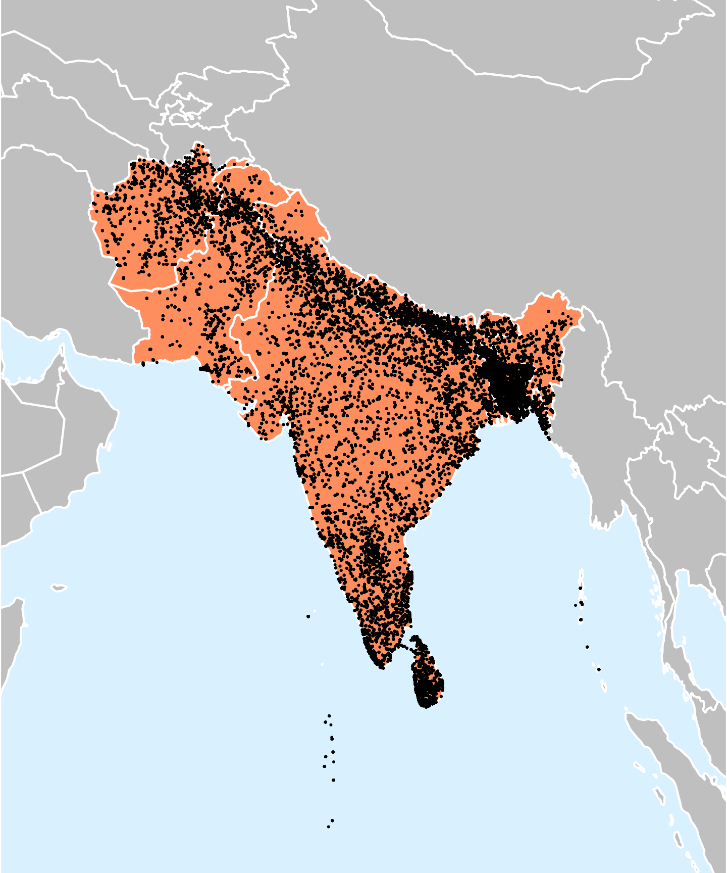
### All projects in some countries
```{r}
# projects <- qs2::qs_read("data/data-processed/recipients_projects.qs2")

# projects_s_asia <- projects |>
#   mutate(
#     region = countrycode(iso_a3, origin = "iso3c", destination = "region")
#   ) |>
#   filter(region == "South Asia") |>
#   st_drop_geometry() |>
#   unnest_wider(project_details) |>
#   unnest(projects_in_country) |>
#   select(iso_a3, name, project_id, geometry) |>
#   st_set_geometry("geometry")

# qs2::qs_save(projects_s_asia, "data/data-processed/projects_s_asia.qs2")
```
```{r}
#| fig-width: 5
#| fig-height: 6
projects_s_asia <- qs2::qs_read(here::here("data/data-processed/projects_s_asia.qs2"))

world_with_regions <- world |>
  mutate(is_south_asia = region_wb == "South Asia")

# Make a little bounding box with these specific coordinates to to zoom in
bbox <- st_bbox(
  c(xmin = 60, xmax = 100, ymin = -1, ymax = 45),
  crs = st_crs("EPSG:4326")
) |>
  st_as_sfc() |>
  st_transform("+proj=eqearth") |>
  st_bbox()

ggplot() +
  geom_sf(data = world_with_regions, aes(fill = is_south_asia), color = "white", linewidth = 0.5) +
  geom_sf(data = projects_s_asia, size = 0.05) +
  scale_fill_manual(values = c("grey75", clrs[3]), guide = "none") +
  coord_sf(
    crs = "+proj=eqearth",
    xlim = c(bbox["xmin"], bbox["xmax"]),
    ylim = c(bbox["ymin"], bbox["ymax"]),
    datum = NA
  ) +
  theme_void() +
  theme(panel.background = element_rect(fill = "#d9f0ff"))
```
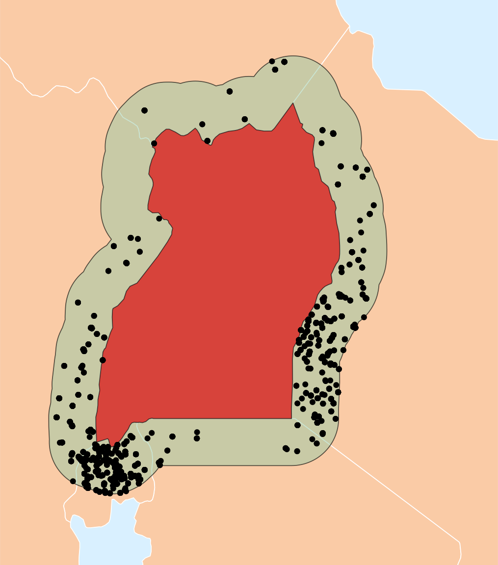
### Projects in border area
```{r}
# projects <- qs2::qs_read("data/data-processed/recipients_projects.qs2")

# uganda_projects <- projects |>
#   filter(iso_a3 == "UGA")

# qs2::qs_save(uganda_projects, "data/data-processed/uganda_projects.qs2")
```
```{r}
uganda <- world |> filter(admin == "Uganda")

# Find all neighboring countries
neighbors <- st_filter(world, uganda, .predicate = st_touches)
```
```{r}
uganda_projects <- qs2::qs_read(here::here("data/data-processed/uganda_projects.qs2"))

uganda_neighbor_projects <- uganda_projects |>
  st_drop_geometry() |>
  unnest_wider(project_details) |>
  unnest(projects_outside_border_long) |>
  st_set_geometry("geometry") |>
  filter(year == 2019)

uganda_buffer <- uganda_projects |>
  st_drop_geometry() |>
  unnest_wider(project_details) |>
  pull(border_buffer)
```
```{r}
#| fig-width: 3.525
#| fig-height: 4
# Make a little bounding box with these specific coordinates to to zoom in
bbox <- st_bbox(
  c(xmin = 28, xmax = 38, ymin = -3, ymax = 5.5),
  crs = st_crs("EPSG:4326")
) |>
  st_as_sfc() |>
  st_transform("+proj=eqearth") |>
  st_bbox()

ggplot() +
  geom_sf(data = neighbors, fill = "#facba6", color = "white") +
  geom_sf(data = uganda_buffer, fill = clrs[5], alpha = 0.5) +
  geom_sf(data = uganda, fill = clrs[1]) +
  geom_sf(data = uganda_neighbor_projects, size = 0.75) +
  coord_sf(
    crs = "+proj=eqearth",
    xlim = c(bbox["xmin"], bbox["xmax"]),
    ylim = c(bbox["ymin"], bbox["ymax"])
  ) +
  theme_void() +
  theme(panel.background = element_rect(fill = "#d9f0ff"))
```
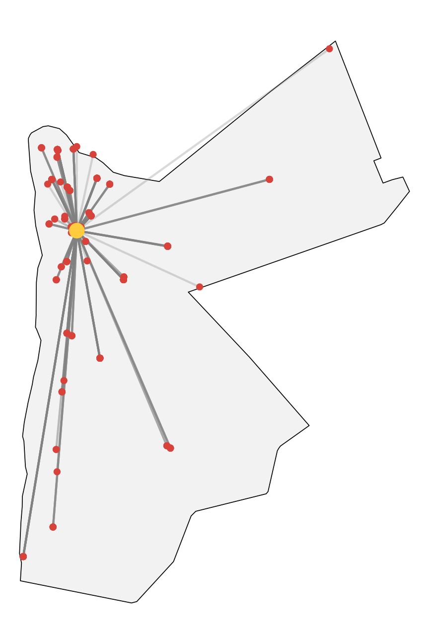
### Project distance from capital
```{r}
# projects <- qs2::qs_read("data/data-processed/recipients_projects.qs2")

# jordan_projects <- projects |>
#   filter(iso_a3 == "JOR")

# qs2::qs_save(jordan_projects, "data/data-processed/jordan_projects.qs2")
```
```{r}
#| fig-width: 3
#| fig-height: 4.5
jordan_projects <- qs2::qs_read(here::here(
  "data/data-processed/jordan_projects.qs2"
))

jordan_internal_projects <- jordan_projects |>
  st_drop_geometry() |>
  unnest_wider(project_details) |>
  unnest(projects_in_country_long) |>
  st_set_geometry("geometry") |>
  filter(year == 2019)

jordan <- world |> filter(iso_a3 == "JOR")

# Create LINESTRINGs between each project and the capital
jordan_with_lines <- jordan_internal_projects |>
  mutate(
    line_geom = map2(capital_geom, geometry, \(cap, proj) {
      st_linestring(rbind(
        st_coordinates(cap),
        st_coordinates(proj)
      ))
    })
  ) |>
  mutate(line_geom = st_sfc(line_geom, crs = st_crs(jordan))) |>
  st_set_geometry("line_geom")

# Extract Amman
jordan_capital <- jordan_internal_projects |>
  slice(1) |>
  select(capital_name, capital_geom) |>
  st_set_geometry("capital_geom")

ggplot() +
  geom_sf(data = jordan, fill = "grey95", color = "black") +
  geom_sf(data = jordan_with_lines, alpha = 0.3, color = "grey50") +
  geom_sf(data = jordan_internal_projects, color = clrs[1], size = 1) +
  geom_sf(data = jordan_capital, color = clrs[4], size = 3) +
  theme_void()
```
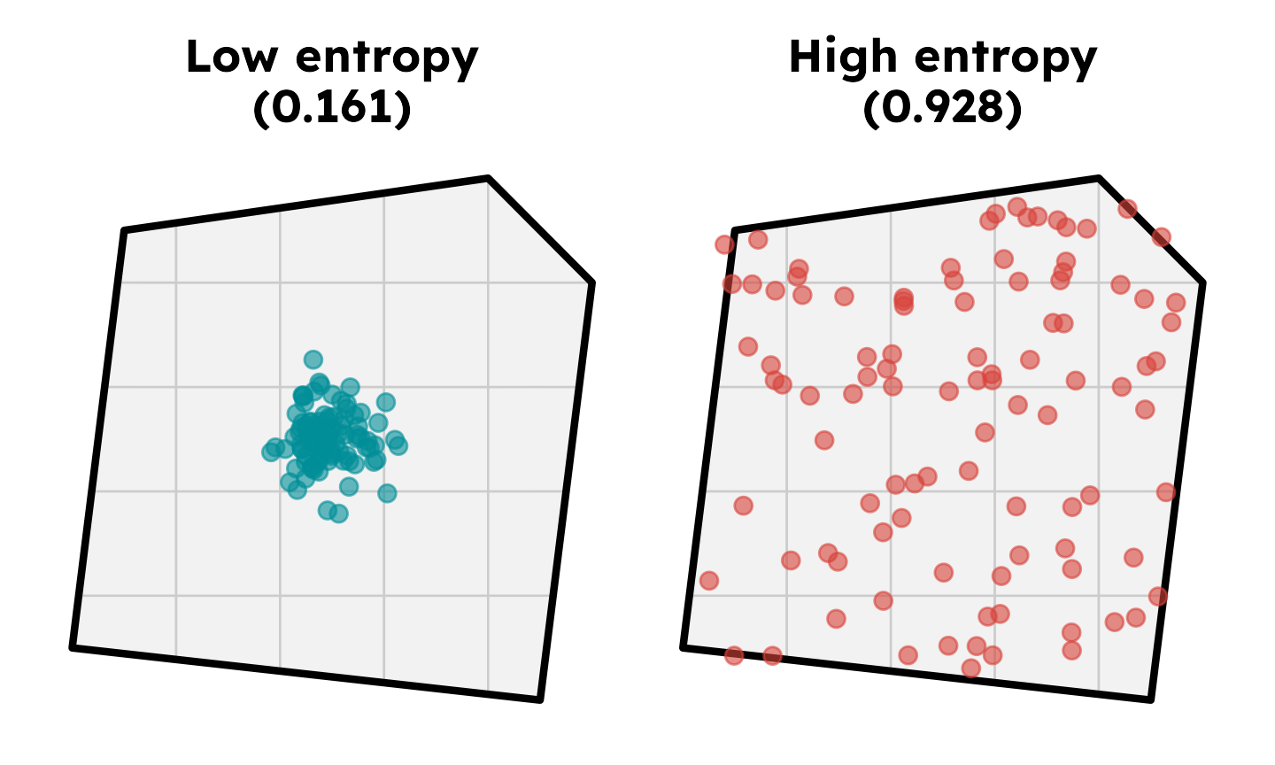
### Project entropy
```{r}
library(entropy)
calc_entropy_from_points <- function(projects, grid) {
  project_counts <- st_join(projects, grid) |>
    st_drop_geometry() |>
    count(grid_id) |>
    complete(grid_id = 1:nrow(grid), fill = list(n = 0))

  shannon <- entropy::entropy(project_counts$n, method = "ML")
  normalized <- shannon / log(nrow(grid))

  return(list(shannon = shannon, normalized = normalized))
}
```
```{r}
#| warning: false
#| message: false
# Make up a fake country
country <- st_polygon(list(
  matrix(c(
    0, 1,  # Bottom left
    9, 0,  # Bottom right
    10, 8, # Right side
    8, 10, # Top right
    1, 9,  # Top left
    0, 1   # Close the polygon
  ), ncol = 2, byrow = TRUE)
)) |>
  st_sfc(crs = 4326) |>
  st_sf()

# Make a grid that's cropped to the country
grid <- st_make_grid(country, n = c(5, 5), square = TRUE) |>
  st_sf() |>
  mutate(grid_id = row_number()) |>
  st_intersection(country) |>
  st_make_valid()

# Create some fake projects with different kinds of dispersement
n_projects <- 100

withr::with_seed(1234, {
  low_entropy_projects <- tibble(
    x = rnorm(n_projects, mean = 5, sd = 0.5),
    y = rnorm(n_projects, mean = 5, sd = 0.5)
  ) |>
    st_as_sf(coords = c("x", "y"), crs = 4326)

  high_entropy_projects <- tibble(
    x = runif(n_projects, min = 0.5, max = 9.5),
    y = runif(n_projects, min = 0.5, max = 9.5)
  ) |>
    st_as_sf(coords = c("x", "y"), crs = 4326)
})

entropy_low <- calc_entropy_from_points(low_entropy_projects, grid)
entropy_high <- calc_entropy_from_points(high_entropy_projects, grid)
```
```{r}
#| fig-width: 5
#| fig-height: 3
p_low <- ggplot() +
  geom_sf(data = grid, fill = "grey95", color = "grey80", linewidth = 0.3) +
  geom_sf(data = country, fill = NA, color = "black", linewidth = 1) +
  geom_sf(
    data = low_entropy_projects,
    color = clrs[6],
    alpha = 0.6,
    size = 2
  ) +
  labs(title = glue::glue("Low entropy\n({round(entropy_low$normalized, 3)})")) +
  theme_ngo() +
  theme(
    panel.grid = element_blank(),
    axis.text = element_blank(),
    plot.title = element_text(hjust = 0.5)
  )

p_high <- ggplot() +
  geom_sf(data = grid, fill = "grey95", color = "grey80", linewidth = 0.3) +
  geom_sf(data = country, fill = NA, color = "black", linewidth = 1) +
  geom_sf(
    data = high_entropy_projects,
    color = clrs[1],
    alpha = 0.6,
    size = 2
  ) +
  labs(title = glue::glue("High entropy\n({round(entropy_high$normalized, 3)})")) +
  theme_ngo() +
  theme(
    panel.grid = element_blank(),
    axis.text = element_blank(),
    plot.title = element_text(hjust = 0.5)
  )

(p_low | p_high)
```
## Outcome 1 = projects in neighbors
(TODO: different buffer sizes)
### Treatment: CCSI
Treatment models and weights:
```{r}
# Treatment given history + confounders
denom_model_ccsi <- lm(
ccsi ~ ccsi_lag + ccsi_lag2 + ccsi_cumsum_lag3 +
polyarchy_lag + corruption_lag + rule_law_lag +
civil_liberties_lag + physical_violence_lag +
factor(year),
data = panel_lags
)
# Treatment given history only
num_model_ccsi <- lm(
ccsi ~ ccsi_lag + ccsi_lag2 + ccsi_cumsum_lag3 + factor(year),
data = panel_lags
)
panel_lags_weights_ccsi <- panel_lags |>
mutate(
num_pred = predict(num_model_ccsi),
denom_pred = predict(denom_model_ccsi),
num_resid = ccsi - num_pred,
denom_resid = ccsi - denom_pred,
num_density = dnorm(ccsi, mean = num_pred, sd = sd(num_resid)),
denom_density = dnorm(ccsi, mean = denom_pred, sd = sd(denom_resid)),
iptw_ratio = num_density / denom_density
) |>
group_by(iso3) |>
mutate(iptw = cumprod(iptw_ratio)) |>
ungroup()
summary(panel_lags_weights_ccsi$iptw)
```
Outcome model:
```{r}
#| warning: false
#| message: false
#| fig-width: 6
#| fig-height: 4
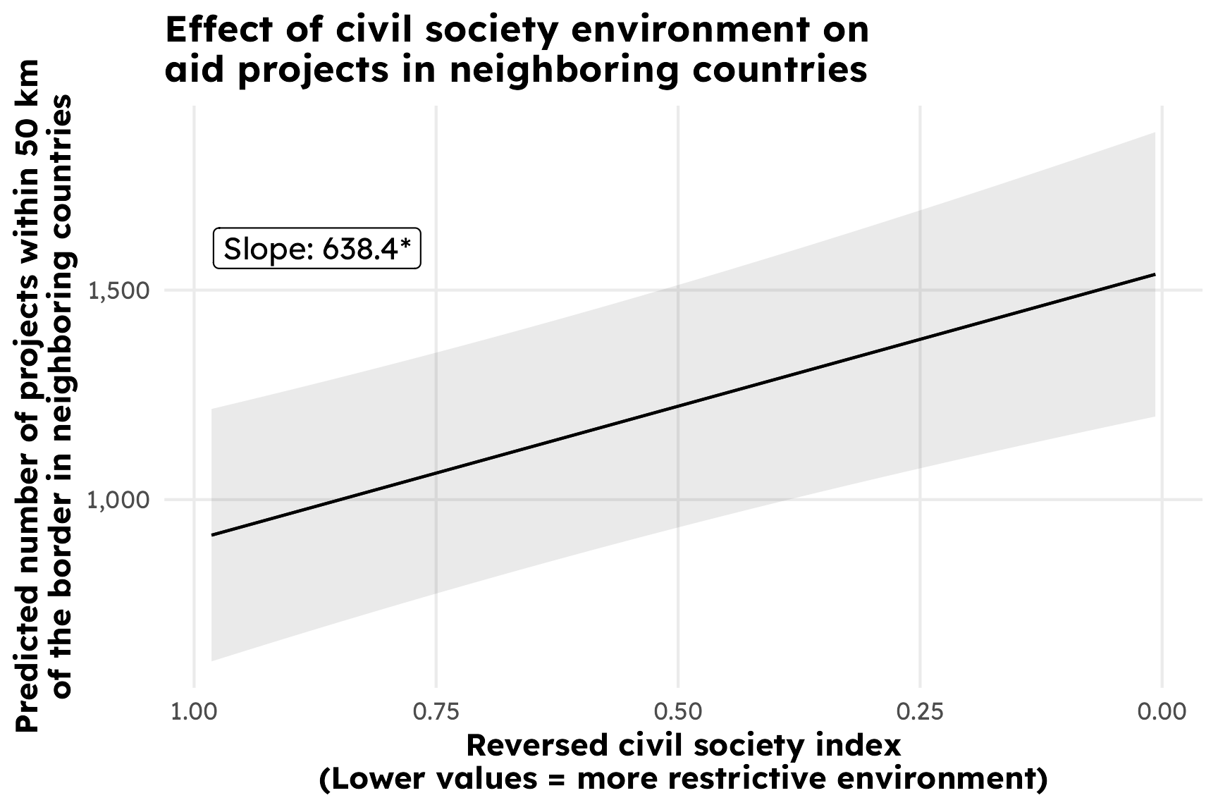
neighbor_model_msm <- lmer(
n_neighbor_projects ~ ccsi_lag + factor(year) + (1 | iso3),
data = panel_lags_weights_ccsi,
weights = iptw
)
neighbor_model_slope <- avg_slopes(neighbor_model_msm, variables = "ccsi_lag")
neighbor_model_slope
plot_predictions(neighbor_model_msm, condition = "ccsi_lag") +
annotate(
geom = "label",
x = 0.98,
y = 1600,
label = paste0(
"Slope: ",
round(-neighbor_model_slope$estimate, 1),
"*"
),
hjust = 0
) +
scale_x_reverse() +
scale_y_continuous(labels = label_comma()) +
labs(
x = "Reversed civil society index\n(Lower values = more restrictive environment)",
y = "Predicted number of projects within 50 km\nof the border in neighboring countries",
title = "Effect of civil society environment on\naid projects in neighboring countries"
) +
theme_ngo()
```
### Treatment: Laws
Treatment models and weights:
```{r}
# Treatment given history + confounders
denom_model_barriers <- lm(
barriers_total ~ barriers_total_lag + barriers_total_lag2 + barriers_total_cumsum_lag3 +
polyarchy_lag + corruption_lag + rule_law_lag +
civil_liberties_lag + physical_violence_lag +
factor(year),
data = panel_lags
)
# Treatment given history only
num_model_barriers <- lm(
barriers_total ~ barriers_total_lag + barriers_total_lag2 + barriers_total_cumsum_lag3 + factor(year),
data = panel_lags
)
# Get predicted values and residuals and stabilized weights
panel_lags_weights_barriers <- panel_lags |>
mutate(
num_pred = predict(num_model_barriers),
denom_pred = predict(denom_model_barriers),
num_resid = barriers_total - num_pred,
denom_resid = barriers_total - denom_pred,
num_density = dnorm(barriers_total, mean = num_pred, sd = sd(num_resid)),
denom_density = dnorm(barriers_total, mean = denom_pred, sd = sd(denom_resid)),
iptw_ratio = num_density / denom_density
) |>
group_by(iso3) |>
mutate(iptw = cumprod(iptw_ratio)) |>
ungroup()
summary(panel_lags_weights_barriers$iptw)
```
```{r}
# Treatment given history + confounders
denom_model_advocacy <- lm(
advocacy ~ advocacy_lag + advocacy_lag2 + advocacy_cumsum_lag3 +
polyarchy_lag + corruption_lag + rule_law_lag +
civil_liberties_lag + physical_violence_lag +
factor(year),
data = panel_lags
)
# Treatment given history only
num_model_advocacy <- lm(
advocacy ~ advocacy_lag + advocacy_lag2 + advocacy_cumsum_lag3 + factor(year),
data = panel_lags
)
# Get predicted values and residuals
panel_lags_weights_advocacy <- panel_lags |>
mutate(
num_pred = predict(num_model_advocacy),
denom_pred = predict(denom_model_advocacy),
num_resid = advocacy - num_pred,
denom_resid = advocacy - denom_pred
) |>
# Get stabilized weights
mutate(
num_density = dnorm(advocacy, mean = num_pred, sd = sd(num_resid)),
denom_density = dnorm(advocacy, mean = denom_pred, sd = sd(denom_resid)),
iptw_ratio = num_density / denom_density,
iptw = cumprod(iptw_ratio)
)
panel_lags_weights_advocacy <- panel_lags |>
mutate(
num_pred = predict(num_model_advocacy),
denom_pred = predict(denom_model_advocacy),
num_resid = advocacy - num_pred,
denom_resid = advocacy - denom_pred,
num_density = dnorm(advocacy, mean = num_pred, sd = sd(num_resid)),
denom_density = dnorm(advocacy, mean = denom_pred, sd = sd(denom_resid)),
iptw_ratio = num_density / denom_density
) |>
group_by(iso3) |>
mutate(iptw = cumprod(iptw_ratio)) |>
ungroup()
summary(panel_lags_weights_advocacy$iptw)
```
Outcome model:
```{r}
#| warning: false
#| message: false
#| fig-width: 6
#| fig-height: 4
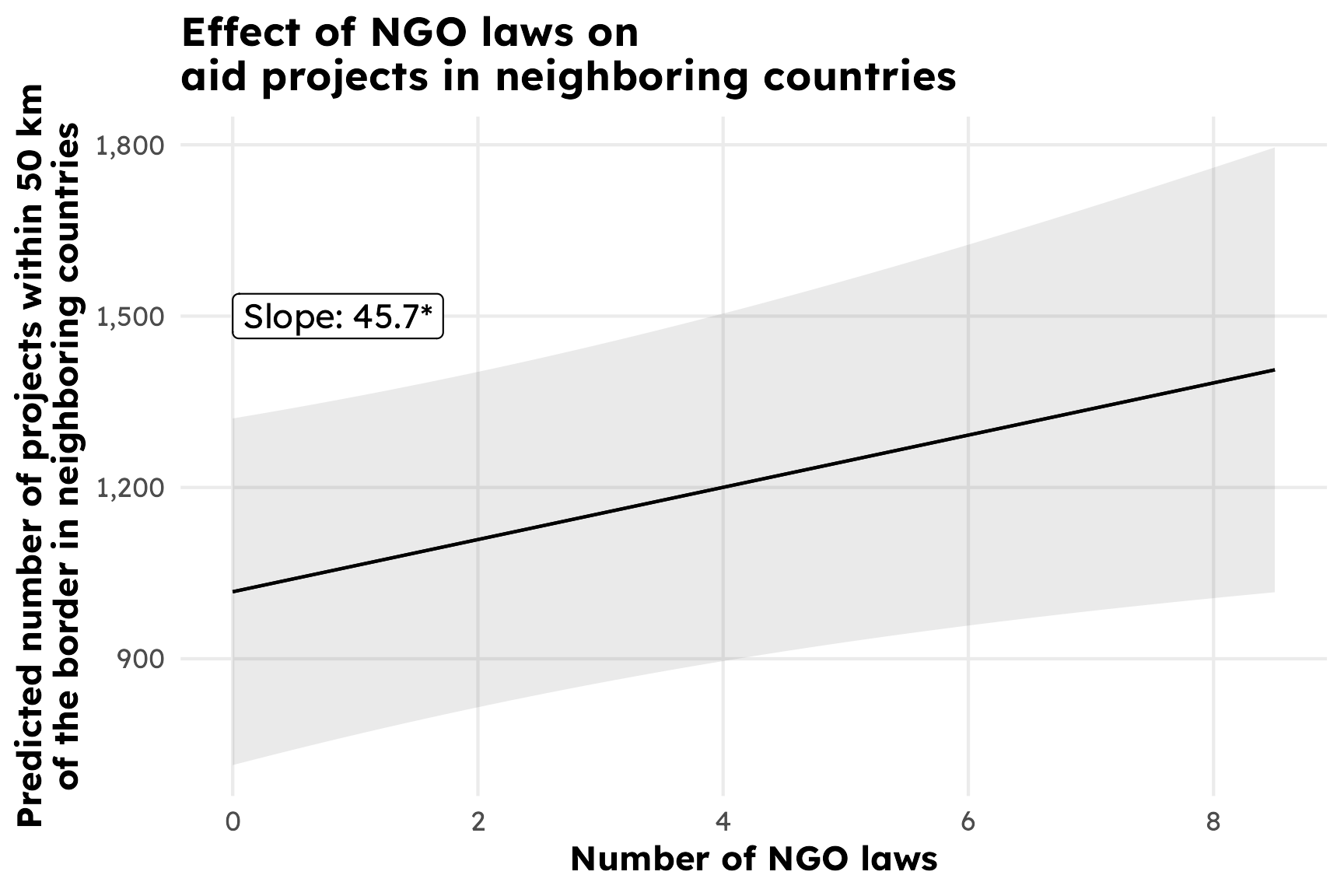
neighbor_model_msm_barriers <- lmer(
n_neighbor_projects ~ barriers_total_lag + factor(year) + (1 | iso3),
data = panel_lags_weights_barriers,
weights = iptw
)
neighbor_model_slope_barriers <- avg_slopes(neighbor_model_msm_barriers, variables = "barriers_total_lag")
neighbor_model_slope_barriers
plot_predictions(neighbor_model_msm_barriers, condition = "barriers_total_lag") +
annotate(
geom = "label",
x = 0,
y = 1500,
label = paste0(
"Slope: ",
round(neighbor_model_slope_barriers$estimate, 1),
"*"
),
hjust = 0
) +
scale_y_continuous(labels = label_comma()) +
labs(
x = "Number of NGO laws",
y = "Predicted number of projects within 50 km\nof the border in neighboring countries",
title = "Effect of NGO laws on\naid projects in neighboring countries"
) +
theme_ngo()
```
```{r}
#| warning: false
#| message: false
#| fig-width: 6
#| fig-height: 4
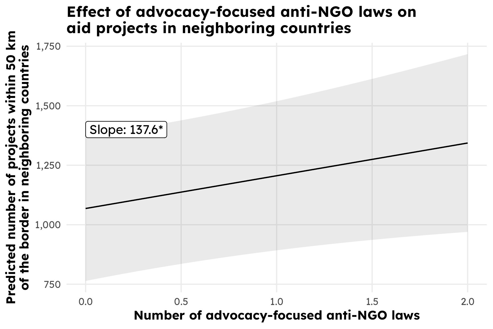
neighbor_model_msm_advocacy <- lmer(
n_neighbor_projects ~ advocacy_lag + factor(year) + (1 | iso3),
data = panel_lags_weights_advocacy,
weights = iptw
)
neighbor_model_slope_advocacy <- avg_slopes(neighbor_model_msm_advocacy, variables = "advocacy_lag")
neighbor_model_slope_advocacy
plot_predictions(neighbor_model_msm_advocacy, condition = "advocacy_lag") +
annotate(
geom = "label",
x = 0,
y = 1400,
label = paste0(
"Slope: ",
round(neighbor_model_slope_advocacy$estimate, 1),
"*"
),
hjust = 0
) +
scale_y_continuous(labels = label_comma()) +
labs(
x = "Number of advocacy-focused anti-NGO laws",
y = "Predicted number of projects within 50 km\nof the border in neighboring countries",
title = "Effect of advocacy-focused anti-NGO laws on\naid projects in neighboring countries"
) +
theme_ngo()
```
## Outcome 2 = projects within country
### Treatment: CCSI
#### Outcome 1: Distance from capital
```{r}
#| warning: false
#| message: false
#| fig-width: 6
#| fig-height: 4
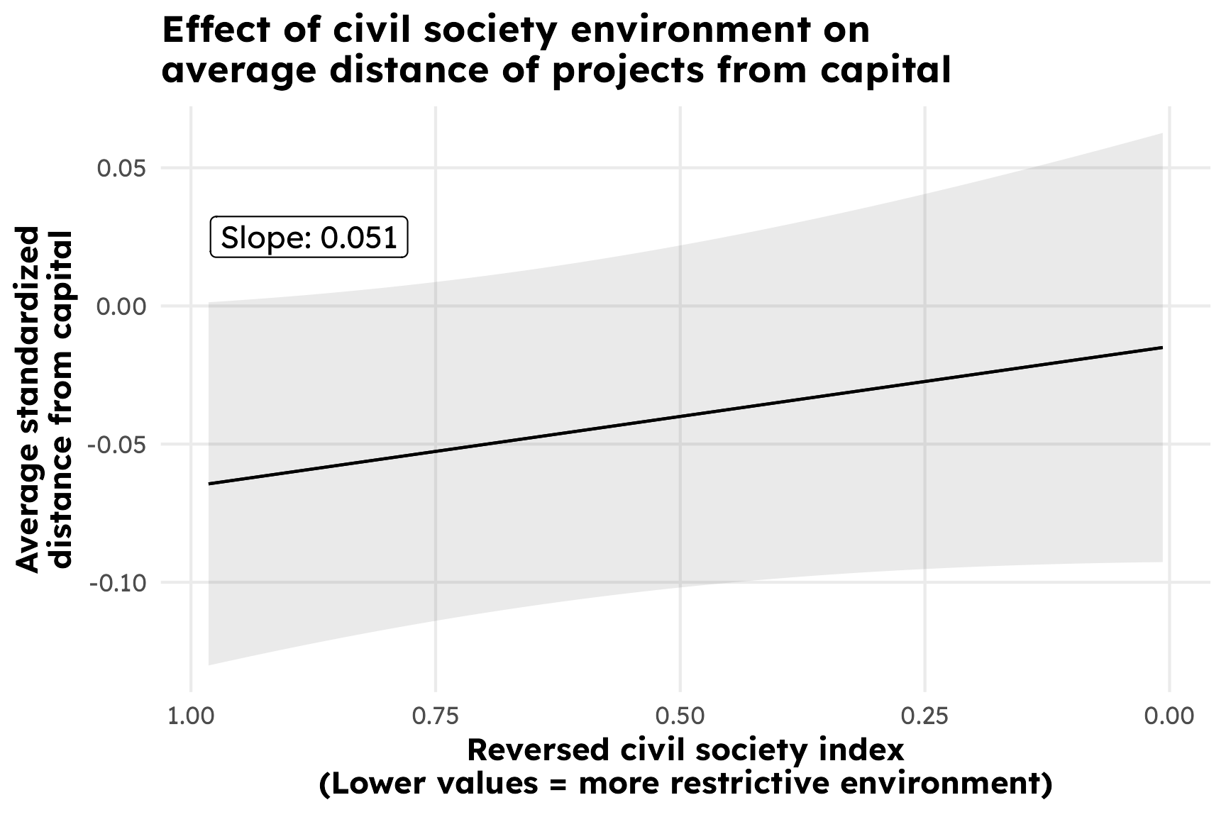
distance_model_msm <- lmer(
mean_dist_z ~ ccsi_lag + factor(year) + (1 | iso3),
data = panel_lags_weights_ccsi,
weights = iptw
)
distance_model_slope <- avg_slopes(distance_model_msm, variables = "ccsi_lag")
distance_model_slope
plot_predictions(distance_model_msm, condition = "ccsi_lag") +
annotate(
geom = "label",
x = 0.98,
y = 0.025,
label = paste0(
"Slope: ",
round(-distance_model_slope$estimate, 3)
),
hjust = 0
) +
scale_x_reverse() +
labs(
x = "Reversed civil society index\n(Lower values = more restrictive environment)",
y = "Average standardized\ndistance from capital",
title = "Effect of civil society environment on\naverage distance of projects from capital"
) +
theme_ngo()
```
#### Outcome 2: Entropy
```{r}
#| warning: false
#| message: false
#| fig-width: 6
#| fig-height: 4
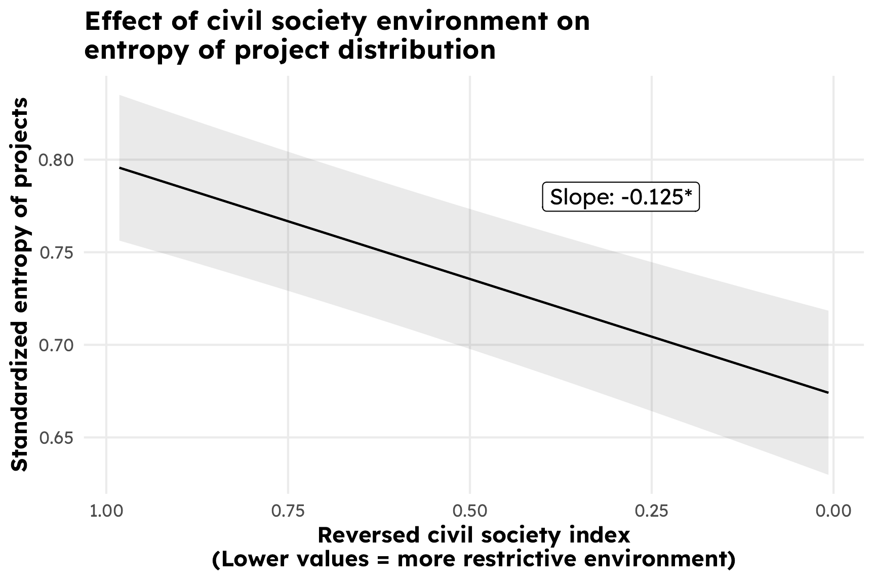
entropy_model_msm <- lmer(
normalized_entropy ~ ccsi_lag + factor(year) + (1 | iso3),
data = panel_lags_weights_ccsi,
weights = iptw
)
entropy_model_slope <- avg_slopes(entropy_model_msm, variables = "ccsi_lag")
entropy_model_slope
plot_predictions(entropy_model_msm, condition = "ccsi_lag") +
annotate(
geom = "label",
x = 0.4,
y = 0.78,
label = paste0(
"Slope: ",
round(-entropy_model_slope$estimate, 3),
"*"
),
hjust = 0
) +
scale_x_reverse() +
labs(
x = "Reversed civil society index\n(Lower values = more restrictive environment)",
y = "Standardized entropy of projects",
title = "Effect of civil society environment on\nentropy of project distribution"
) +
theme_ngo()
```
### Treatment: Laws
#### Outcome 1: Distance from capital
```{r}
#| warning: false
#| message: false
#| fig-width: 6
#| fig-height: 4
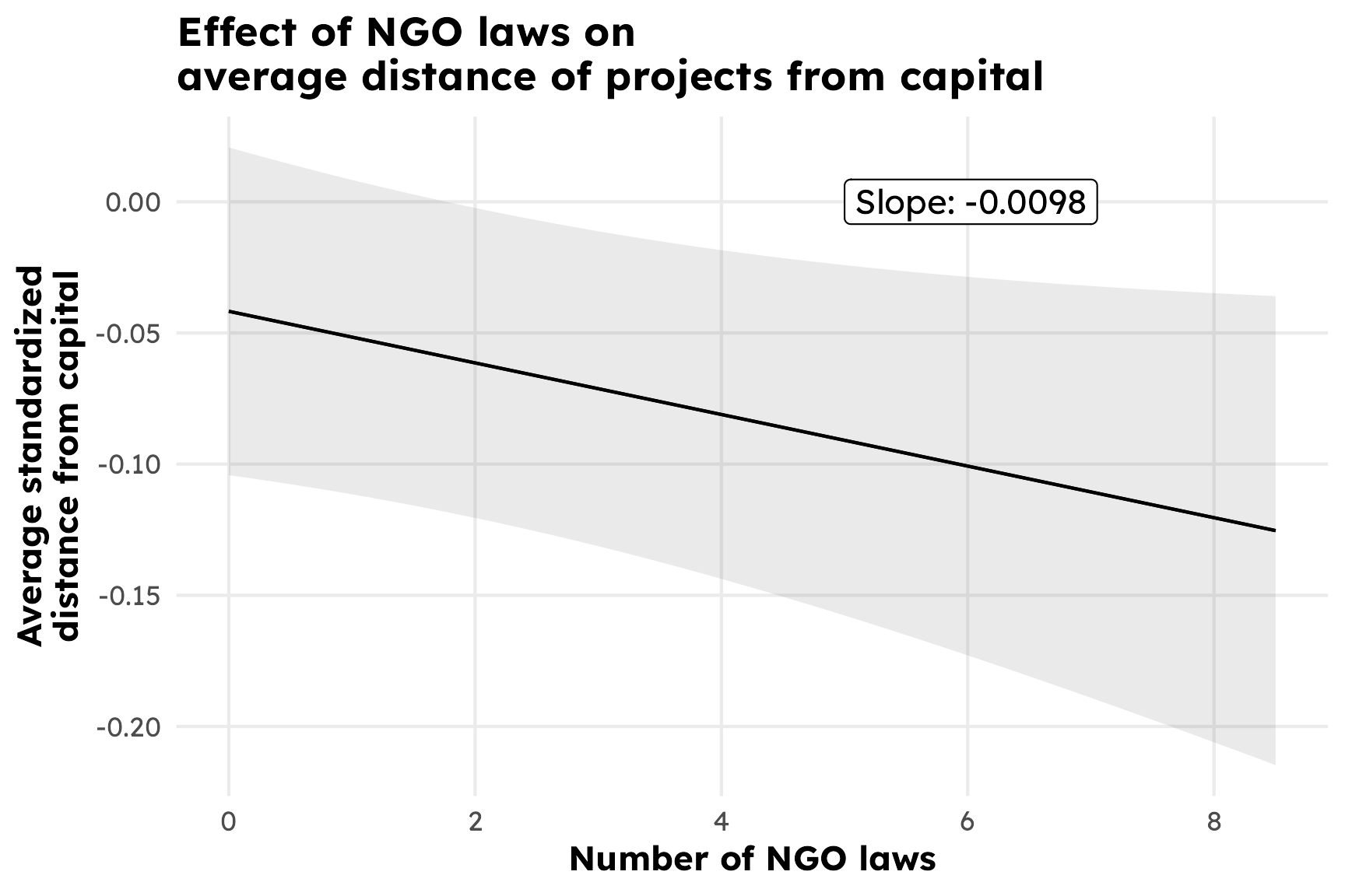
distance_model_msm_barriers <- lmer(
mean_dist_z ~ barriers_total_lag + factor(year) + (1 | iso3),
data = panel_lags_weights_barriers,
weights = iptw
)
distance_model_slope_barriers <- avg_slopes(distance_model_msm_barriers, variables = "barriers_total_lag")
distance_model_slope_barriers
plot_predictions(distance_model_msm_barriers, condition = "barriers_total_lag") +
annotate(
geom = "label",
x = 5,
y = 0,
label = paste0(
"Slope: ",
round(distance_model_slope_barriers$estimate, 4)
),
hjust = 0
) +
labs(
x = "Number of NGO laws",
y = "Average standardized\ndistance from capital",
title = "Effect of NGO laws on\naverage distance of projects from capital"
) +
theme_ngo()
```
```{r}
#| warning: false
#| message: false
#| fig-width: 6
#| fig-height: 4
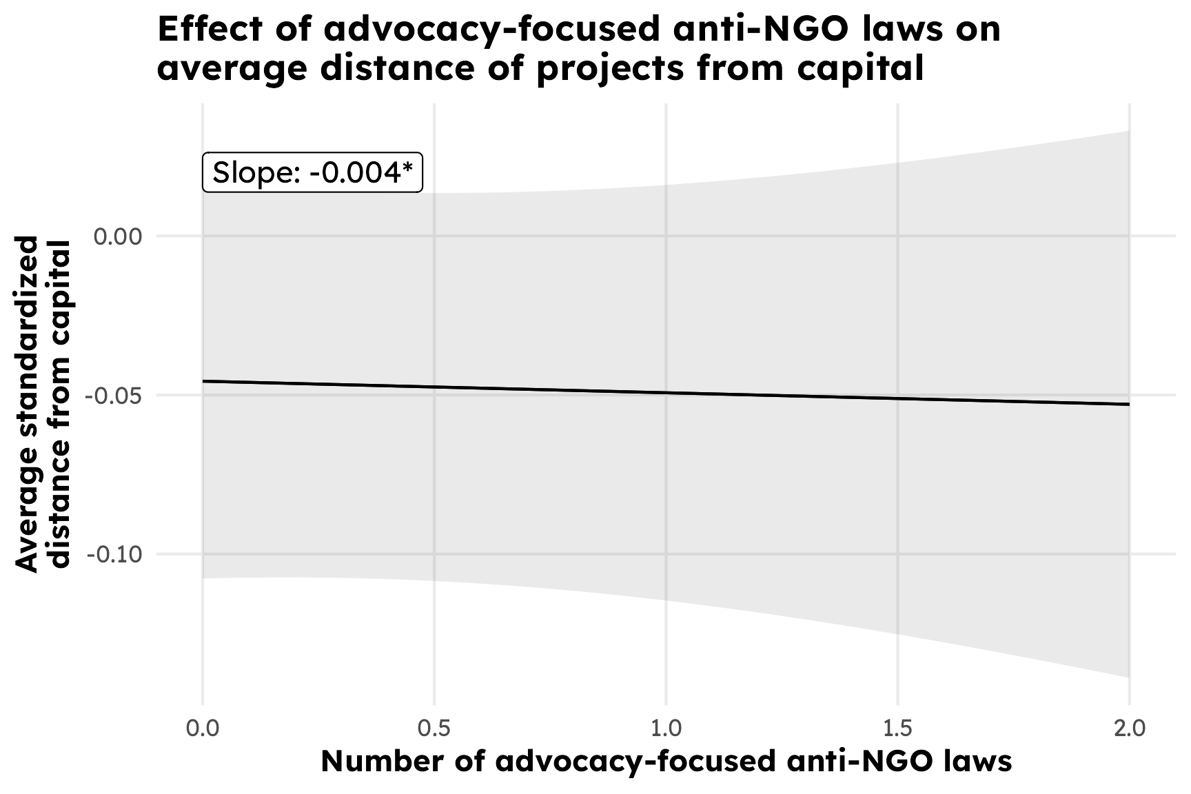
distance_model_msm_advocacy <- lmer(
mean_dist_z ~ advocacy_lag + factor(year) + (1 | iso3),
data = panel_lags_weights_advocacy,
weights = iptw
)
distance_model_slope_advocacy <- avg_slopes(distance_model_msm_advocacy, variables = "advocacy_lag")
distance_model_slope_advocacy
plot_predictions(distance_model_msm_advocacy, condition = "advocacy_lag") +
annotate(
geom = "label",
x = 0,
y = 0.02,
label = paste0(
"Slope: ",
round(distance_model_slope_advocacy$estimate, 3),
"*"
),
hjust = 0
) +
labs(
x = "Number of advocacy-focused anti-NGO laws",
y = "Average standardized\ndistance from capital",
title = "Effect of advocacy-focused anti-NGO laws on\naverage distance of projects from capital"
) +
theme_ngo()
```
#### Outcome 2: Entropy
```{r}
#| warning: false
#| message: false
#| fig-width: 6
#| fig-height: 4
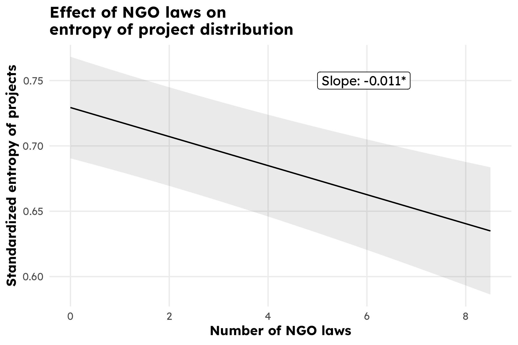
entropy_model_msm_barriers <- lmer(
normalized_entropy ~ barriers_total_lag + factor(year) + (1 | iso3),
data = panel_lags_weights_barriers,
weights = iptw
)
entropy_model_slope_barriers <- avg_slopes(entropy_model_msm_barriers, variables = "barriers_total_lag")
entropy_model_slope_barriers
plot_predictions(entropy_model_msm_barriers, condition = "barriers_total_lag") +
annotate(
geom = "label",
x = 5,
y = 0.75,
label = paste0(
"Slope: ",
round(entropy_model_slope_barriers$estimate, 3),
"*"
),
hjust = 0
) +
labs(
x = "Number of NGO laws",
y = "Standardized entropy of projects",
title = "Effect of NGO laws on\nentropy of project distribution"
) +
theme_ngo()
```
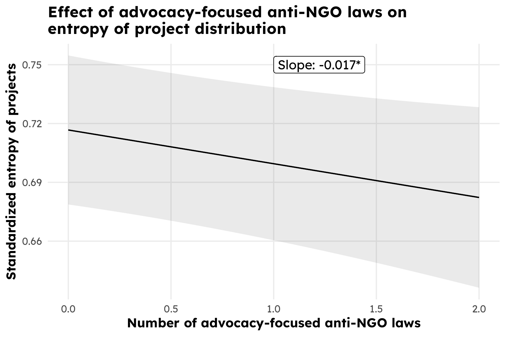
```{r}
#| warning: false
#| message: false
#| fig-width: 6
#| fig-height: 4
entropy_model_msm_advocacy <- lmer(
normalized_entropy ~ advocacy_lag + factor(year) + (1 | iso3),
data = panel_lags_weights_advocacy,
weights = iptw
)
entropy_model_slope_advocacy <- avg_slopes(entropy_model_msm_advocacy, variables = "advocacy_lag")
entropy_model_slope_advocacy
plot_predictions(entropy_model_msm_advocacy, condition = "advocacy_lag") +
annotate(
geom = "label",
x = 1,
y = 0.75,
label = paste0(
"Slope: ",
round(entropy_model_slope_advocacy$estimate, 3),
"*"
),
hjust = 0
) +
labs(
x = "Number of advocacy-focused anti-NGO laws",
y = "Standardized entropy of projects",
title = "Effect of advocacy-focused anti-NGO laws on\nentropy of project distribution"
) +
theme_ngo()
```