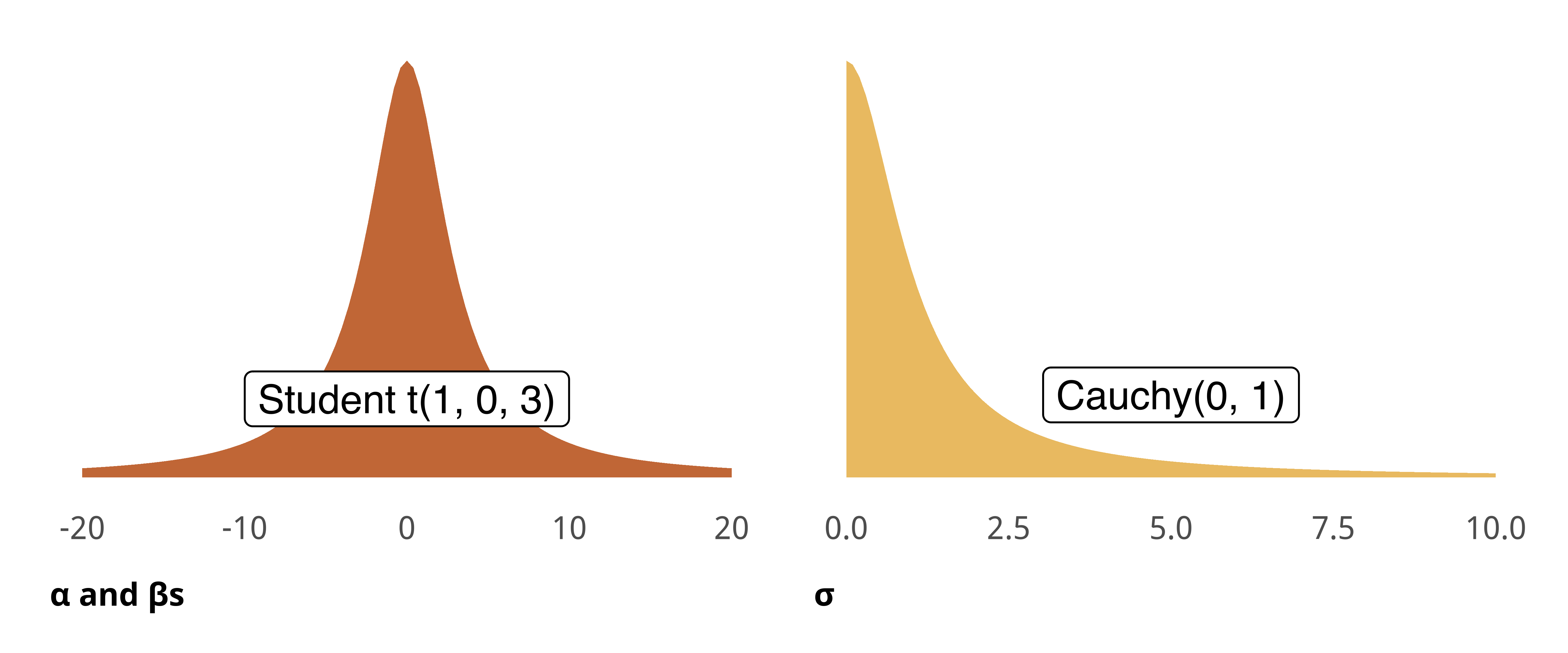
p1 <-ggplot() +stat_function(geom ="area", fun =~extraDistr::dlst(., df =1, mu =0, sigma =3), fill = clrs[2]) +xlim(c(-20, 20)) +annotate(geom ="label", x =0, y =0.02, label ="Student t(1, 0, 3)") +labs(x ="α and βs") +theme_pandem(prior =TRUE)p2 <-ggplot() +stat_function(geom ="area", fun =~dcauchy(., 0, 1), fill = clrs[4]) +xlim(c(0, 10)) +annotate(geom ="label", x =5, y =0.063, label ="Cauchy(0, 1)") +labs(x ="σ") +theme_pandem(prior =TRUE)p1 | p2
Prior simulation
Code
logit_priors <-c(prior(student_t(1, 0, 3), class = Intercept),prior(student_t(1, 0, 3), class = b),prior(cauchy(0, 1), class = sd, lb =0))model_policies_prior_only <-brm(bf(c7_internal_movement_bin ~ derogation_ineffect + new_cases_z + cumulative_cases_z + new_deaths_z + cumulative_deaths_z + prior_iccpr_derogations + prior_iccpr_other_action + v2x_rule + v2x_civlib + v2xcs_ccsi + year_week_num + (1| country_name)), data =filter(weekly_panel, c7_internal_movement_never ==0),family ="bernoulli",prior = logit_priors,sample_prior ="only",chains =4, seed = BAYES_SEED, iter =5000, refresh =0,threads =threading(2) # Two CPUs per chain to speed things up)## Start sampling## Running MCMC with 4 parallel chains, with 2 thread(s) per chain...## ## Chain 3 finished in 2.3 seconds.## Chain 2 finished in 2.7 seconds.## Chain 4 finished in 3.3 seconds.## Chain 1 finished in 4.2 seconds.## ## All 4 chains finished successfully.## Mean chain execution time: 3.1 seconds.## Total execution time: 4.4 seconds.model_policies_prior_only## Family: bernoulli ## Links: mu = logit ## Formula: c7_internal_movement_bin ~ derogation_ineffect + new_cases_z + cumulative_cases_z + new_deaths_z + cumulative_deaths_z + prior_iccpr_derogations + prior_iccpr_other_action + v2x_rule + v2x_civlib + v2xcs_ccsi + year_week_num + (1 | country_name) ## Data: filter(weekly_panel, c7_internal_movement_never == (Number of observations: 9246) ## Draws: 4 chains, each with iter = 5000; warmup = 2500; thin = 1;## total post-warmup draws = 10000## ## Group-Level Effects: ## ~country_name (Number of levels: 134) ## Estimate Est.Error l-95% CI u-95% CI Rhat Bulk_ESS Tail_ESS## sd(Intercept) 6.00 58.19 0.04 28.53 1.00 13079 5192## ## Population-Level Effects: ## Estimate Est.Error l-95% CI u-95% CI Rhat Bulk_ESS Tail_ESS## Intercept -108.55 1493.96 -1711.98 1031.23 1.01 1999 738## derogation_ineffect 2.25 49.17 -34.81 34.66 1.00 1783 660## new_cases_z -0.20 30.49 -32.87 37.03 1.01 5681 1582## cumulative_cases_z 7.21 85.03 -33.25 43.15 1.01 1563 592## new_deaths_z -2.44 32.18 -40.71 26.63 1.00 4081 1211## cumulative_deaths_z -0.00 24.71 -36.11 35.24 1.00 1944 992## prior_iccpr_derogationsTRUE 1.23 25.17 -28.96 39.09 1.00 1645 731## prior_iccpr_other_actionTRUE -6.56 52.41 -81.13 33.02 1.01 407 120## v2x_rule -0.25 13.93 -25.09 25.63 1.00 7747 2177## v2x_civlib 0.22 21.33 -29.93 30.17 1.00 4509 1462## v2xcs_ccsi 0.55 27.02 -29.45 32.71 1.01 2549 714## year_week_num 3.16 42.66 -29.48 49.76 1.01 2458 745## ## Draws were sampled using sample(hmc). For each parameter, Bulk_ESS## and Tail_ESS are effective sample size measures, and Rhat is the potential## scale reduction factor on split chains (at convergence, Rhat = 1).
Code
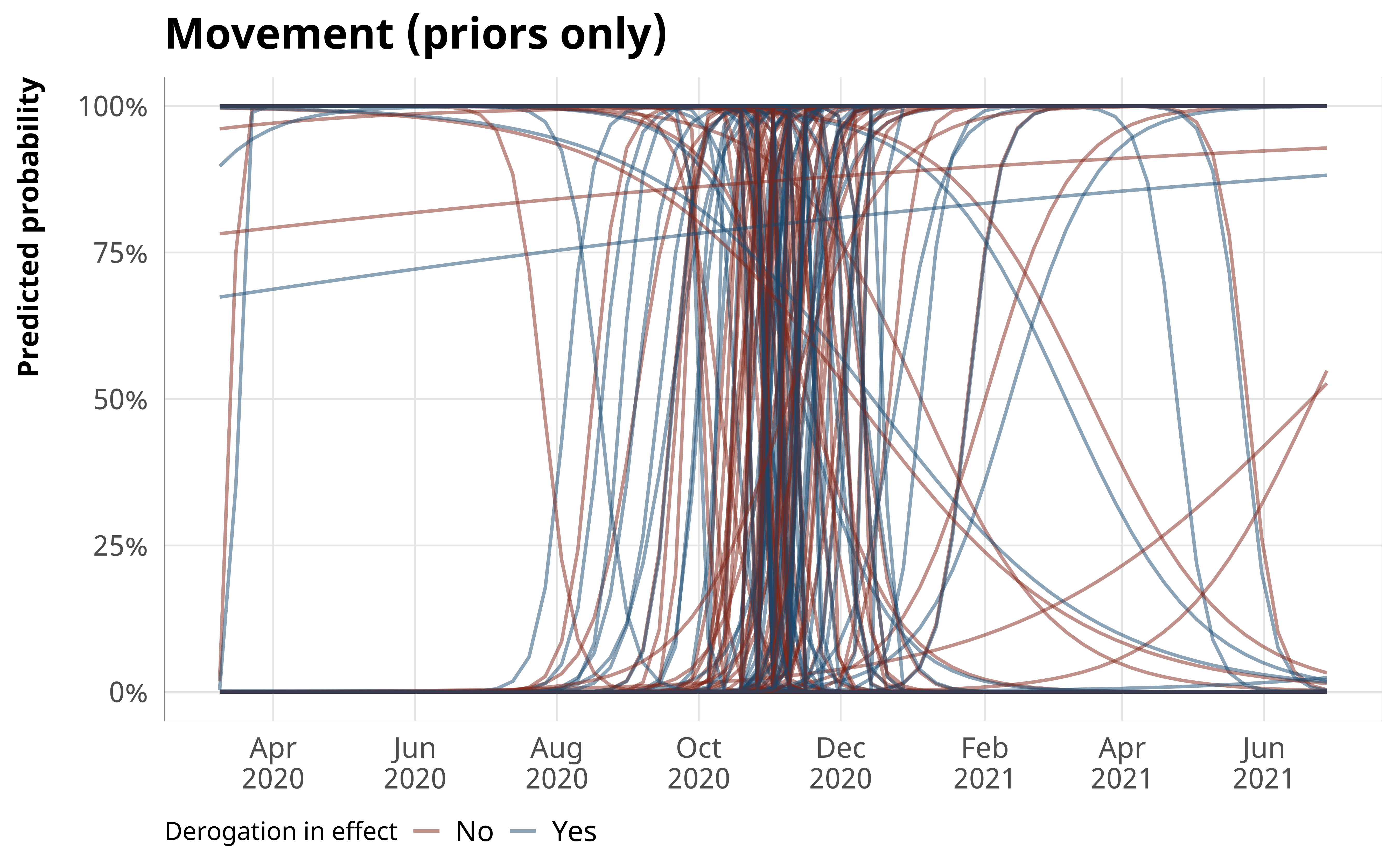
datagrid(model = model_policies_prior_only,year_week_num =1:69,derogation_ineffect =0:1) %>%add_epred_draws(model_policies_prior_only, ndraws =100) %>%left_join(year_week_lookup, by ="year_week_num") %>%mutate(derogation_ineffect =factor(derogation_ineffect, levels =0:1,labels =c("No", "Yes"),ordered =TRUE)) %>%ggplot(aes(x = year_week_day, y = .epred, color = derogation_ineffect)) +geom_line(aes(group =paste(.draw, derogation_ineffect)), alpha =0.5, linewidth =0.5) +scale_color_manual(values =c(clrs[1], clrs[8])) +scale_x_date(date_breaks ="2 months", date_labels ="%b\n%Y") +scale_y_continuous(labels =label_percent()) +labs(x =NULL, y ="Predicted probability", color ="Derogation in effect",title ="Movement (priors only)") +theme_pandem()
Posterior
Code
notes <-c("Estimates are median posterior log odds from ordered logistic and binary logistic regression models; 95% credible intervals (highest density posterior interval, or HDPI) in brackets.", "Total \\(R^2\\) considers the variance of both population and group effects;", "marginal \\(R^2\\) only takes population effects into account.")modelsummary(models_tbl_policies,estimate ="{estimate}",statistic ="[{conf.low}, {conf.high}]",coef_map = coef_map,gof_map = gof_map,output ="kableExtra",fmt =list(estimate =2, conf.low =2, conf.high =2)) %>%kable_styling(htmltable_class ="table-sm light-border") %>%footnote(general = notes, footnote_as_chunk =TRUE)
Cancel Public Events
Gathering Restrictions
Close Public Transit
Movement
International Travel
Derogation in effect
3.40
10.66
1.04
1.69
7.48
[1.39, 6.09]
[2.28, 42.56]
[0.64, 1.46]
[1.23, 2.18]
[0.31, 63.21]
New cases (standardized)
2.24
8.50
−0.67
0.76
6.50
[−0.62, 5.74]
[5.75, 11.66]
[−0.87, −0.48]
[0.28, 1.24]
[−0.22, 16.85]
Cumulative cases (standardized)
3.40
4.70
−0.36
−0.19
1.40
[1.32, 5.69]
[2.99, 6.88]
[−0.84, 0.03]
[−0.57, 0.21]
[−5.72, 14.59]
New deaths (standardized)
8.10
2.42
1.24
0.75
−1.62
[5.04, 11.58]
[1.07, 3.89]
[0.97, 1.53]
[0.38, 1.14]
[−3.26, −0.24]
Cumulative deaths (standardized)
−0.92
−2.70
0.71
0.19
6.01
[−1.90, 0.01]
[−3.64, −1.89]
[0.27, 1.15]
[−0.20, 0.63]
[0.80, 12.26]
Past ICCPR derogation
0.40
−1.24
0.07
0.15
−1.21
[−0.87, 1.60]
[−2.30, −0.15]
[−0.68, 0.83]
[−0.67, 0.95]
[−3.71, 0.84]
Past ICCPR action
−0.13
0.18
−0.26
0.05
0.33
[−1.26, 1.10]
[−0.90, 1.14]
[−0.99, 0.54]
[−0.67, 0.88]
[−1.76, 2.42]
Rule of law
3.28
0.79
−0.76
−0.72
−0.09
[1.10, 5.53]
[−1.00, 2.52]
[−2.25, 0.50]
[−2.12, 0.64]
[−4.05, 3.59]
Civil liberties
−4.18
1.18
1.06
−0.63
0.94
[−8.13, −0.64]
[−1.79, 4.01]
[−1.03, 3.58]
[−2.98, 1.58]
[−3.92, 7.87]
Core civil society index
0.34
0.01
−0.88
−0.64
−1.82
[−1.93, 2.94]
[−2.00, 2.08]
[−2.52, 0.71]
[−2.34, 0.95]
[−7.18, 2.25]
Constant
8.09
4.80
1.31
3.55
10.92
[6.64, 9.53]
[3.61, 6.00]
[0.55, 2.19]
[2.70, 4.45]
[6.96, 15.16]
Year-week
−0.02
−0.003
−0.01
−0.03
0.05
[−0.03, −0.02]
[−0.008, 0.002]
[−0.01, −0.007]
[−0.04, −0.03]
[0.03, 0.07]
Country random effects σ
2.45
2.32
1.79
1.92
3.90
[1.99, 2.95]
[1.96, 2.74]
[1.56, 2.05]
[1.66, 2.21]
[2.51, 5.51]
N
9453
9522
8832
9246
9591
\(R^2\) (total)
0.31
0.41
0.36
0.40
0.32
\(R^2\) (marginal)
0.01
0.03
0.07
0.12
0.0002
Note: Estimates are median posterior log odds from ordered logistic and binary logistic regression models; 95% credible intervals (highest density posterior interval, or HDPI) in brackets. Total \(R^2\) considers the variance of both population and group effects; marginal \(R^2\) only takes population effects into account.