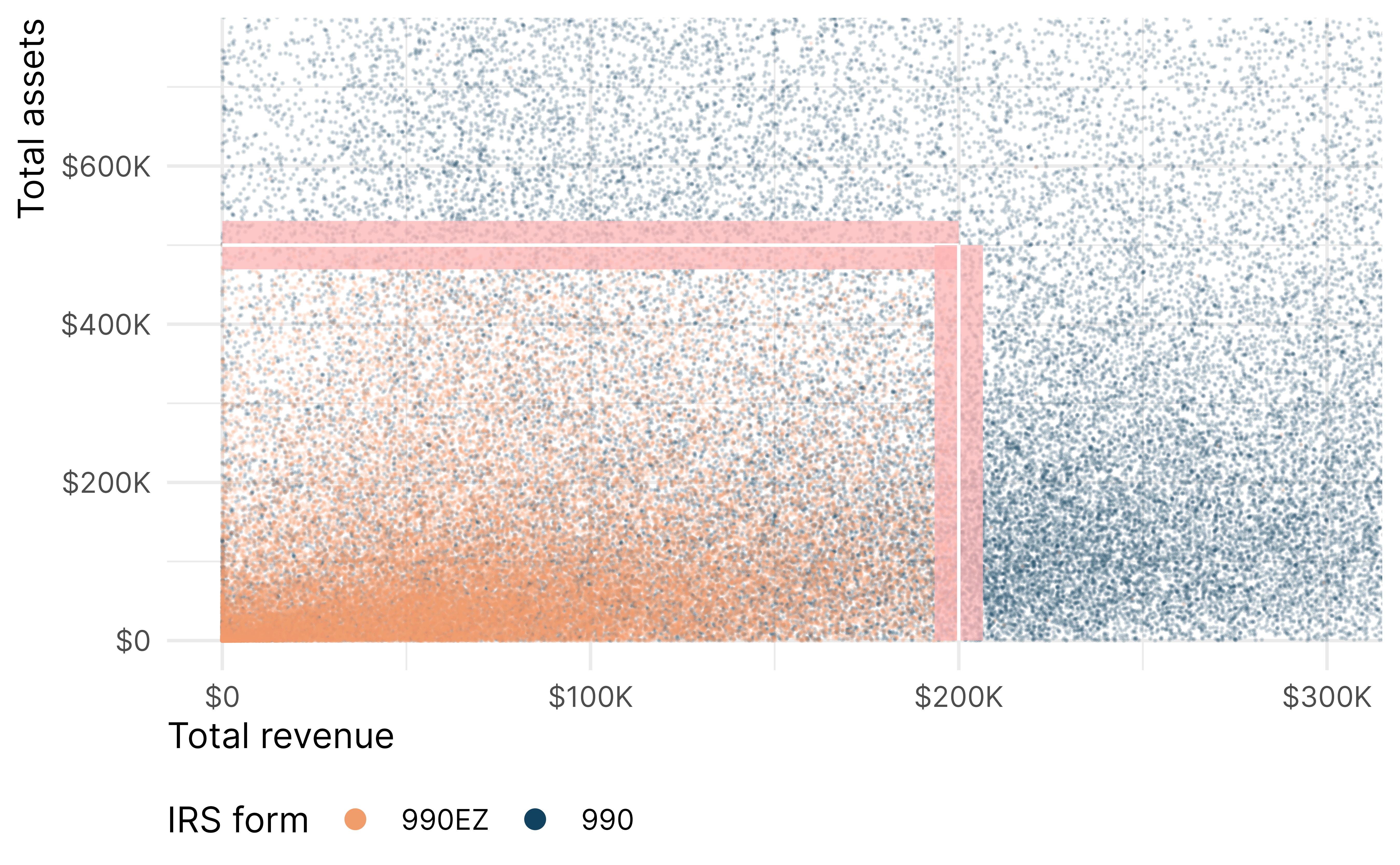
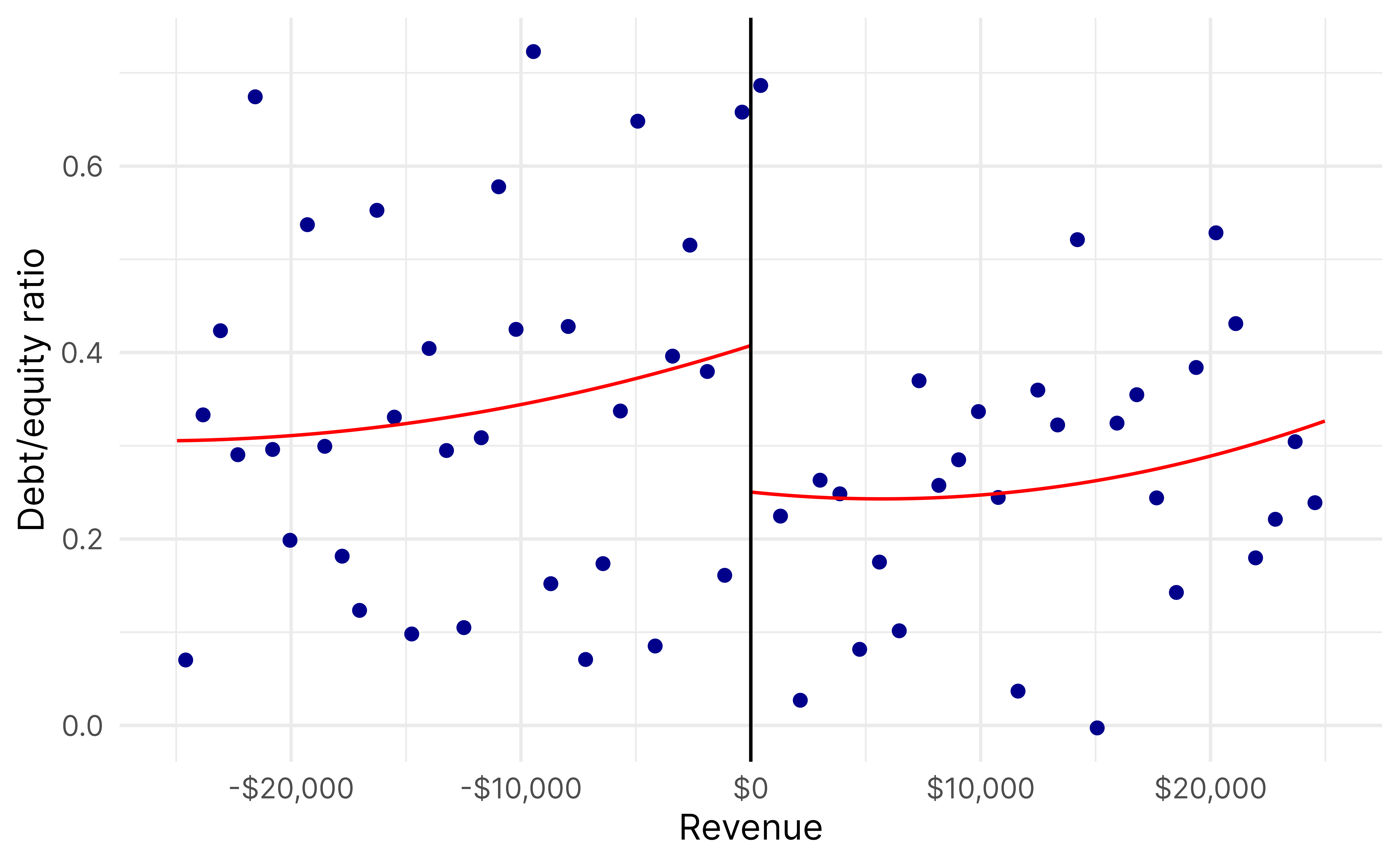
For causal inference purposes, we look at comparable nonprofts within a narrow bandwidth around the cutoff, but we have to look at both cutoffs simultaneously, creating this L-shape—organizations below and to the left of the two boundaries are treated, while organizations above and to the right are untreated.
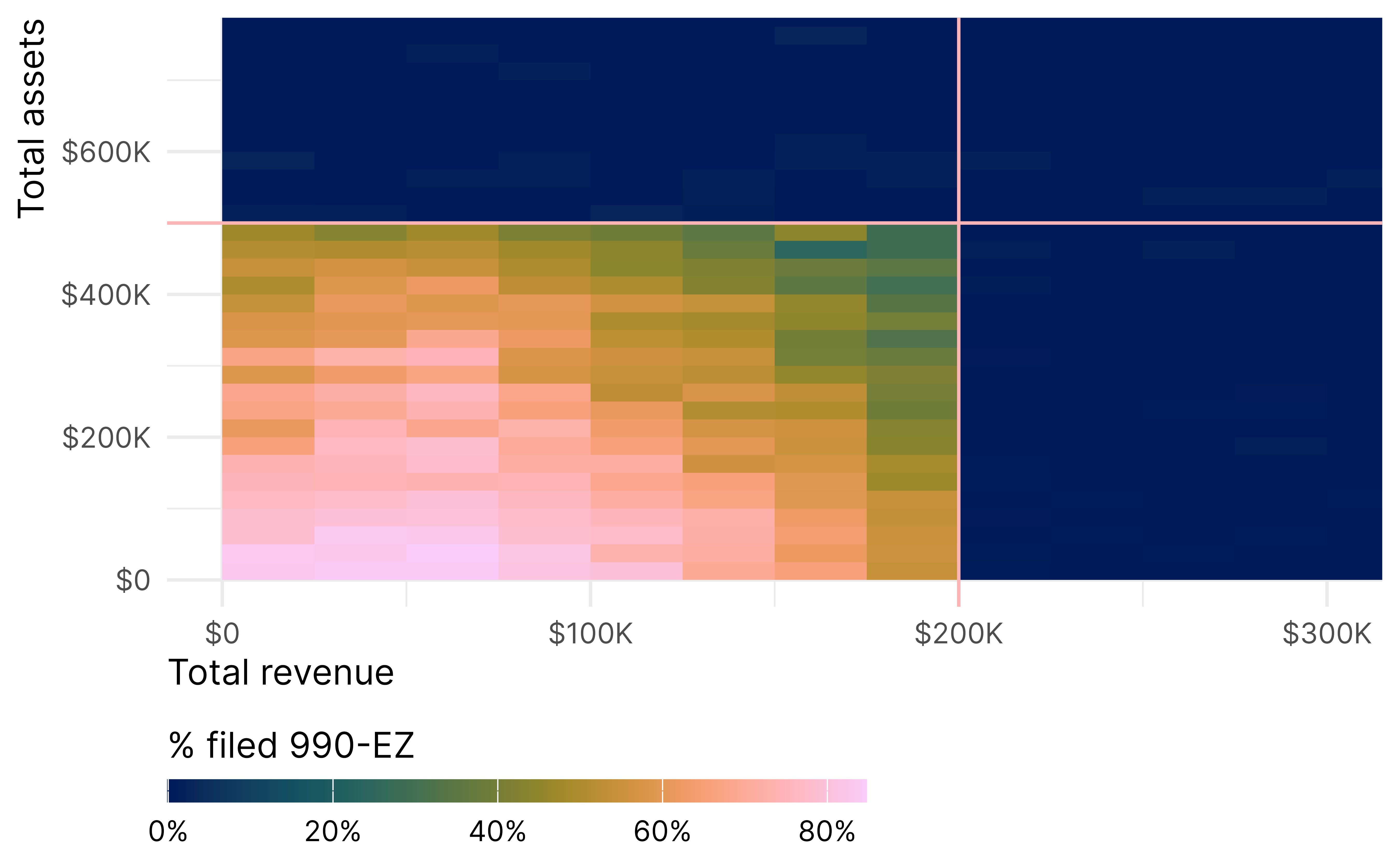
Further complicating things, there is substantial imperfect compliance. Not every eligible nonprofit files a 990-EZ, and some that shouldn’t qualify file one anyway. For instance, among organizations that were at most $100,000 below the asset threshold, only 43% filed a 990-EZ. 57% could have but didn’t.
So, we have to deal with two fuzzy discontinuities simultaneously… somehow… Reardon and Robinson (2012) have 5 suggested approaches dealing with two discontinuities, and each have fuzzy analogues. The {rdmulti} package also supports multiple fuzzy discontinuities for nonparametric estimation.
We try three different approaches from Reardon and Robinson (2012) here: frontier RD, response surface RD, and binding score RD.
Frontier RD
With frontier RD, we look at the cutoffs—or each of the lines of the L—in isolation.
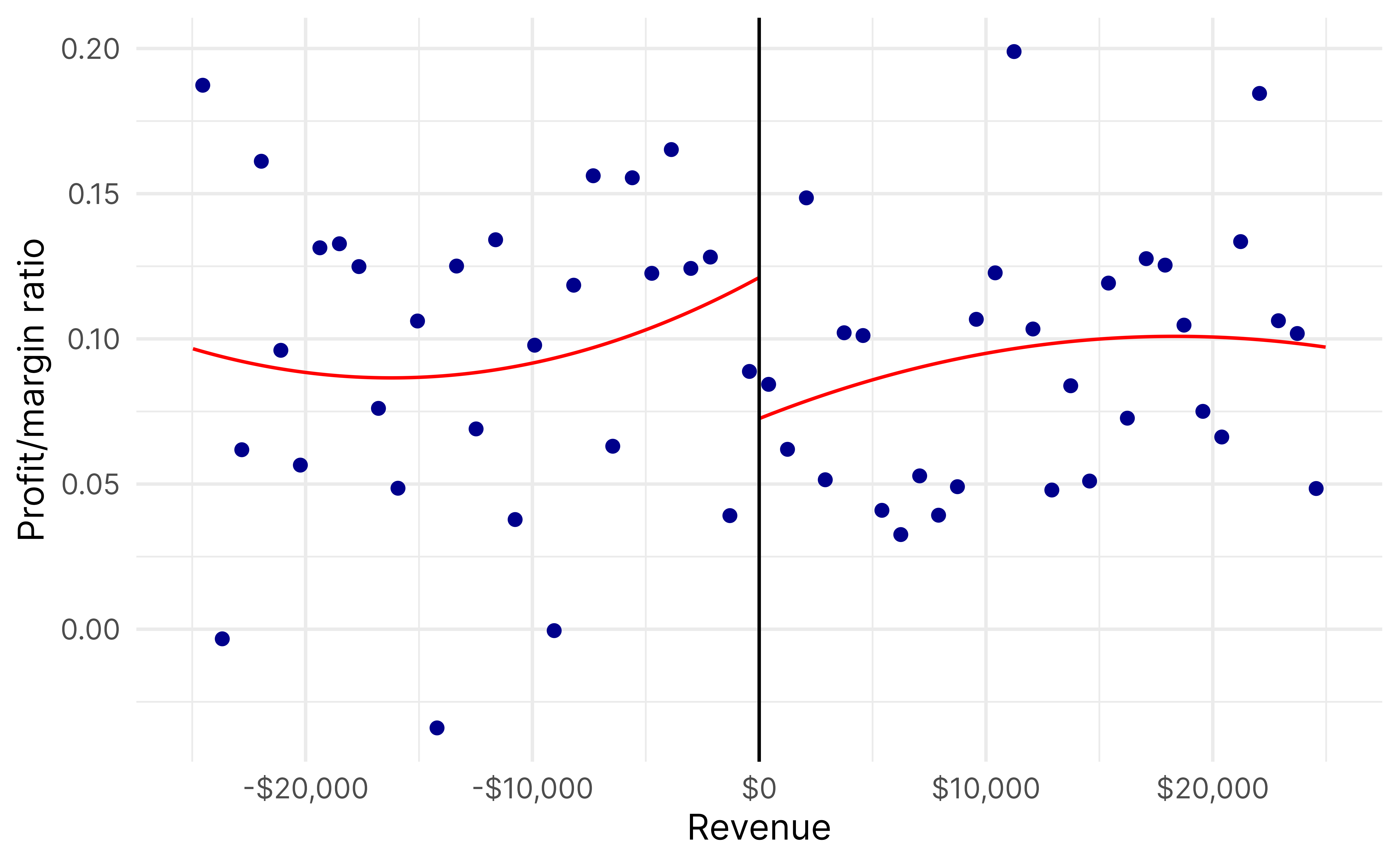
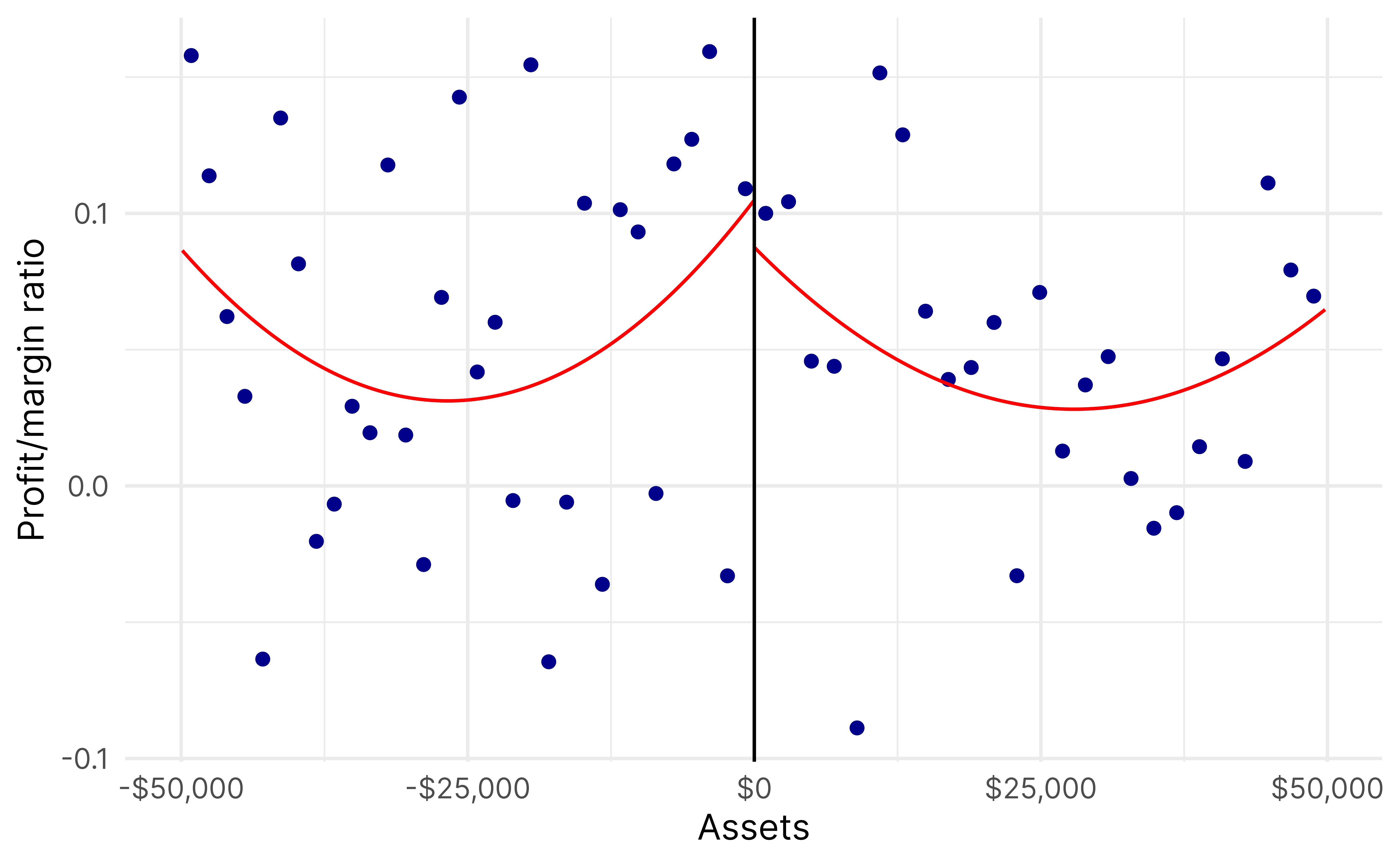
For instance, we can look at organizations around the revenue threshold, but with assets below the asset threshold. This is the vertical line of the L—there’s a lot of variation in asset levels, but everyone has $200,000 ± some amount in revenue.
rd_frontier_revenue <-rdrobust(y = low_assets_only$profit_margin_ratio,x = low_assets_only$revenue_c,c =0,fuzzy = low_assets_only$ez,p =2)summary(rd_frontier_revenue)## Fuzzy RD estimates using local polynomial regression.## ## Number of Obs. 1478## BW type mserd## Kernel Triangular## VCE method NN## ## Number of Obs. 751 727## Eff. Number of Obs. 145 131## Order est. (p) 2 2## Order bias (q) 3 3## BW est. (h) 4117.115 4117.115## BW bias (b) 9375.850 9375.850## rho (h/b) 0.439 0.439## Unique Obs. 736 714## ## First-stage estimates.## ## =============================================================================## Method Coef. Std. Err. z P>|z| [ 95% C.I. ] ## =============================================================================## Conventional -0.360 0.157 -2.286 0.022 [-0.668 , -0.051] ## Robust - - -2.244 0.025 [-0.681 , -0.046] ## =============================================================================## ## Treatment effect estimates.## ## =============================================================================## Method Coef. Std. Err. z P>|z| [ 95% C.I. ] ## =============================================================================## Conventional 0.216 0.243 0.890 0.373 [-0.260 , 0.692] ## Robust - - 0.898 0.369 [-0.263 , 0.708] ## =============================================================================rdplot(y = low_assets_only$profit_margin_ratio,x = low_assets_only$revenue_c,c =0,p =2,hide =TRUE)$rdplot +labs(x ="Revenue", y ="Profit/margin ratio", title =NULL) +scale_x_continuous(labels =label_dollar()) +theme_minimal(base_family ="Inter")
And here’s the vertical part of the L, where everyone has roughly the same assets and everyone has less than $200,000 in revenue:
For instance, we can look at organizations around the revenue threshold, but with assets below the asset threshold. This is the vertical line of the L—there’s a lot of variation in asset levels, but everyone has $200,000 ± some amount in revenue.
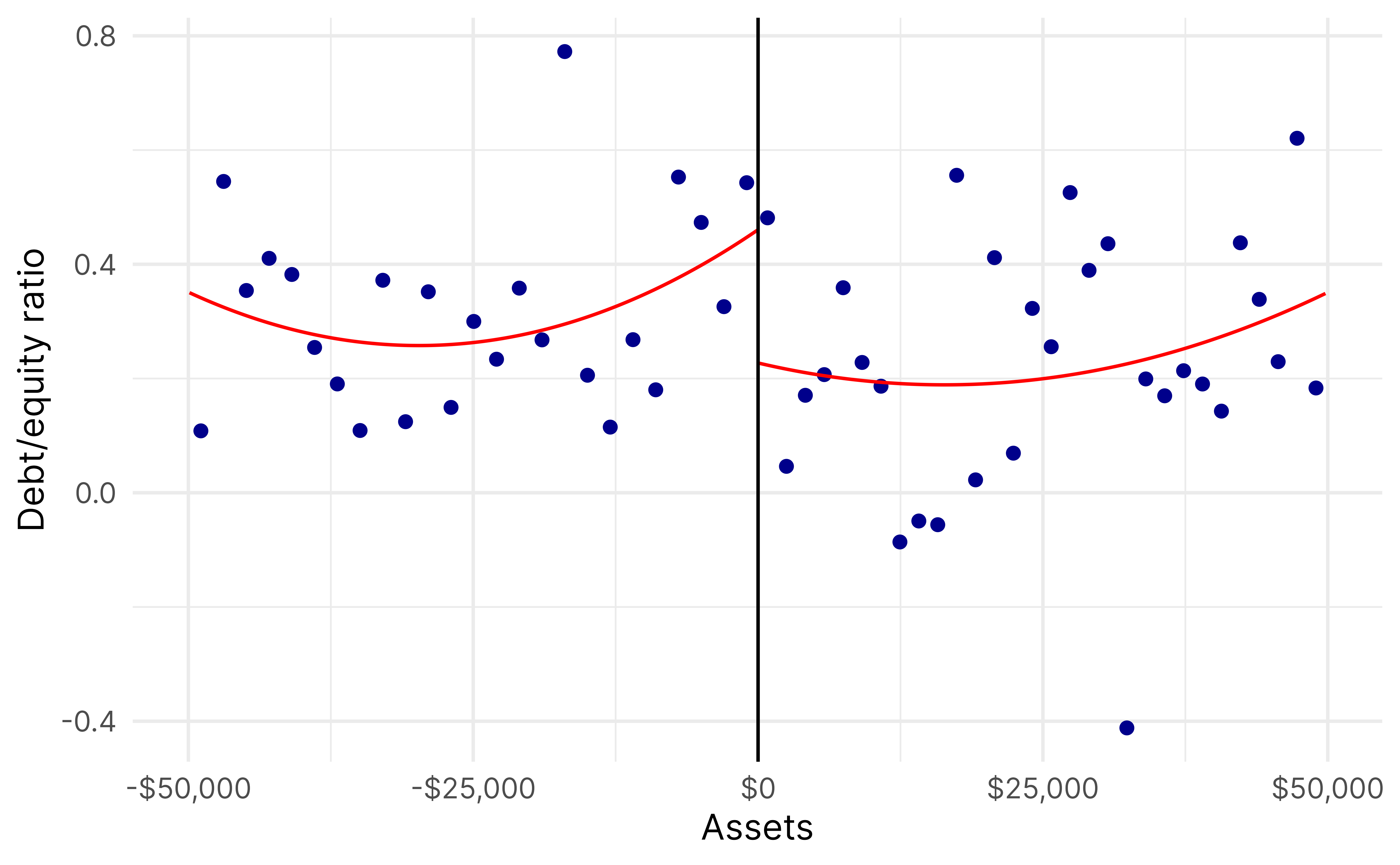
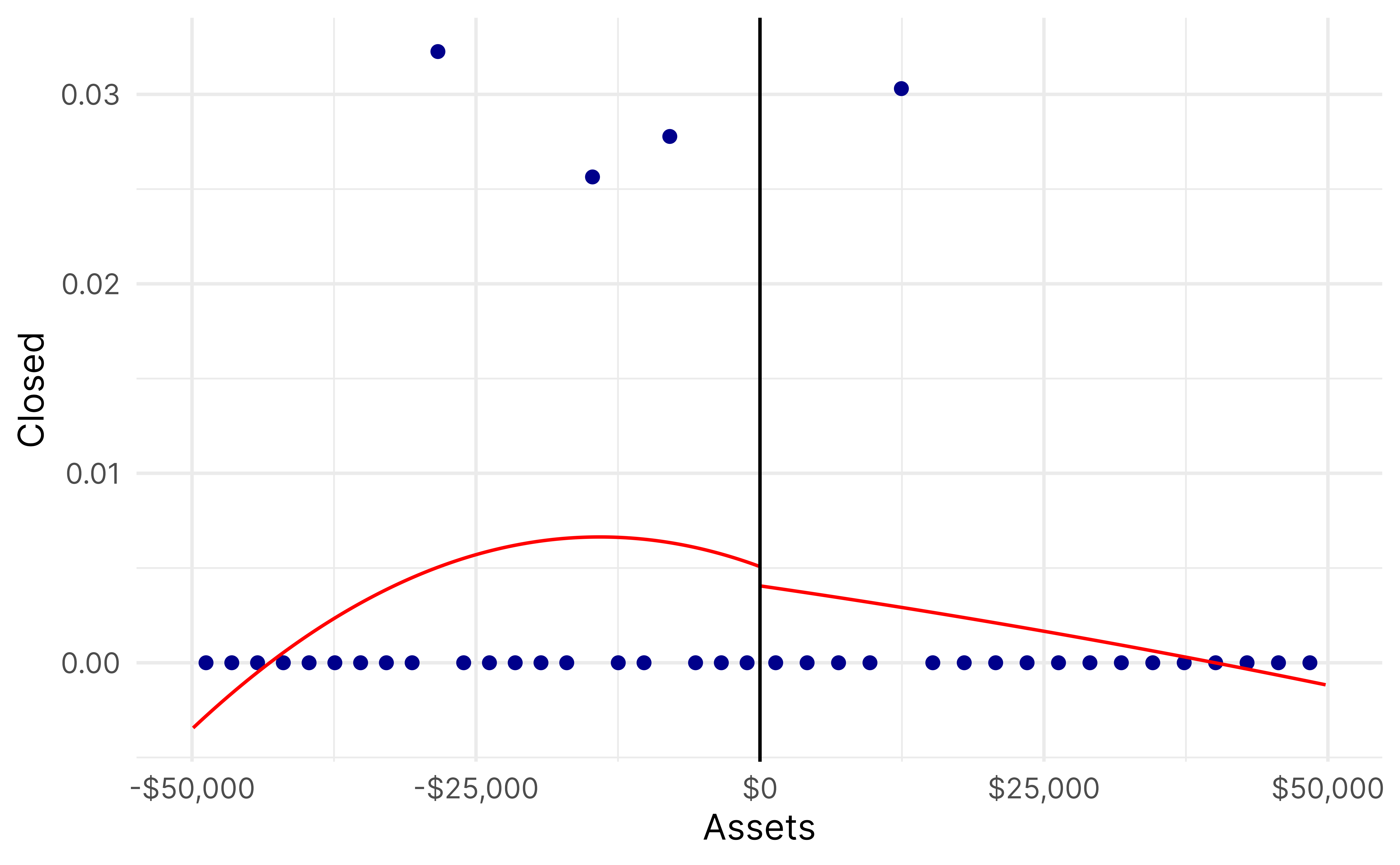
rd_frontier_assets <-rdrobust(y = low_revenue_only$profit_margin_ratio,x = low_revenue_only$assets_c,c =0,fuzzy = low_revenue_only$ez,p =2)summary(rd_frontier_assets)## Fuzzy RD estimates using local polynomial regression.## ## Number of Obs. 1294## BW type mserd## Kernel Triangular## VCE method NN## ## Number of Obs. 708 586## Eff. Number of Obs. 86 74## Order est. (p) 2 2## Order bias (q) 3 3## BW est. (h) 6367.454 6367.454## BW bias (b) 21235.398 21235.398## rho (h/b) 0.300 0.300## Unique Obs. 699 584## ## First-stage estimates.## ## =============================================================================## Method Coef. Std. Err. z P>|z| [ 95% C.I. ] ## =============================================================================## Conventional -0.615 0.150 -4.104 0.000 [-0.909 , -0.321] ## Robust - - -4.096 0.000 [-0.912 , -0.322] ## =============================================================================## ## Treatment effect estimates.## ## =============================================================================## Method Coef. Std. Err. z P>|z| [ 95% C.I. ] ## =============================================================================## Conventional 0.130 0.198 0.655 0.512 [-0.258 , 0.517] ## Robust - - 0.639 0.523 [-0.263 , 0.517] ## =============================================================================rdplot(y = low_revenue_only$profit_margin_ratio,x = low_revenue_only$assets_c,c =0,p =2,hide =TRUE)$rdplot +labs(x ="Assets", y ="Profit/margin ratio", title =NULL) +scale_x_continuous(labels =label_dollar()) +theme_minimal(base_family ="Inter")
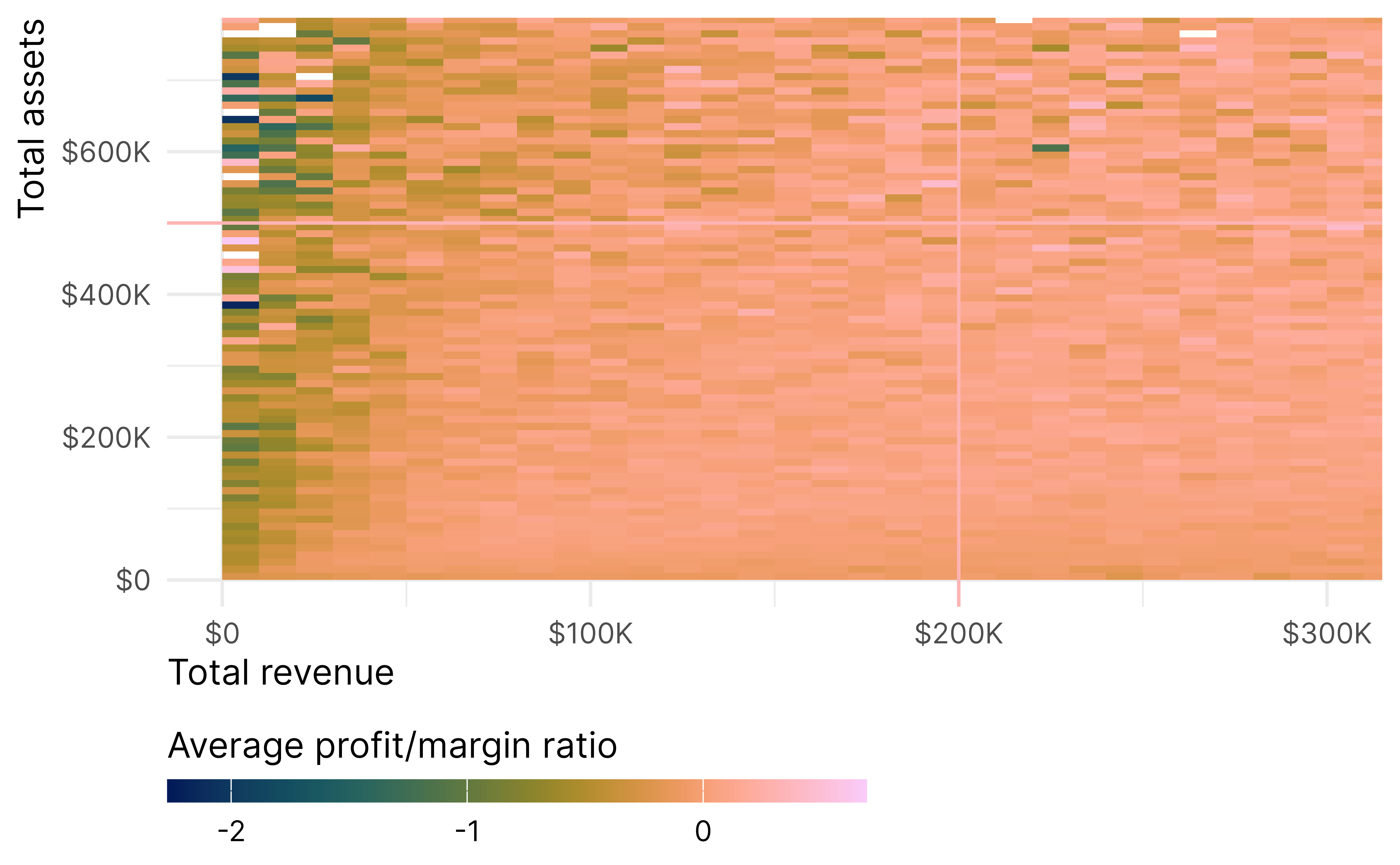
Response surface RD
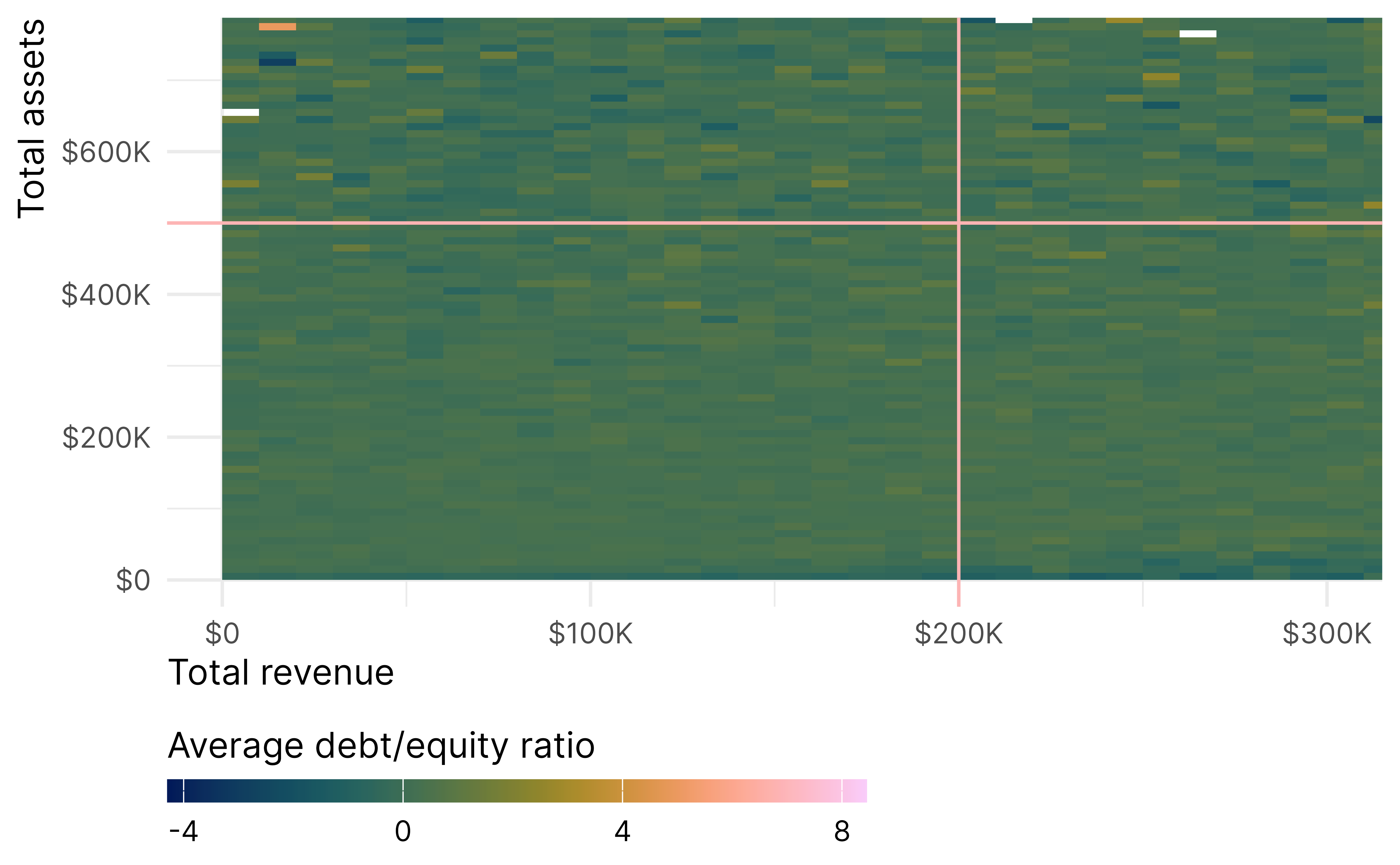
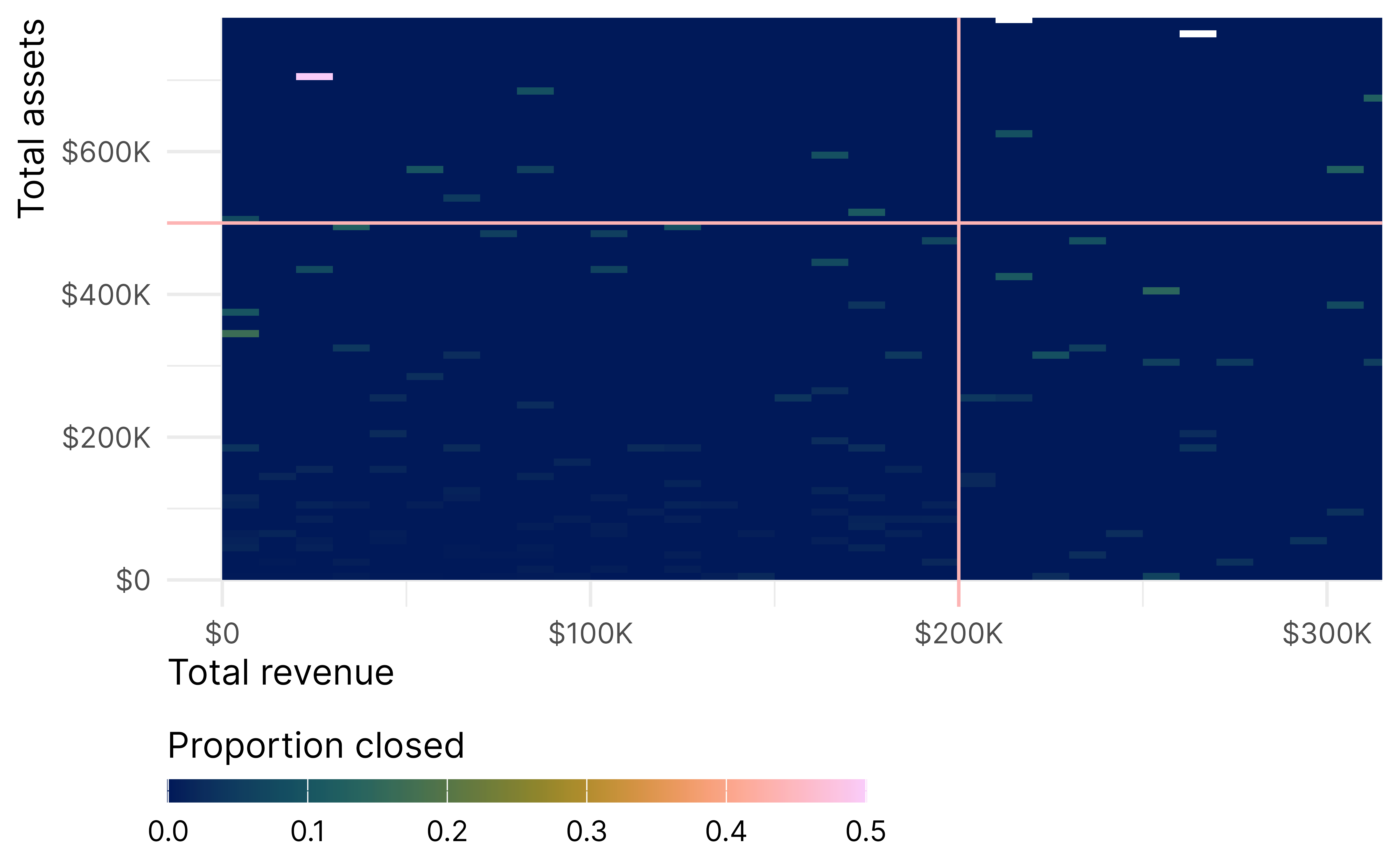
Another alternative is to look at the whole L simultaneously. Reardon and Robinson (2012) call this area the “response surface”. This is tricky to conceptualize because there are multiple dimensions—like the 3D plot earlier of treatment status, revenue and assets create a step or cliff along the L-shaped boundary, were the z-axis is the outcome (rather than probability of treatment that we saw earlier). The response surface RD estimates the height of this cliff.
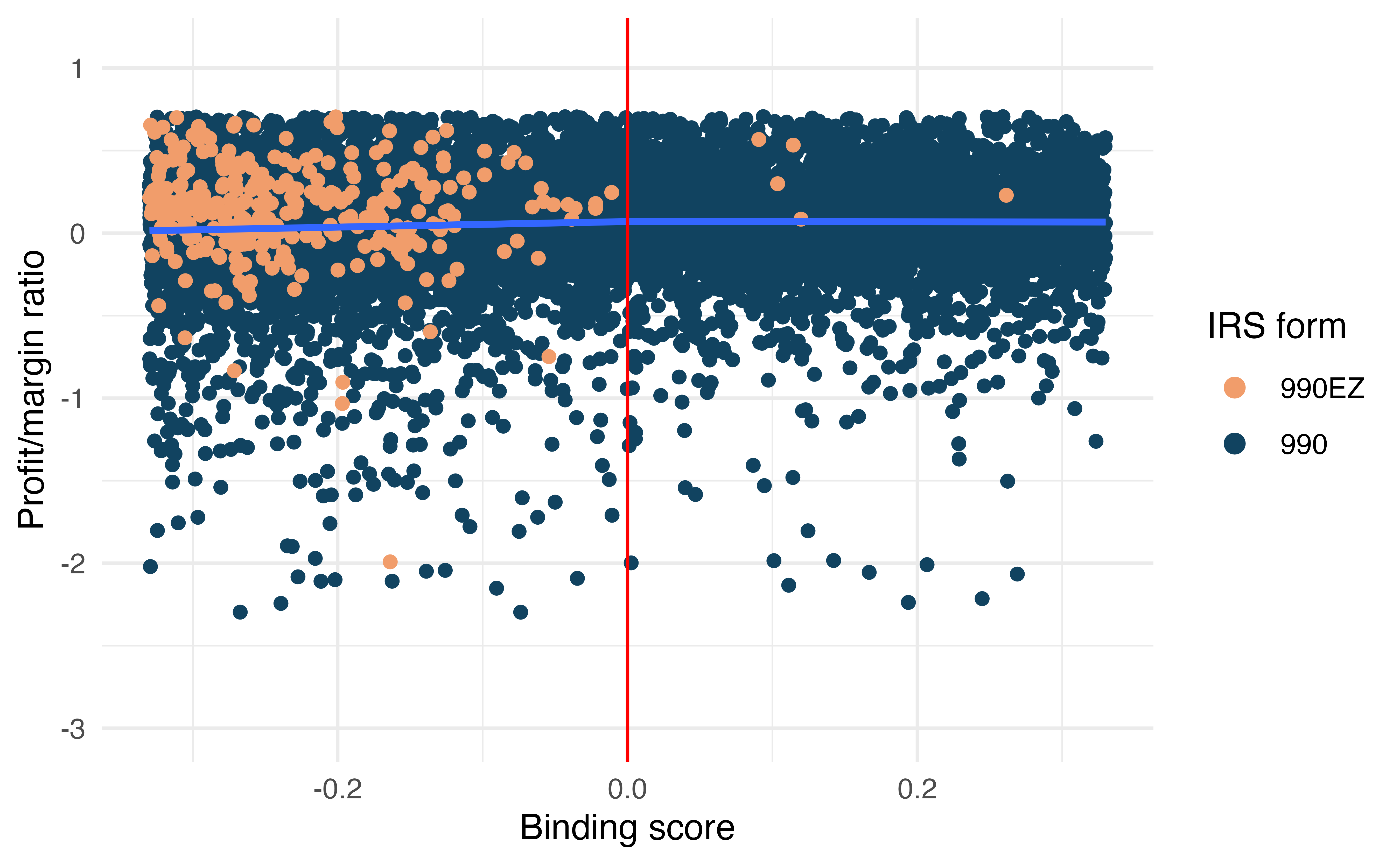
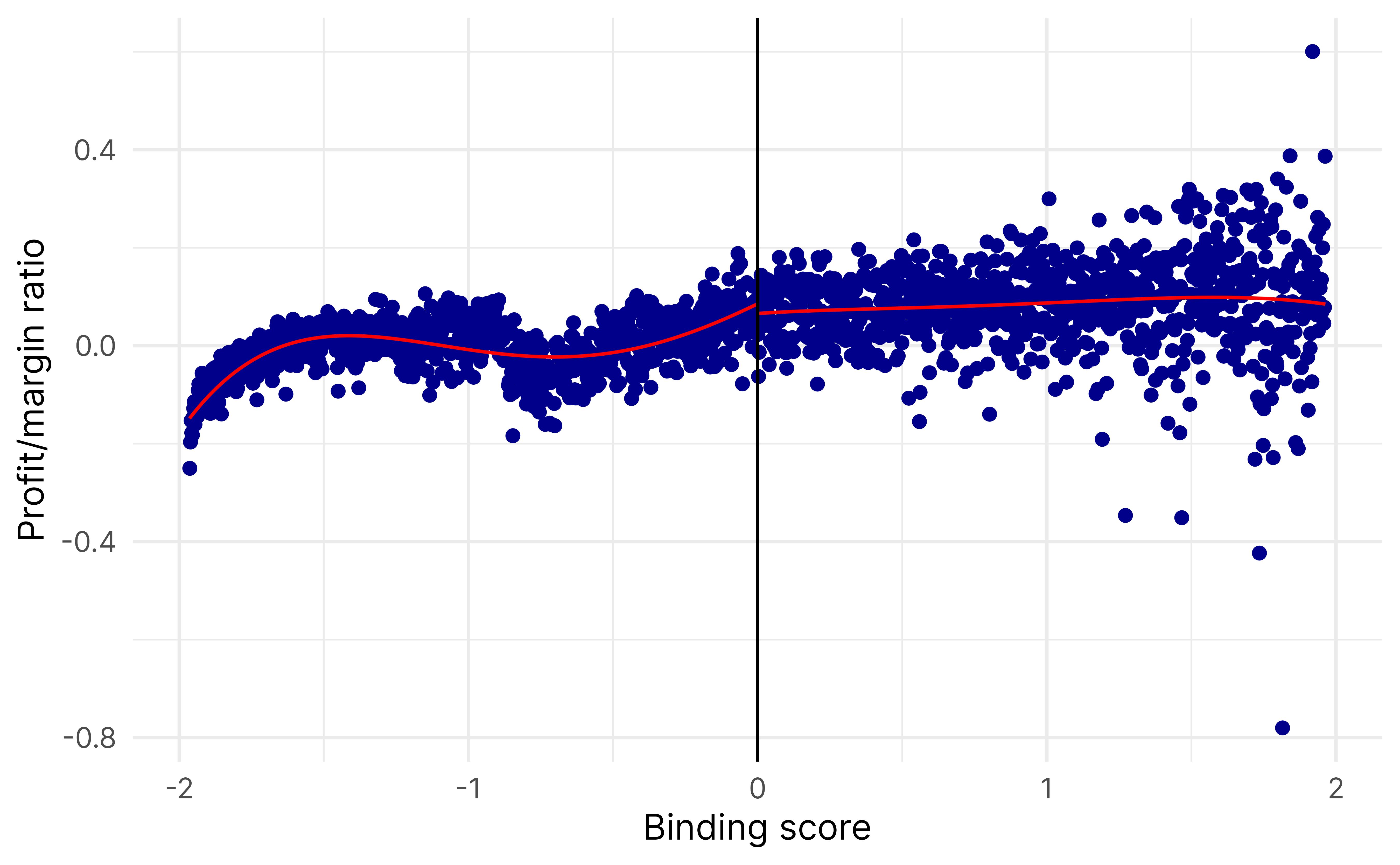
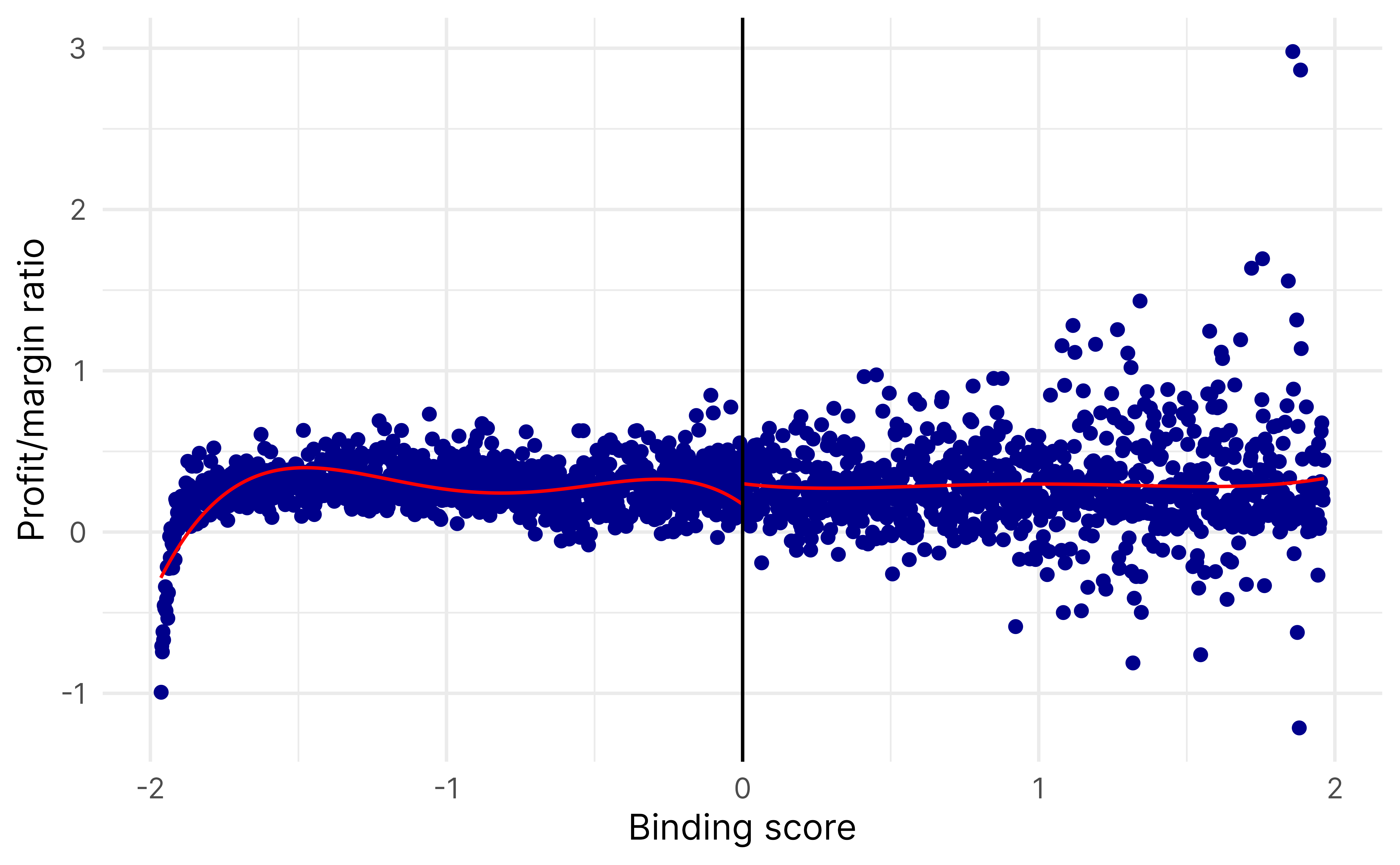
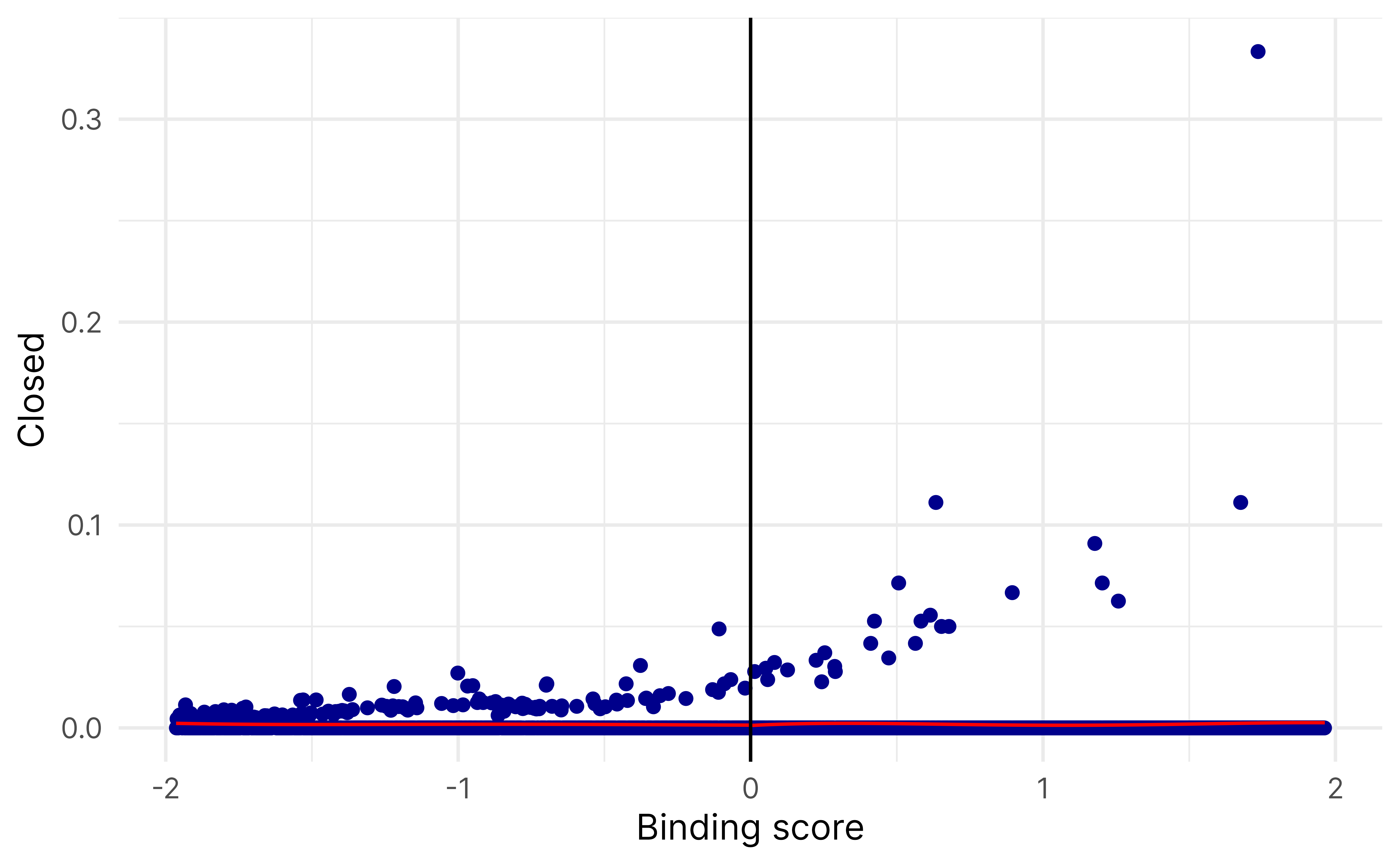
The binding score identifies which standardized running variables is the “binding constraint” and is the minimum of the two standardized scores. It shows:
Which threshold (revenue or assets) is relatively closer to being crossed
How far away the observation is from treatment eligibility
A negative binding score means the observation is eligible for treatment (both revenue and assets are below their thresholds).
The distance score measures the minimum perpendicular distance to the treatment boundary, with sign determined by treatment status. it shows:
How close an observation is to changing treatment status
The sign indicates which side of the boundary the observation falls on
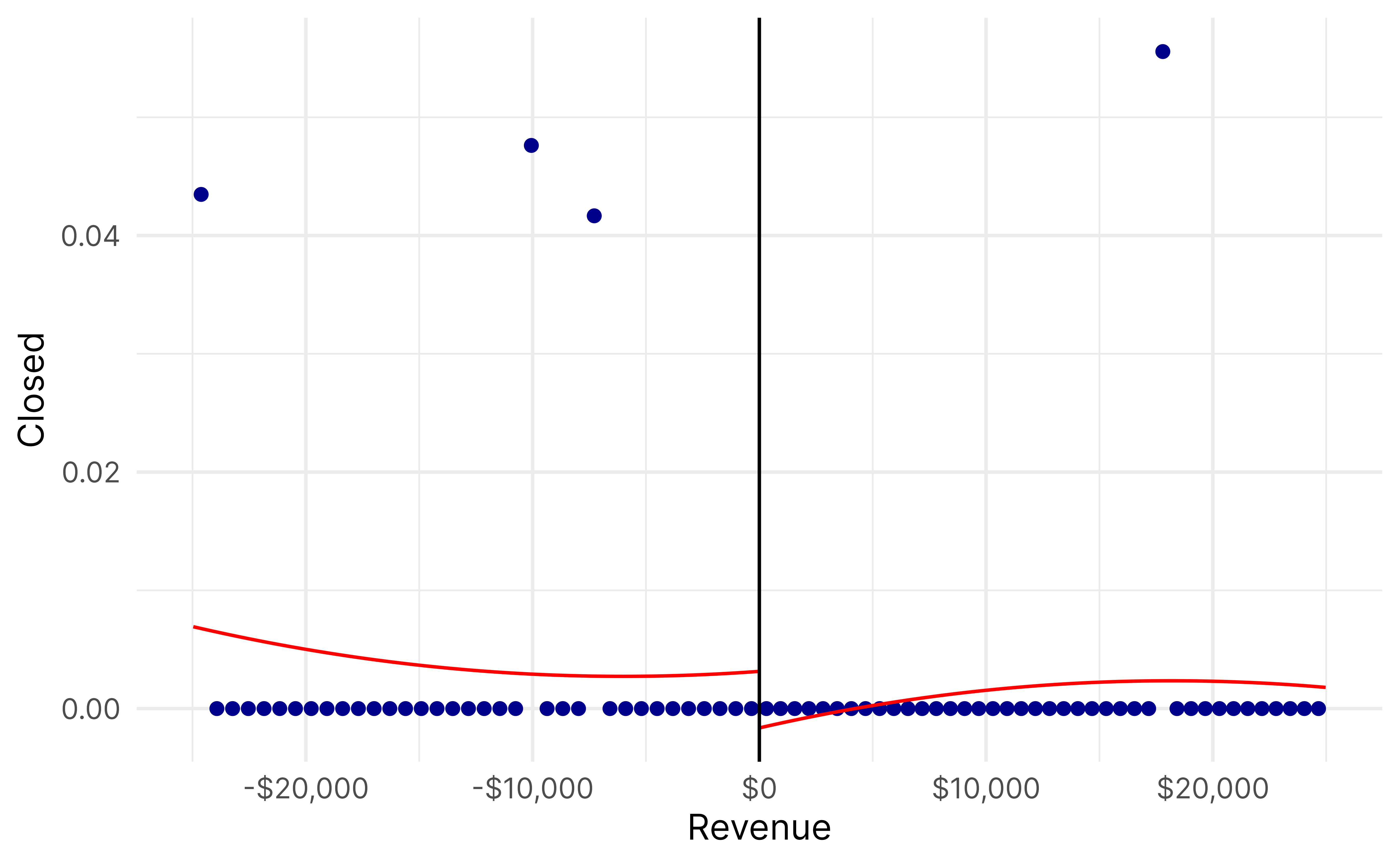
rdrobust(y = binding_data$closed,x = binding_data$binding_score,c =0,fuzzy = binding_data$ez) |>summary()## Fuzzy RD estimates using local polynomial regression.## ## Number of Obs. 119806## BW type mserd## Kernel Triangular## VCE method NN## ## Number of Obs. 104699 15107## Eff. Number of Obs. 2919 2376## Order est. (p) 1 1## Order bias (q) 2 2## BW est. (h) 0.138 0.138## BW bias (b) 0.447 0.447## rho (h/b) 0.309 0.309## Unique Obs. 92277 14949## ## First-stage estimates.## ## =============================================================================## Method Coef. Std. Err. z P>|z| [ 95% C.I. ] ## =============================================================================## Conventional -0.006 0.003 -1.926 0.054 [-0.013 , 0.000] ## Robust - - -2.033 0.042 [-0.014 , -0.000] ## =============================================================================## ## Treatment effect estimates.## ## =============================================================================## Method Coef. Std. Err. z P>|z| [ 95% C.I. ] ## =============================================================================## Conventional -0.247 0.399 -0.620 0.535 [-1.030 , 0.535] ## Robust - - -0.542 0.588 [-1.032 , 0.585] ## =============================================================================
References
Cattaneo, Matias D., Luke Keele, Rocío Titiunik, and Gonzalo Vazquez-Bare. 2016. “Interpreting Regression Discontinuity Designs with Multiple Cutoffs.”The Journal of Politics 78 (4): 1229–48. https://doi.org/10.1086/686802.
———. 2021. “Extrapolating Treatment Effects in Multi-Cutoff Regression Discontinuity Designs.”Journal of the American Statistical Association 116 (536): 1941–52. https://doi.org/10.1080/01621459.2020.1751646.
Reardon, Sean F., and Joseph P. Robinson. 2012. “Regression Discontinuity Designs with Multiple Rating-Score Variables.”Journal of Research on Educational Effectiveness 5 (1): 83–104. https://doi.org/10.1080/19345747.2011.609583.
Source Code
---title: "Playground"---```{r}#| label: setup#| include: falseknitr::opts_chunk$set(fig.width =6,fig.height =6*0.618,fig.retina =3,dev ="ragg_png",fig.align ="center",out.width ="90%",collapse =TRUE,cache.extra =1234# Change number to invalidate cache)options(digits =4,width =300,dplyr.summarise.inform =FALSE)``````{r}#| label: libraries-data#| warning: false#| message: false#| code-fold: truelibrary(tidyverse)library(scales)library(scico)library(fixest)library(rdrobust)library(rdmulti)library(parameters)df_2021 <-readRDS(here::here("data/clean_2021.rds")) |>mutate(revenue_c = revenue -200000,assets_c = assets -500000,eligible = revenue <200000& assets <500000 )clrs <- scico::scico(7, palette ="batlow", categorical =TRUE)```# Discontinuities in running variables## Two running variablesFor a nonprofit to file a 990-EZ, it has to meet two conditions:1. Have gross receipts (revenue) less than $200,000 annually2. Have less than $500,000 in assetsThis creates a situation where we have two running variables, or a bivariate score [@CattaneoKeeleTitiunik:2021; @CattaneoKeeleTitiunik:2016; @Matsudaira:2008] or multiple rating score [@ReardonRobinson:2012].## L-shaped zoneFor causal inference purposes, we look at comparable nonprofts within a narrow bandwidth around the cutoff, but we have to look at both cutoffs simultaneously, creating this L-shape—organizations below and to the left of the two boundaries are treated, while organizations above and to the right are untreated. ```{r}#| warning: false#| message: false#| code-fold: truedf_2021 |>arrange(ez) |># plot the false points first so they don't cover up the truesggplot(aes(x = revenue, y = assets)) +geom_point(aes(color = form), alpha =0.15, size =0.005) +annotate(geom ="segment",x =0,xend =200000,y =500000,color = clrs[7],linewidth =7,alpha =0.75 ) +annotate(geom ="segment",x =0,xend =200000,y =500000,color ="white",linewidth =0.5,alpha =1 ) +annotate(geom ="segment",x =200000,y =0,yend =500000,color = clrs[7],linewidth =7,alpha =0.75 ) +annotate(geom ="segment",x =200000,y =0,yend =500000,color ="white",linewidth =0.5,alpha =1 ) +# geom_label(# data = focus_areas,# aes(label = label),# label.r = unit(0.6, "lines"),# family = "Inter",# fontface = "bold"# ) +scale_x_continuous(labels =label_dollar(scale_cut =cut_short_scale())) +scale_y_continuous(labels =label_dollar(scale_cut =cut_short_scale())) +scale_color_manual(values =c(clrs[5], clrs[6]),guide =guide_legend(override.aes =list(size =2.5, alpha =1)) ) +labs(x ="Total revenue",y ="Total assets",color ="IRS form" ) +coord_cartesian(xlim =c(0, 300000), ylim =c(0, 750000)) +theme_minimal(base_family ="Inter") +theme(axis.title.x =element_text(hjust =0),axis.title.y =element_text(hjust =1),legend.position ="bottom",legend.justification ="left",legend.title.position ="left",legend.margin =margin(l =0, t =0) )```## Fuzzy compliance!Further complicating things, there is substantial imperfect compliance. Not every eligible nonprofit files a 990-EZ, and some that shouldn't qualify file one anyway. For instance, among organizations that were at most $100,000 below the asset threshold, only 43% filed a 990-EZ. 57% could have but didn't.```{r}df_2021 |>filter(assets >400000& assets <500000) |>count(ez, low_revenue = revenue <200000) |>group_by(low_revenue) |>mutate(prop = n /sum(n))```We can visualize that fuzzy noncompliance:```{r}#| warning: false#| message: false#| code-fold: truebucket_size <-25000heatmap_data <- df_2021 |>mutate(revenue_bucket =floor(revenue / bucket_size) * bucket_size,assets_bucket =floor(assets / bucket_size) * bucket_size ) |>group_by(revenue_bucket, assets_bucket) |>summarize(proportion_treated =mean(ez ==TRUE)) |># geom_tile plots from the center of each bucket, so shift these over a bitmutate(revenue_bucket = revenue_bucket + (bucket_size /2),assets_bucket = assets_bucket + (bucket_size /2) )ggplot( heatmap_data,aes(x = revenue_bucket, y = assets_bucket, fill = proportion_treated)) +geom_tile() +geom_vline(xintercept =200000, color = clrs[7]) +geom_hline(yintercept =500000, color = clrs[7]) +scale_fill_scico(palette ="batlow",labels =label_percent(),guide =guide_colorbar(barwidth =15, barheight =0.5) ) +scale_x_continuous(labels =label_dollar(scale_cut =cut_short_scale())) +scale_y_continuous(labels =label_dollar(scale_cut =cut_short_scale())) +labs(x ="Total revenue",y ="Total assets",fill ="% filed 990-EZ" ) +coord_cartesian(xlim =c(0, 300000), ylim =c(0, 750000)) +theme_minimal(base_family ="Inter") +theme(axis.title.x =element_text(hjust =0),axis.title.y =element_text(hjust =1),legend.position ="bottom",legend.justification ="left",legend.title.position ="top",legend.margin =margin(l =0, t =0) )```And with a 3D plot because why not (and because @Matsudaira:2008 did).```{r}#| warning: false#| message: false#| code-fold: truelibrary(plotly)tiny_bucket_size <-10000plot_heatmap_data <- df_2021 |>filter(revenue <300000, assets <750000) |>mutate(revenue_bucket =floor(revenue / tiny_bucket_size) * tiny_bucket_size,assets_bucket =floor(assets / tiny_bucket_size) * tiny_bucket_size ) |>group_by(revenue_bucket, assets_bucket) |>summarize(proportion_treated =mean(ez ==TRUE))plot_ly(data = plot_heatmap_data,x =~revenue_bucket, y =~assets_bucket, z =~proportion_treated,type ="mesh3d",intensity =~proportion_treated,colors = scico::scico(100, palette ="batlow"),showscale =TRUE,colorbar =list(title ="% filed 990-EZ")) |>layout(scene =list(xaxis =list(title ="Total revenue"),yaxis =list(title ="Total assets"),zaxis =list(title ="% filed 990-EZ") ) )```# Discontinuities in outcome variablesSo, we have to deal with two fuzzy discontinuities simultaneously… somehow… @ReardonRobinson:2012 have 5 suggested approaches dealing with two discontinuities, and each have fuzzy analogues. The [{rdmulti}](https://rdpackages.github.io/rdmulti/) package also supports multiple fuzzy discontinuities for nonparametric estimation.We try three different approaches from @ReardonRobinson:2012 here: frontier RD, response surface RD, and binding score RD.## Frontier RDWith frontier RD, we look at the cutoffs—or each of the lines of the L—in isolation. For instance, we can look at organizations around the revenue threshold, but with assets below the asset threshold. This is the vertical line of the L—there's a lot of variation in asset levels, but everyone has $200,000 ± some amount in revenue. Here's the OLS version:```{r}low_assets_only <- df_2021 |>filter(assets >300000& assets <500000) |>filter(revenue >175000& revenue <225000) |>filter( profit_margin_ratio >=quantile(profit_margin_ratio, 0.025) & profit_margin_ratio <=quantile(profit_margin_ratio, 0.975) )frontier_revenue_ols <-feols( profit_margin_ratio ~ revenue_c +I(revenue_c^2) |0| ez ~ eligible,data = low_assets_only,vcov ="HC1")summary(frontier_revenue_ols)model_parameters(frontier_revenue_ols, verbose =FALSE, keep ="ez")```And the `rdrobust()` version:```{r}rd_frontier_revenue <-rdrobust(y = low_assets_only$profit_margin_ratio,x = low_assets_only$revenue_c,c =0,fuzzy = low_assets_only$ez,p =2)summary(rd_frontier_revenue)rdplot(y = low_assets_only$profit_margin_ratio,x = low_assets_only$revenue_c,c =0,p =2,hide =TRUE)$rdplot +labs(x ="Revenue", y ="Profit/margin ratio", title =NULL) +scale_x_continuous(labels =label_dollar()) +theme_minimal(base_family ="Inter")```And here's the vertical part of the L, where everyone has roughly the same assets and everyone has less than $200,000 in revenue:For instance, we can look at organizations around the revenue threshold, but with assets below the asset threshold. This is the vertical line of the L—there's a lot of variation in asset levels, but everyone has $200,000 ± some amount in revenue. We can do it with OLS:```{r}low_revenue_only <- df_2021 |>filter(revenue >100000& revenue <200000) |>filter(assets >450000& assets <550000) |>filter( profit_margin_ratio >=quantile(profit_margin_ratio, 0.025) & profit_margin_ratio <=quantile(profit_margin_ratio, 0.975) )frontier_assets_ols <-feols( profit_margin_ratio ~ assets_c +I(assets_c^2) |0| ez ~ eligible,data = low_revenue_only,vcov ="HC1")summary(frontier_assets_ols)model_parameters(frontier_assets_ols, verbose =FALSE, keep ="ez")```Or with fancier `rdrobust()` stuff:```{r}#| message: falserd_frontier_assets <-rdrobust(y = low_revenue_only$profit_margin_ratio,x = low_revenue_only$assets_c,c =0,fuzzy = low_revenue_only$ez,p =2)summary(rd_frontier_assets)rdplot(y = low_revenue_only$profit_margin_ratio,x = low_revenue_only$assets_c,c =0,p =2,hide =TRUE)$rdplot +labs(x ="Assets", y ="Profit/margin ratio", title =NULL) +scale_x_continuous(labels =label_dollar()) +theme_minimal(base_family ="Inter")```## Response surface RDAnother alternative is to look at the whole L simultaneously. @ReardonRobinson:2012 call this area the "response surface". This is tricky to conceptualize because there are multiple dimensions—like the 3D plot earlier of treatment status, revenue and assets create a step or cliff along the L-shaped boundary, were the z-axis is the outcome (rather than probability of treatment that we saw earlier). The response surface RD estimates the height of this cliff.```{r}L_bandwidth_area <- df_2021 |>filter(revenue >175000& revenue <225000) |>filter(assets >450000& assets <550000) |>mutate(# Calculate distance to nearest thresholddist_revenue =abs(revenue_c) /50000,dist_assets =abs(assets_c) /100000,dist_to_frontier =pmin(dist_revenue, dist_assets),# Make triangular weightskernel_weight =pmax(0, 1- dist_to_frontier) ) |>filter( profit_margin_ratio >=quantile(profit_margin_ratio, 0.025) & profit_margin_ratio <=quantile(profit_margin_ratio, 0.975) )surface_ols <-feols( profit_margin_ratio ~ revenue_c +I(revenue_c^2) + assets_c +I(assets_c^2) + revenue_c:assets_c |0| ez ~ eligible,data = L_bandwidth_area,weights = L_bandwidth_area$kernel_weight,vcov ="HC1")summary(surface_ols)model_parameters(surface_ols, verbose =FALSE, keep ="ez")```That's really hard to visualize though!```{r}#| warning: false#| message: false#| code-fold: truebucket_size <-10000heatmap_data_outcome <- df_2021 |>filter( profit_margin_ratio >=quantile(profit_margin_ratio, 0.025) & profit_margin_ratio <=quantile(profit_margin_ratio, 0.975) ) |>mutate(revenue_bucket =floor(revenue / bucket_size) * bucket_size,assets_bucket =floor(assets / bucket_size) * bucket_size ) |>group_by(revenue_bucket, assets_bucket) |>summarize(avg_outcome =mean(profit_margin_ratio)) |># geom_tile plots from the center of each bucket, so shift these over a bitmutate(revenue_bucket = revenue_bucket + (bucket_size /2),assets_bucket = assets_bucket + (bucket_size /2) )ggplot( heatmap_data_outcome,aes(x = revenue_bucket, y = assets_bucket, fill = avg_outcome)) +geom_tile() +geom_vline(xintercept =200000, color = clrs[7]) +geom_hline(yintercept =500000, color = clrs[7]) +scale_fill_scico(palette ="batlow",# trans = "sqrt",guide =guide_colorbar(barwidth =15, barheight =0.5) ) +scale_x_continuous(labels =label_dollar(scale_cut =cut_short_scale())) +scale_y_continuous(labels =label_dollar(scale_cut =cut_short_scale())) +labs(x ="Total revenue",y ="Total assets",fill ="Average profit/margin ratio" ) +coord_cartesian(xlim =c(0, 300000), ylim =c(0, 750000)) +theme_minimal(base_family ="Inter") +theme(axis.title.x =element_text(hjust =0),axis.title.y =element_text(hjust =1),legend.position ="bottom",legend.justification ="left",legend.title.position ="top",legend.margin =margin(l =0, t =0) )```We can do this with {rdmulti} too:```{r}df_truncated_outcome <- df_2021 |>filter( profit_margin_ratio >=quantile(profit_margin_ratio, 0.025) & profit_margin_ratio <=quantile(profit_margin_ratio, 0.975) )rd_full_L <-rdms(Y = df_truncated_outcome$profit_margin_ratio,X = df_truncated_outcome$revenue_c,C =0,X2 = df_truncated_outcome$assets_c,C2 =0,zvar = df_truncated_outcome$ez,fuzzy = df_truncated_outcome$ez)```## Binding score RDThe binding score identifies which standardized running variables is the "binding constraint" and is the minimum of the two standardized scores. It shows:1. Which threshold (revenue or assets) is relatively closer to being crossed2. How far away the observation is from treatment eligibilityA negative binding score means the observation is eligible for treatment (both revenue and assets are below their thresholds).The distance score measures the minimum perpendicular distance to the treatment boundary, with sign determined by treatment status. it shows:1. How close an observation is to changing treatment status2. The sign indicates which side of the boundary the observation falls on```{r}binding_data <- df_2021 |>mutate(rev_std = (revenue -200000) /sd(revenue),asset_std = (assets -500000) /sd(assets),binding_score =pmin(rev_std, asset_std),distance_score =pmin(abs(rev_std), abs(asset_std)) * (2*eligible -1) ) |>filter( profit_margin_ratio >=quantile(profit_margin_ratio, 0.025) & profit_margin_ratio <=quantile(profit_margin_ratio, 0.975) )``````{r}#| message: falsebinding_data_window <- binding_data |>arrange(ez) |>filter(abs(binding_score) <0.33)ggplot(binding_data_window, aes(x = binding_score, y = profit_margin_ratio)) +geom_point(aes(color = form)) +geom_smooth(data =filter(binding_data_window, binding_score <0),method ="lm" ) +geom_smooth(data =filter(binding_data_window, binding_score >0),method ="lm" ) +geom_vline(xintercept =0, color ="red") +scale_color_manual(values =c(clrs[5], clrs[6]),guide =guide_legend(override.aes =list(size =2.5, alpha =1)) ) +coord_cartesian(ylim =c(-3, 1.1)) +labs(x ="Binding score", y ="Profit/margin ratio", color ="IRS form") +theme_minimal()rdplot(y = binding_data$profit_margin_ratio,x = binding_data$binding_score,c =0,hide =TRUE)$rdplot +labs(x ="Binding score", y ="Profit/margin ratio", title =NULL) +theme_minimal(base_family ="Inter")rdrobust(y = binding_data$profit_margin_ratio,x = binding_data$binding_score,c =0,fuzzy = binding_data$ez) |>summary()```# LeverageThat was all with profit margin ratio. What about leverage, or debt to income ratio?## Frontier RD```{r}low_assets_only <- df_2021 |>filter(assets >300000& assets <500000) |>filter(revenue >175000& revenue <225000) |>filter( debt_to_equity_ratio >=quantile(debt_to_equity_ratio, 0.025) & debt_to_equity_ratio <=quantile(debt_to_equity_ratio, 0.975) )frontier_revenue_ols <-feols( debt_to_equity_ratio ~ revenue_c +I(revenue_c^2) |0| ez ~ eligible,data = low_assets_only,vcov ="HC1")summary(frontier_revenue_ols)model_parameters(frontier_revenue_ols, verbose =FALSE, keep ="ez")``````{r}rd_frontier_revenue <-rdrobust(y = low_assets_only$debt_to_equity_ratio,x = low_assets_only$revenue_c,c =0,fuzzy = low_assets_only$ez,p =2)summary(rd_frontier_revenue)rdplot(y = low_assets_only$debt_to_equity_ratio,x = low_assets_only$revenue_c,c =0,p =2,hide =TRUE)$rdplot +labs(x ="Revenue", y ="Debt/equity ratio", title =NULL) +scale_x_continuous(labels =label_dollar()) +theme_minimal(base_family ="Inter")``````{r}low_revenue_only <- df_2021 |>filter(revenue >100000& revenue <200000) |>filter(assets >450000& assets <550000) |>filter( debt_to_equity_ratio >=quantile(debt_to_equity_ratio, 0.025) & debt_to_equity_ratio <=quantile(debt_to_equity_ratio, 0.975) )frontier_assets_ols <-feols( debt_to_equity_ratio ~ assets_c +I(assets_c^2) |0| ez ~ eligible,data = low_revenue_only,vcov ="HC1")summary(frontier_assets_ols)model_parameters(frontier_assets_ols, verbose =FALSE, keep ="ez")``````{r}#| message: falserd_frontier_assets <-rdrobust(y = low_revenue_only$debt_to_equity_ratio,x = low_revenue_only$assets_c,c =0,fuzzy = low_revenue_only$ez,p =2)summary(rd_frontier_assets)rdplot(y = low_revenue_only$debt_to_equity_ratio,x = low_revenue_only$assets_c,c =0,p =2,hide =TRUE)$rdplot +labs(x ="Assets", y ="Debt/equity ratio", title =NULL) +scale_x_continuous(labels =label_dollar()) +theme_minimal(base_family ="Inter")```## Response surface RD```{r}L_bandwidth_area <- df_2021 |>filter(revenue >175000& revenue <225000) |>filter(assets >450000& assets <550000) |>mutate(# Calculate distance to nearest thresholddist_revenue =abs(revenue_c) /50000,dist_assets =abs(assets_c) /100000,dist_to_frontier =pmin(dist_revenue, dist_assets),# Make triangular weightskernel_weight =pmax(0, 1- dist_to_frontier) ) |>filter( debt_to_equity_ratio >=quantile(debt_to_equity_ratio, 0.025) & debt_to_equity_ratio <=quantile(debt_to_equity_ratio, 0.975) )surface_ols <-feols( debt_to_equity_ratio ~ revenue_c +I(revenue_c^2) + assets_c +I(assets_c^2) + revenue_c:assets_c |0| ez ~ eligible,data = L_bandwidth_area,weights = L_bandwidth_area$kernel_weight,vcov ="HC1")summary(surface_ols)model_parameters(surface_ols, verbose =FALSE, keep ="ez")``````{r}#| warning: false#| message: false#| code-fold: truebucket_size <-10000heatmap_data_outcome <- df_2021 |>filter( debt_to_equity_ratio >=quantile(debt_to_equity_ratio, 0.025) & debt_to_equity_ratio <=quantile(debt_to_equity_ratio, 0.975) ) |>mutate(revenue_bucket =floor(revenue / bucket_size) * bucket_size,assets_bucket =floor(assets / bucket_size) * bucket_size ) |>group_by(revenue_bucket, assets_bucket) |>summarize(avg_outcome =mean(debt_to_equity_ratio)) |># geom_tile plots from the center of each bucket, so shift these over a bitmutate(revenue_bucket = revenue_bucket + (bucket_size /2),assets_bucket = assets_bucket + (bucket_size /2) )ggplot( heatmap_data_outcome,aes(x = revenue_bucket, y = assets_bucket, fill = avg_outcome)) +geom_tile() +geom_vline(xintercept =200000, color = clrs[7]) +geom_hline(yintercept =500000, color = clrs[7]) +scale_fill_scico(palette ="batlow",# trans = "sqrt",guide =guide_colorbar(barwidth =15, barheight =0.5) ) +scale_x_continuous(labels =label_dollar(scale_cut =cut_short_scale())) +scale_y_continuous(labels =label_dollar(scale_cut =cut_short_scale())) +labs(x ="Total revenue",y ="Total assets",fill ="Average debt/equity ratio" ) +coord_cartesian(xlim =c(0, 300000), ylim =c(0, 750000)) +theme_minimal(base_family ="Inter") +theme(axis.title.x =element_text(hjust =0),axis.title.y =element_text(hjust =1),legend.position ="bottom",legend.justification ="left",legend.title.position ="top",legend.margin =margin(l =0, t =0) )``````{r}df_truncated_outcome <- df_2021 |>filter( debt_to_equity_ratio >=quantile(debt_to_equity_ratio, 0.025) & debt_to_equity_ratio <=quantile(debt_to_equity_ratio, 0.975) )rd_full_L <-rdms(Y = df_truncated_outcome$debt_to_equity_ratio,X = df_truncated_outcome$revenue_c,C =0,X2 = df_truncated_outcome$assets_c,C2 =0,zvar = df_truncated_outcome$ez,fuzzy = df_truncated_outcome$ez)```## Binding score RD```{r}binding_data <- df_2021 |>mutate(rev_std = (revenue -200000) /sd(revenue),asset_std = (assets -500000) /sd(assets),binding_score =pmin(rev_std, asset_std),distance_score =pmin(abs(rev_std), abs(asset_std)) * (2*eligible -1) ) |>filter( debt_to_equity_ratio >=quantile(debt_to_equity_ratio, 0.025) & debt_to_equity_ratio <=quantile(debt_to_equity_ratio, 0.975) )``````{r}#| message: falsebinding_data_window <- binding_data |>arrange(ez) |>filter(abs(binding_score) <0.33)rdplot(y = binding_data$debt_to_equity_ratio,x = binding_data$binding_score,c =0,hide =TRUE)$rdplot +labs(x ="Binding score", y ="Profit/margin ratio", title =NULL) +theme_minimal(base_family ="Inter")rdrobust(y = binding_data$debt_to_equity_ratio,x = binding_data$binding_score,c =0,fuzzy = binding_data$ez) |>summary()```# SurvivalHow about survival? This is tricky since there aren't a ton of closings:```{r}df_2021 |>count(closed, eligible)```But we try regardless!## Frontier RD```{r}low_assets_only <- df_2021 |>filter(assets >300000& assets <500000) |>filter(revenue >175000& revenue <225000)frontier_revenue_ols <-feols( closed ~ revenue_c +I(revenue_c^2) |0| ez ~ eligible,data = low_assets_only,vcov ="HC1")summary(frontier_revenue_ols)model_parameters(frontier_revenue_ols, verbose =FALSE, keep ="ez")``````{r}rd_frontier_revenue <-rdrobust(y = low_assets_only$closed,x = low_assets_only$revenue_c,c =0,fuzzy = low_assets_only$ez,p =2)summary(rd_frontier_revenue)rdplot(y = low_assets_only$closed,x = low_assets_only$revenue_c,c =0,p =2,hide =TRUE)$rdplot +labs(x ="Revenue", y ="Closed", title =NULL) +scale_x_continuous(labels =label_dollar()) +theme_minimal(base_family ="Inter")``````{r}low_revenue_only <- df_2021 |>filter(revenue >100000& revenue <200000) |>filter(assets >450000& assets <550000)frontier_assets_ols <-feols( closed ~ assets_c +I(assets_c^2) |0| ez ~ eligible,data = low_revenue_only,vcov ="HC1")summary(frontier_assets_ols)model_parameters(frontier_assets_ols, verbose =FALSE, keep ="ez")``````{r}#| message: falserd_frontier_assets <-rdrobust(y = low_revenue_only$closed,x = low_revenue_only$assets_c,c =0,fuzzy = low_revenue_only$ez,p =2)summary(rd_frontier_assets)rdplot(y = low_revenue_only$closed,x = low_revenue_only$assets_c,c =0,p =2,hide =TRUE)$rdplot +labs(x ="Assets", y ="Closed", title =NULL) +scale_x_continuous(labels =label_dollar()) +theme_minimal(base_family ="Inter")```## Response surface RD```{r}L_bandwidth_area <- df_2021 |>filter(revenue >175000& revenue <225000) |>filter(assets >450000& assets <550000) |>mutate(# Calculate distance to nearest thresholddist_revenue =abs(revenue_c) /50000,dist_assets =abs(assets_c) /100000,dist_to_frontier =pmin(dist_revenue, dist_assets),# Make triangular weightskernel_weight =pmax(0, 1- dist_to_frontier) )surface_ols <-feols( closed ~ revenue_c +I(revenue_c^2) + assets_c +I(assets_c^2) + revenue_c:assets_c |0| ez ~ eligible,data = L_bandwidth_area,weights = L_bandwidth_area$kernel_weight,vcov ="HC1")summary(surface_ols)model_parameters(surface_ols, verbose =FALSE, keep ="ez")``````{r}#| warning: false#| message: false#| code-fold: truebucket_size <-10000heatmap_data_outcome <- df_2021 |>mutate(revenue_bucket =floor(revenue / bucket_size) * bucket_size,assets_bucket =floor(assets / bucket_size) * bucket_size ) |>group_by(revenue_bucket, assets_bucket) |>summarize(avg_outcome =mean(closed ==TRUE)) |># geom_tile plots from the center of each bucket, so shift these over a bitmutate(revenue_bucket = revenue_bucket + (bucket_size /2),assets_bucket = assets_bucket + (bucket_size /2) )ggplot( heatmap_data_outcome,aes(x = revenue_bucket, y = assets_bucket, fill = avg_outcome)) +geom_tile() +geom_vline(xintercept =200000, color = clrs[7]) +geom_hline(yintercept =500000, color = clrs[7]) +scale_fill_scico(palette ="batlow",# trans = "sqrt",guide =guide_colorbar(barwidth =15, barheight =0.5) ) +scale_x_continuous(labels =label_dollar(scale_cut =cut_short_scale())) +scale_y_continuous(labels =label_dollar(scale_cut =cut_short_scale())) +labs(x ="Total revenue",y ="Total assets",fill ="Proportion closed" ) +coord_cartesian(xlim =c(0, 300000), ylim =c(0, 750000)) +theme_minimal(base_family ="Inter") +theme(axis.title.x =element_text(hjust =0),axis.title.y =element_text(hjust =1),legend.position ="bottom",legend.justification ="left",legend.title.position ="top",legend.margin =margin(l =0, t =0) )``````{r}df_truncated_outcome <- df_2021rd_full_L <-rdms(Y = df_truncated_outcome$closed,X = df_truncated_outcome$revenue_c,C =0,X2 = df_truncated_outcome$assets_c,C2 =0,zvar = df_truncated_outcome$ez,fuzzy = df_truncated_outcome$ez)```## Binding score RD```{r}binding_data <- df_2021 |>mutate(rev_std = (revenue -200000) /sd(revenue),asset_std = (assets -500000) /sd(assets),binding_score =pmin(rev_std, asset_std),distance_score =pmin(abs(rev_std), abs(asset_std)) * (2*eligible -1) )``````{r}#| message: falsebinding_data_window <- binding_data |>arrange(ez) |>filter(abs(binding_score) <0.33)rdplot(y = binding_data$closed,x = binding_data$binding_score,c =0,hide =TRUE)$rdplot +labs(x ="Binding score", y ="Closed", title =NULL) +theme_minimal(base_family ="Inter")rdrobust(y = binding_data$closed,x = binding_data$binding_score,c =0,fuzzy = binding_data$ez) |>summary()```# References