Figures and tables in paper
Andrew Heiss
Last run: July 6, 2018
knitr::opts_chunk$set(cache = FALSE, fig.retina = 2,
                      tidy.opts = list(width.cutoff = 120),  # For code
width = 120) # For outputlibrary(tidyverse)
library(pander)
library(countrycode)
library(ggrepel)
library(ggstance)
library(gridExtra)
library(here)
# Load pre-cleaned data
edb_clean <- read_rds(file.path(here(), "output", "data", "edb_clean.rds"))
edb_reforms <- read_rds(file.path(here(), "output", "data", "edb_reforms.rds"))
# Load helpful functions
source(file.path(here(), "lib", "model_stuff.R"))
source(file.path(here(), "lib", "graphics_stuff.R"))Tables
Table 2: Overview of De Jure Reform Measures
Not generated with this script.
Table 3: Summary of Coefficients for 8 OLS Models
Important: All models only use countries included in the original 2001 report.
These difference models use the lag of the outcome variable and a year indicator variable to determine the change in outcome variable.
Formally, this is defined as:
\[ y_t = \beta_0 + \beta_1 y_{t-1} + \beta_2 X + \epsilon \]
- t = Year
- X = {1 if t = cutpoint year, 0 otherwise}
- β0 = Constant
- β1 = Change in outcome from the previous year
- β2 = Effect of the event
Or an example R formula:
sb_proced ~ sb_proced_lag + ranked_2005# Define all the models that need to be run
# For the paper we just do 2005 and 2006 for all countries. In the appendix we
# run models from 2003-2013 for all countries, countries with EDB committees,
# and countries without EDB committees
models_to_run <- expand.grid(year = 2005:2006,
outcome = c("sb_proced", "sb_days_ln",
"sb_cost_ln", "sb_capital_ln"),
grouping = "All countries",
stringsAsFactors = FALSE)
# This function generates an R model formula based on the name of the dependent
# variable and the year provided. i.e., given "sb_proced" and "2005", it will
# create the formula "sb_proced ~ sb_proced_lag + ranked_2005" and run the model
run_lagged_ols_model <- function(outcome, year, df) {
outcome_lag <- paste0(outcome, "_lag")
year_variable <- paste0("ranked_", year)
form <- as.formula(paste0(outcome, " ~ ", outcome_lag, " + ", year_variable))
lm(form, data = df)
}
# Run models only on countries that were included in the 2001 report
models_to_run_full <- edb_clean %>%
filter(in_2001 == 1) %>%
# Add grouping column so this can be joined with models_to_run
mutate(grouping = "All countries") %>%
group_by(grouping) %>%
nest() %>%
right_join(models_to_run, by = "grouping")
# Run all the models within the data frame
ols_models_lagged <- models_to_run_full %>%
mutate(model = pmap(.l = list(outcome, year, data), run_lagged_ols_model),
# Add robust clustered SEs
robust_se = pmap(.l = list(model, data, "ccode"), robust_clusterify),
# Add model summary statistics
glance = model %>% map(broom::glance),
# Add a data frame of model parameters with correct SEs
tidy_robust = robust_se %>% map(~ broom::tidy(.$coef)))
# Extract the ranking coefficients from all models
ols_coefs <- ols_models_lagged %>%
# Spread out the model results
unnest(tidy_robust) %>%
# Only look at the ranked* coefficients
filter(str_detect(term, "ranked")) %>%
# Clean up the estimates, labels, and add stars
mutate(value = paste0(sprintf("%.3f", round(estimate, 3)), p_stars(p.value)),
term = str_replace(term, "\\.\\d+TRUE", "")) %>%
# Get rid of extra columns
select(-c(estimate, std.error, statistic, p.value)) %>%
spread(outcome, value) %>%
# Give table clean column names
select(Subset = grouping, Year = year,
Procedures = sb_proced, `Cost (log)` = sb_cost_ln,
`Days (log)` = sb_days_ln, `Capital (log)` = sb_capital_ln)caption <- 'Summary of β~2~ coefficients (i.e. "ranked_200x") for difference models'
tbl_ols <- pandoc.table.return(filter(ols_coefs, Year %in% c(2005, 2006)),
caption = caption)
cat(tbl_ols)| Subset | Year | Procedures | Cost (log) | Days (log) | Capital (log) |
|---|---|---|---|---|---|
| All countries | 2005 | -0.176** | -0.081*** | -0.040* | -0.030 |
| All countries | 2006 | -0.240*** | -0.071*** | -0.049** | -0.097* |
Table 4: Summary of Coefficients for 8 ITS Models
These interrupted times series models use an interaction term of the years since an intervention and the intervention itself to determine the change in slope after the intervention.
\[ y_t = \beta_0 + \beta_1 T + \beta_2 X_t + \beta_3 (T \times X_t) + \epsilon \]
- t = Year
- T = Years before/after cutpoint
- X = {1 if t = cutpoint year, 0 otherwise}
- β0 = Constant: pre-period intercept - baseline pre intervention
- β1 = pre-period slope - baseline time trend - level of increase prior to intervention
- β2 = immediate effect of the event - change in intercept at point of experiment
- β3 = change in slope after the experiment - what happens after
Or an example R formula:
sb_proced ~ year_centered_2005 + ranked_2005 + year_centered_2005 * ranked_2005# As with run_lagged_ols_model(), this function generates an R model formula and
# runs it. i.e., given "sb_proced" and "2005", it will create the formula
# "sb_proced ~ year_centered_2005 + ranked_2005 + year_centered_2005 * ranked_2005"
# and run the model
run_its_model <- function(outcome, year, df) {
year_variable <- paste0("ranked_", year)
year_centered <- paste0("year_centered_", year)
form <- as.formula(paste0(outcome, " ~ ", year_centered, " + ", year_variable,
" + ", year_centered, " * ", year_variable))
lm(form, data = df)
}
# Run all the ITS models within the data frame
its_models <- models_to_run_full %>%
mutate(model = pmap(.l = list(outcome, year, data), run_its_model),
robust_se = pmap(.l = list(model, data, "ccode"), robust_clusterify),
glance = model %>% map(broom::glance),
tidy_robust = robust_se %>% map(~ broom::tidy(.$coef)))
# Extract the ranking coefficients from ITS models
its_coefs <- its_models %>%
# Spread out the model results
unnest(tidy_robust) %>%
# Only look at the coefficients from interaction terms (they have ":" in their names)
filter(str_detect(term, ":")) %>%
# Clean up the estimates, labels, and add stars
mutate(value = paste0(sprintf("%.3f", round(estimate, 3)), p_stars(p.value)),
term = str_replace(term, "\\.\\d+TRUE", "")) %>%
# Get rid of extra columns
select(-c(estimate, std.error, statistic, p.value)) %>%
spread(outcome, value) %>%
# Give table clean column names
select(Subset = grouping, Year = year,
Procedures = sb_proced, `Cost (log)` = sb_cost_ln,
`Days (log)` = sb_days_ln, `Capital (log)` = sb_capital_ln)caption <- 'Summary of β~3~ coefficients (i.e. "year.centered.200x × ranked.200x")'
tbl_its <- pandoc.table.return(filter(its_coefs, Year %in% c(2005, 2006)),
caption = caption)
cat(tbl_its)| Subset | Year | Procedures | Cost (log) | Days (log) | Capital (log) |
|---|---|---|---|---|---|
| All countries | 2005 | -0.088 | -0.059** | 0.009 | 0.054 |
| All countries | 2006 | -0.105 | -0.041** | 0.008 | -0.019 |
Table 5: Countries with Reform Committees Directly Using the EDB Data
Not generated with this script.
Table 6: Experimental Results Status Comparisons on Importance of EBD and Business Climate Improvements
Not generated with this script.
Table 7: Experimental Results of Ranking Differences on Investment Likelihood
Not generated with this script.
Figures
Figure 1: Doing Business Website Visits, Annually (2003-2016)
Estimated data based on a screenshot of internal EDB web traffic reports.
edb_web <- read_csv(file.path(here(), "data_raw", "edb-traffic_2013-2016.csv"),
                    col_names = c("Year", "Visits"))

fig_edb_web <- ggplot(edb_web, aes(x = Year, y = Visits)) +
  geom_line() +
  labs(x = NULL, y = "Annual visits") +
  scale_y_continuous(labels = scales::comma) +
  scale_x_continuous(breaks = seq(2002, 2016, 2)) +
  theme_edb() +
  theme(panel.grid.minor = element_blank())

fig_edb_web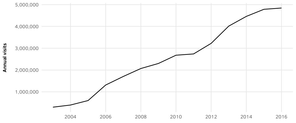
ggsave(fig_edb_web,
       filename = file.path(here(), "output", "figures", "edb_website_traffic.pdf"),
       width = 6, height = 2.5, units = "in", device = cairo_pdf)
ggsave(fig_edb_web,
       filename = file.path(here(), "output", "figures", "edb_website_traffic.png"),
       width = 6, height = 2.5, units = "in", type = "cairo", dpi = 300)
Figure 2: Average change in select subindicators, before and after public ranking (2006)
df_plot_edb_2001 <- edb_clean %>%
  # Only look at countries in the 2001 report
  filter(in_2001 == 1) %>%
  select(year, sb_days, sb_proced, sb_cost, sb_capital, con_days, con_proced) %>%
  # Calculate average of each variable by year
  gather(variable, value, -year) %>%
  group_by(year, variable) %>%
  summarise(avg = mean(value, na.rm = TRUE)) %>%
  filter(!is.nan(avg)) %>%
  # Only use 2004 and beyond
  filter(year >= 2003) %>%
  mutate(variable = fct_recode(variable,
                               `Contract—Days` = "con_days",
                               `Contract—Procedures` = "con_proced",
                               `Starting a business—Capital` = "sb_capital",
                               `Starting a business—Cost` = "sb_cost",
                               `Starting a business—Days` = "sb_days",
                               `Starting a business—Procedures` = "sb_proced"))

# Mark the intervention years
plot_interventions <- data_frame(year = 2005:2006,
                                 intervention = c("2005", "2006"))

# Technically, facets in gpplot are for different aspects of the same value, not
# for separate variables. This function creates a miniature ggplot object which
# then gets combined below with gridExtra::arrangeGrob()
make_faux_facet <- function(x, ymin, ymax, ylab) {
  plot_data <- df_plot_edb_2001 %>%
    filter(variable == x)

  faux_facet <- ggplot() +
    geom_vline(data = plot_interventions, aes(xintercept = year,
                                            colour = intervention),
               linetype = "dashed", size = 0.5) +
    geom_line(data = plot_data, aes(x = year, y = avg)) +
    scale_color_manual(values = c(its_1, its_2), name = NULL) +
    scale_x_continuous(limits = c(2000, 2015), breaks = seq(2000, 2015, 5)) +
    coord_cartesian(xlim = c(2000, 2015), ylim = c(ymin, ymax)) +
    guides(color = FALSE) +
    labs(x = NULL, y = ylab, title = x) +
    theme_edb() +
    theme(plot.title = element_text(size = rel(1), hjust = 0.5))

  return(faux_facet)
}

# Create a data frame with plotting parameters and then create ggplot objects in a new column
plots_2001 <- tribble(
  ~ymin, ~ymax, ~ylab,        ~variable,
  0,     610,   "Days",       "Contract—Days",
  0,     45,    "Procedures", "Contract—Procedures",
  0,     200,   "Capital",    "Starting a business—Capital",
  0,     100,   "Cost",       "Starting a business—Cost",
  0,     50,    "Days",       "Starting a business—Days",
  0,     10,    "Procedures", "Starting a business—Procedures"
) %>%
  mutate(facet = pmap(.l = list(variable, ymin, ymax, ylab), make_faux_facet))

# Plot all those plots in one big mega plot
plot_edb_2001 <- arrangeGrob(grobs = plots_2001$facet, nrow = 2)
grid::grid.newpage()
grid::grid.draw(plot_edb_2001)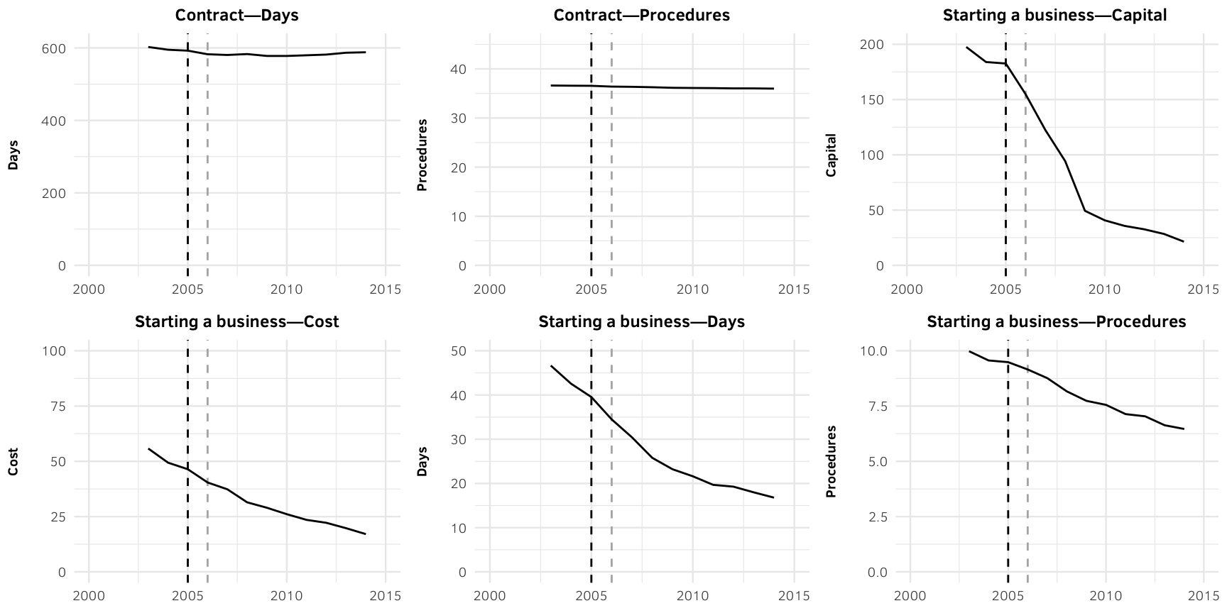
ggsave(plot_edb_2001,
       filename = file.path(here(), "output", "figures", "edb_its_2001.pdf"),
       width = 9, height = 4.5, units = "in", device = cairo_pdf)
ggsave(plot_edb_2001,
       filename = file.path(here(), "output", "figures", "edb_its_2001.png"),
       width = 9, height = 4.5, units = "in", type = "cairo", dpi = 300)
Figure 3: EDB Rankings, 2005 versus 2014, by Committee Status Based on 2015 report
# Select only 2005 and 2014 rankings
edb_rankings <- edb_clean %>%
  select(ccode, year, p_edb_rank, has_bureau) %>%
  filter(year %in% c(2005, 2014)) %>%
  spread(year, p_edb_rank) %>%
  mutate(countryname = countrycode(ccode, "cown", "country.name"),
         countryname = ifelse(countryname == "Lao People's Democratic Republic",
                              "Laos", countryname),
         add_label = countryname %in% c("Georgia", "Rwanda",
                                        "Bangladesh", "Nigeria", "Pakistan",
                                        "Norway", "New Zealand",
                                        "Laos", "Niger"),
         label = ifelse(add_label, countryname, NA))

# Extra stuff that will go on the plot
annotations <- data_frame(x = c(max(edb_rankings$`2005`, na.rm = TRUE), 0),
                          y = c(0, max(edb_rankings$`2014`, na.rm = TRUE)),
                          text = c("Outliers\nimproving", "Outliers\nworsening"),
                          hjust = c("right", "left"),
                          vjust = c("bottom", "top"))

reference_line <- data_frame(x = c(0, max(edb_rankings$`2005`, na.rm = TRUE)),
                             y = c(0, max(edb_rankings$`2014`, na.rm = TRUE)))

# Set the seed every time geom_label_repel is called so the labels are repositioned the same way
set.seed(1234)
fig_rankings_corr <- ggplot(edb_rankings, aes(x = `2005`, y = `2014`,
                                              colour = has_bureau, label = label)) +
  # geom_smooth(aes(fill = has_bureau), method = "lm", size = 0.5, alpha = 0.1, fullrange = TRUE) +
  geom_line(data = reference_line, aes(x = x, y = y, label = NULL), colour = "grey70", size = 0.5) +
  geom_point(size = 1) +
  geom_label_repel(aes(fill = has_bureau), colour = "white",
                   size = 2, alpha = 0.9, segment.color = "grey40") +
  geom_text(data = annotations, aes(x = x, y = y, label = text, hjust = hjust, vjust = vjust),
            colour = "grey40", size = 2, lineheight = 1) +
  scale_color_manual(values = c(color_no_committee, color_committee), name = NULL) +
  scale_fill_manual(values = c(color_no_committee, color_committee), name = NULL, guide = FALSE) +
  coord_cartesian(xlim = c(0, 160), ylim = c(0, 190)) +
  labs(x = "Rank in 2005", y = "Rank in 2014") +
  theme_edb()

set.seed(1234)
fig_rankings_corr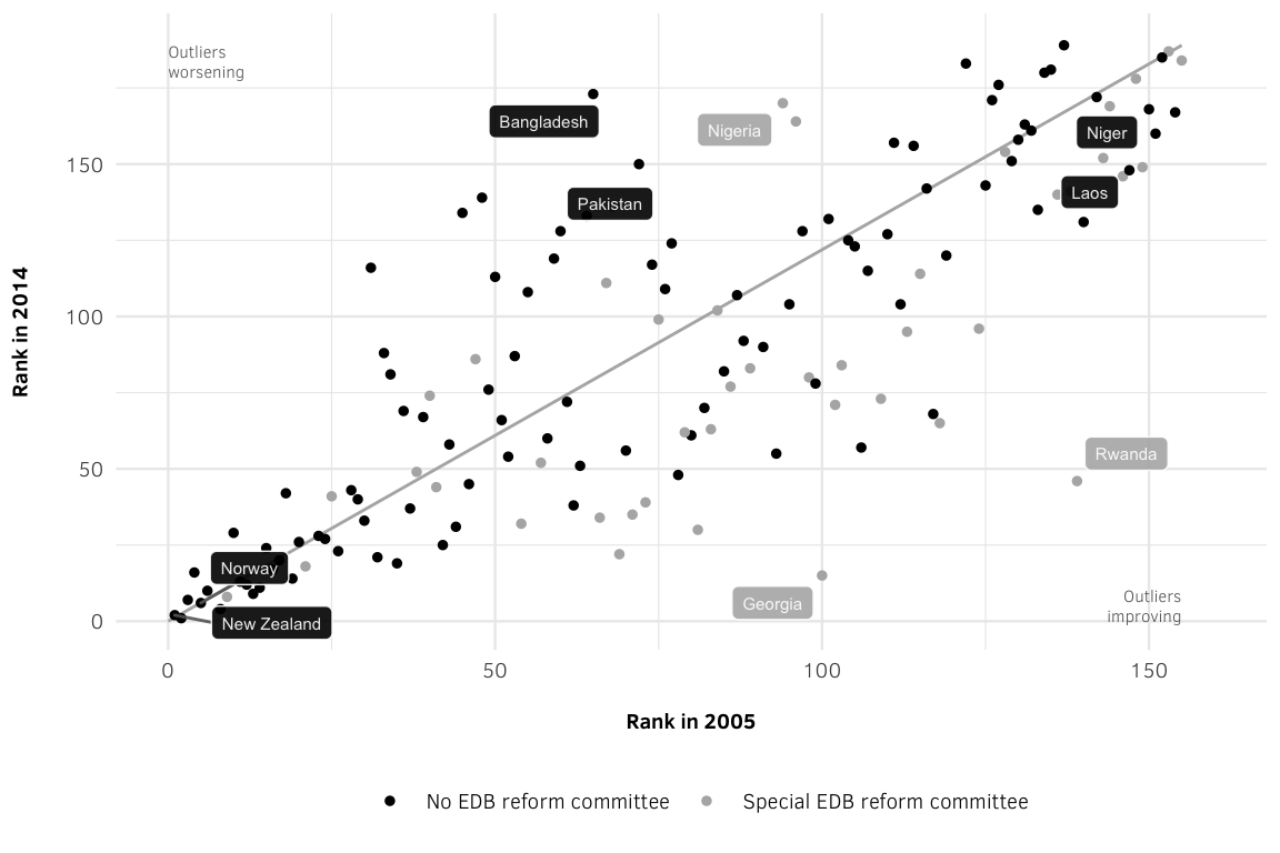
set.seed(1234)
ggsave(fig_rankings_corr,
       filename = file.path(here(), "output", "figures", "bureau_rankings.pdf"),
       width = 6, height = 4, units = "in", device = cairo_pdf)
set.seed(1234)
ggsave(fig_rankings_corr,
       filename = file.path(here(), "output", "figures", "bureau_rankings.png"),
       width = 6, height = 4, units = "in", type = "cairo", dpi = 300)
Figure 4: Ranking Gains by Number of Reforms, by Committee Status (95% CI)
Every reform leads to a negative change in rankings (which is good) in the following year for countries with special EDB reform committees. For instance, doing an enforcing contracts reform will move a country down (i.e. to a better position) nearly 6 positions. This is also the case when normalizing rankings to a 0-100 scale to account for the changing number of rank positions over time.
# Add new columns for leaded rankings and changes in rankings
change_in_rankings_norm <- edb_clean %>%
  select(ccode, country_name, year, p_edb_rank, p_edb_rank_normalized, has_bureau) %>%
  mutate(rank0 = p_edb_rank,
         rank1 = lead(rank0, 1),
         rank2 = lead(rank0, 2),
         change1 = rank1 - rank0,
         change2 = rank2 - rank0,
         rank0_norm = p_edb_rank_normalized,
         rank1_norm = lead(rank0_norm, 1),
         rank2_norm = lead(rank0_norm, 2),
         change1_norm = rank1_norm - rank0_norm,
         change2_norm = rank2_norm - rank0_norm) %>%
  filter(year >= 2005)

# Calculate the changes--or bumps--in rankings per reform undertaken
edb_reforms_rankings_bumps <- edb_reforms %>%
  filter(!str_detect(reform_type, "lag")) %>%
  group_by(ccode, year, reform_type_clean) %>%
  summarise(num_reforms = sum(reform_num_no_na)) %>%
  left_join(change_in_rankings_norm, by = c("ccode", "year")) %>%
  filter(num_reforms != 0) %>%
  mutate(change_per_reform1 = change1 / num_reforms,
         change_per_reform2 = change2 / num_reforms,
         change_per_reform1_norm = change1_norm / num_reforms,
         change_per_reform2_norm = change2_norm / num_reforms)

# Calculate summary statistics of bumps in rankings
edb_reforms_rankings_bumps_summarized <- edb_reforms_rankings_bumps %>%
  group_by(reform_type_clean, has_bureau) %>%
  summarise(avg_bump_norm = mean(change_per_reform1_norm, na.rm = TRUE),
            stderr_bump_norm = sd(change_per_reform1_norm, na.rm = TRUE) /
              sqrt(length(change_per_reform1_norm)),
            lower_norm = avg_bump_norm + (qnorm(0.025) * stderr_bump_norm),
            upper_norm = avg_bump_norm + (qnorm(0.975) * stderr_bump_norm),
            avg_bump = mean(change_per_reform1, na.rm = TRUE),
            stderr_bump = sd(change_per_reform1, na.rm = TRUE) /
              sqrt(length(change_per_reform1)),
            lower = avg_bump + (qnorm(0.025) * stderr_bump),
            upper = avg_bump + (qnorm(0.975) * stderr_bump)) %>%
  ungroup() %>%
  arrange(desc(has_bureau), desc(avg_bump)) %>%
  filter(!is.na(reform_type_clean)) %>%
  mutate(reform_type_clean = factor(reform_type_clean,
                                    levels = unique(reform_type_clean),
                                    ordered = TRUE))
plot_ranking_bumps_norm <- ggplot(edb_reforms_rankings_bumps_summarized,
aes(x = avg_bump_norm, y = reform_type_clean, colour = has_bureau)) +
geom_vline(xintercept = 0, colour = "black", size = 0.5) +
geom_pointrangeh(aes(xmin = lower_norm, xmax = upper_norm), size = 0.5,
position = position_dodgev(0.5)) +
scale_color_manual(values = c(color_no_committee, color_committee), name = NULL) +
labs(x = "Average change in EDB rankings one year after reform (normalized rankings)",
y = "Type of reform") +
theme_edb()
plot_ranking_bumps_norm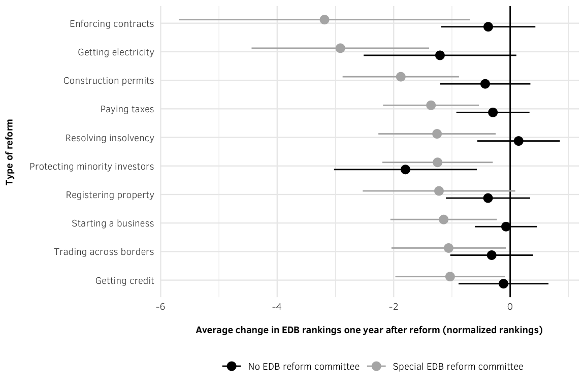
ggsave(plot_ranking_bumps_norm,
       filename = file.path(here(), "output", "figures", "bureau_rankings_bumps.pdf"),
       width = 6, height = 4, units = "in", device = cairo_pdf)
ggsave(plot_ranking_bumps_norm,
       filename = file.path(here(), "output", "figures", "bureau_rankings_bumps.png"),
width = 6, height = 4, units = "in", type = "cairo", dpi = 300)t-tests for changes in rankings
edb_reforms_rankings_bumps_tests <- edb_reforms_rankings_bumps %>%
  ungroup() %>%
  select(has_bureau, reform_type_clean, change_per_reform1_norm) %>%
  gather(variable, value, -has_bureau, -reform_type_clean) %>%
  group_by(reform_type_clean, has_bureau) %>%
  summarise(data = list(value)) %>%
  spread(has_bureau, data) %>%
  mutate(t_test = list(t.test(unlist(`No EDB reform committee`),
                              unlist(`Special EDB reform committee`))),
         t_value = t_test %>% map_dbl("statistic"),
         p_value = t_test %>% map_dbl("p.value"),
         estimate = t_test %>% map("estimate"),
         mean_committee = estimate %>% map_dbl(~ .x[2]),
         mean_no_committee = estimate %>% map_dbl(~ .x[1]),
         diff_in_means = estimate %>% map_dbl(~ abs(.x[2] - .x[1]))) %>%
  mutate(t = paste0(sprintf("%.2f", round(t_value, 2)), p_stars(p_value))) %>%
  arrange(mean_committee) %>%
  select(Reform = reform_type_clean,
         `Average change in rankings, committee` = mean_committee,
         `Average change in rankings, no committee` = mean_no_committee,
         `Difference in means` = diff_in_means, `*t*` = t)

caption <- 'Differences in average change in EDB rankings by reform, by committee status'

tbl_edb_reforms_diffs <- pandoc.table.return(edb_reforms_rankings_bumps_tests,
                                             caption = caption, split.tables = Inf,
                                             digits = 2, justify = "lcccc")

cat(tbl_edb_reforms_diffs)| Reform | Average change in rankings, committee | Average change in rankings, no committee | Difference in means | t |
|---|---|---|---|---|
| Enforcing contracts | -3.2 | -0.38 | 2.8 | 2.01* |
| Getting electricity | -2.9 | -1.2 | 1.7 | 1.47 |
| Construction permits | -1.9 | -0.43 | 1.4 | 2.10** |
| Paying taxes | -1.4 | -0.3 | 1.1 | 1.88* |
| Resolving insolvency | -1.3 | 0.14 | 1.4 | 2.15** |
| Protecting minority investors | -1.2 | -1.8 | 0.55 | -0.58 |
| Registering property | -1.2 | -0.38 | 0.84 | 1.03 |
| Starting a business | -1.1 | -0.072 | 1.1 | 1.86* |
| Trading across borders | -1.1 | -0.32 | 0.74 | 1.11 |
| Getting credit | -1 | -0.11 | 0.92 | 1.36 |
cat(tbl_edb_reforms_diffs,
    file = file.path(here(), "output", "tables", "table_edb_reforms_diffs.md"))
*p<0.1; **p<0.05; ***p<0.01
Figure 5: Public Assessments of Importance of Improving India’s Business Climate and EDB Rankings, by Exposure to EDB Information
chn_ind_assessments <- read_csv(file.path(here(), "data_raw", "chn-ind-assessments.csv")) %>%
  rename(Frame = X1) %>%
  gather(key, value, -Frame)

# Split into two data frames for faceting, then recombine
chn_ind_both <- chn_ind_assessments %>%
  filter(key %in% c("India Higher", "No Rank", "China Higher")) %>%
  mutate(comparison = "Both")

ind_only <- chn_ind_assessments %>%
  filter(key %in% c("No Rank", "India's Rank Only")) %>%
  mutate(comparison = "India only")

blank_country <- data_frame(Frame = unique(chn_ind_assessments$Frame),
                            key = " ", value = c(0, 0),
                            comparison = "India only")

chn_ind_plot_data <- bind_rows(chn_ind_both, ind_only, blank_country) %>%
  mutate(key = factor(key, levels = c("India Higher", "India's Rank Only",
                                      "No Rank", "China Higher", " "),
                      ordered = TRUE),
         Frame = fct_inorder(Frame, ordered = TRUE))

chn_ind_annotations <- data_frame(x = c(4, 5), y = c(0.6, 0.6),
                                  text = c("Lower importance", "Higher importance"),
                                  hjust = c("left", "right"))

# Plot
plot_chn_ind <- ggplot(chn_ind_plot_data, aes(x = value, y = fct_rev(key),
                                              color = fct_rev(Frame))) +
  geom_pointrangeh(aes(xmin = 0, xmax = value), size = 0.5,
                   position = position_dodgev(height = 0.5)) +
  geom_text(data = chn_ind_annotations,
            aes(x = x, y = y, label = text, hjust = hjust),
            vjust = "center", color = "grey40", size = 2, lineheight = 1) +
  geom_text(aes(label = value), position = position_dodgev(height = 0.5),
            hjust = -0.4, size = 2.5) +
  scale_color_manual(values = c(edb_importance, climate_importance), name = NULL,
                     guide = guide_legend(reverse = TRUE)) +
  scale_x_continuous(breaks = seq(0, 5, 0.5)) +
  coord_cartesian(xlim = c(4, 5)) +
  labs(x = NULL, y = NULL) +
  theme_edb() +
  theme(strip.text = element_blank(),
        panel.grid.minor = element_blank(),
        panel.grid.major.y = element_blank()) +
  facet_wrap(~ comparison, scales = "free_y")

plot_chn_ind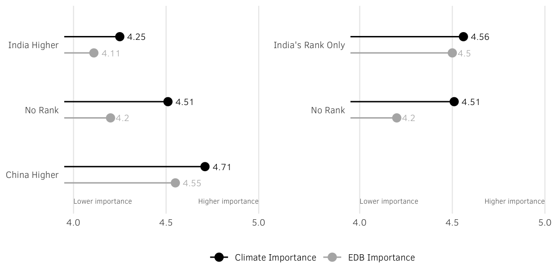
ggsave(plot_chn_ind,
       filename = file.path(here(), "output", "figures", "chn_ind_exposure.pdf"),
       width = 6, height = 3, units = "in", device = cairo_pdf)
ggsave(plot_chn_ind,
       filename = file.path(here(), "output", "figures", "chn_ind_exposure.png"),
       width = 6, height = 3, units = "in", type = "cairo", dpi = 300)