Difference-in-differences

library(tidyverse)
library(targets)
library(modelsummary)
library(tinytable)
library(scales)
library(ggdag)
library(dagitty)
library(parameters)

tar_config_set(
  store = here::here('_targets'),
  script = here::here('_targets.R')
)

did <- tar_read(data_did)

invisible(list2env(tar_read(graphic_functions), .GlobalEnv))
set_annotation_fonts()

gof_map <- tribble(
  ~raw,            ~clean,               ~fmt, ~omit,
  "nobs",          "N",                  0,    FALSE,
  "r.squared",     "$R^2$",          2,    FALSE,
  "adj.r.squared", "\\(R^2\\) adjusted", 2,    FALSE
)

Parallel trends

did |> 
  group_by(school, year) |> 
  summarize(mean = ggplot2::mean_se(prosocial_index, mult = 1.96)) |> 
  unnest(mean) |> 
  ggplot(aes(x = year, y = y, color = school)) +
  geom_vline(xintercept = 2022.5, linetype = "dashed") +
  geom_line(linewidth = 0.25, show.legend = FALSE) +
  geom_pointrange(aes(ymin = ymin, ymax = ymax)) +
  scale_color_manual(values = c(clrs$Prism[2], clrs$Prism[8])) +
  labs(x = NULL, y = "Prosocial index", color = NULL) +
  theme_np(base_size = 16)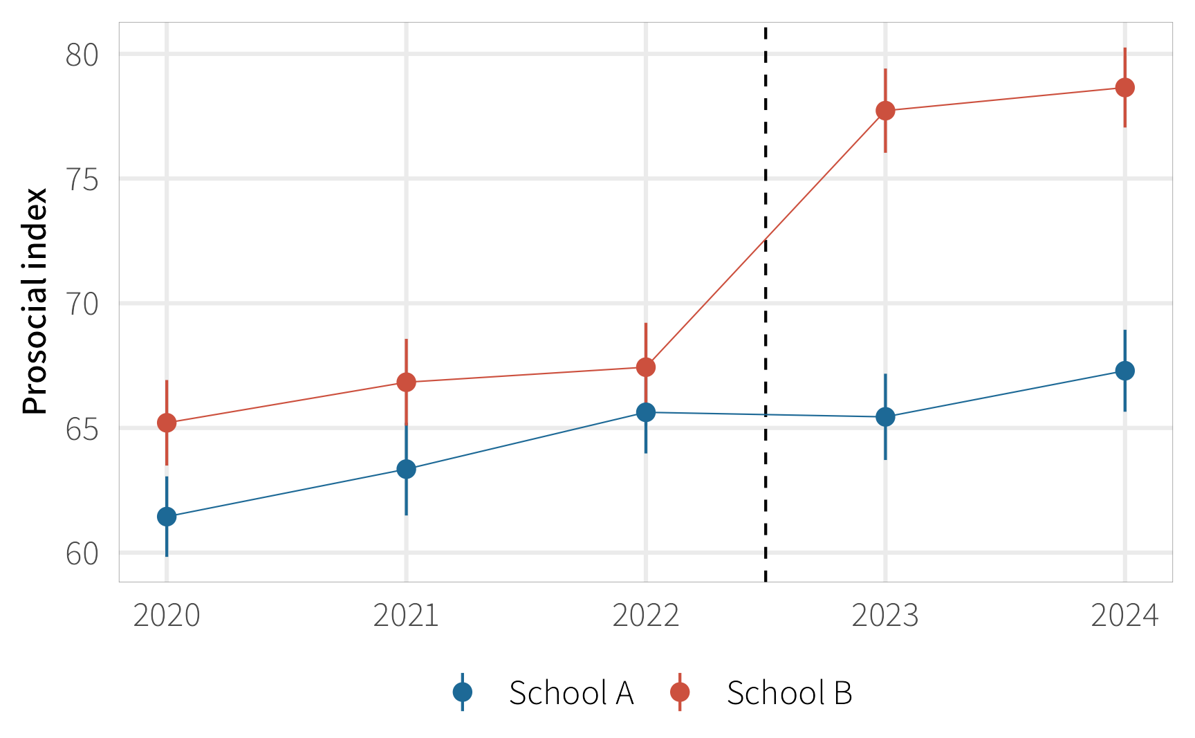

Models

model_small <- lm(
  prosocial_index ~ school + factor(year) + school*factor(year),
  data = filter(did, year %in% c(2022, 2023))
)

model_small_controls <- lm(
  prosocial_index ~ school + factor(year) + school*factor(year) +
    social_awareness + age + gpa + income,
  data = filter(did, year %in% c(2022, 2023))
)

model_full <- lm(
  prosocial_index ~ school + factor(year) + I(school == "School B" & year >= 2023),
  data = did
)

model_full_controls <- lm(
  prosocial_index ~ school + factor(year) + I(school == "School B" & year >= 2023) +
    social_awareness + age + gpa + income,
  data = did
)

models <- list(
  "Interaction term only" = model_small,
  "Interaction term + covariates" = model_small_controls,
  "Interaction term only (all years)" = model_full,
  "Interaction term + covariates (all years)" = model_full_controls
)

modelsummary(
  models,
  statistic = "[{conf.low}, {conf.high}]",
  fmt = 2,
  gof_map = gof_map,
  add_columns = tibble("True effect" = c(NA, NA, 10)) |> magrittr::set_attr("position", 2)
)# |>

	True effect	Interaction term only	Interaction term + covariates	Interaction term only (all years)	Interaction term + covariates (all years)
(Intercept)		65.63	-4.00	61.82	-7.44
		[63.91, 67.34]	[-11.07, 3.07]	[60.42, 63.21]	[-12.08, -2.80]
schoolSchool B	10.00	1.81	1.73	3.02	2.14
		[-0.62, 4.24]	[0.21, 3.24]	[1.63, 4.41]	[1.27, 3.01]
factor(year)2023		-0.18	1.09	3.86	4.47
		[-2.61, 2.25]	[-0.44, 2.61]	[1.83, 5.89]	[3.21, 5.74]
schoolSchool B × factor(year)2023		10.47	8.30
		[7.04, 13.90]	[6.14, 10.45]
social_awareness			0.47		0.47
			[0.43, 0.51]		[0.44, 0.49]
age			0.69		0.64
			[0.47, 0.91]		[0.50, 0.78]
gpa			3.29		3.82
			[2.33, 4.25]		[3.18, 4.45]
income			0.00		0.00
			[0.00, 0.00]		[0.00, 0.00]
factor(year)2021				1.77	1.71
				[0.06, 3.47]	[0.65, 2.77]
factor(year)2022				3.21	3.15
				[1.50, 4.91]	[2.08, 4.21]
factor(year)2024				5.25	6.16
				[3.22, 7.28]	[4.89, 7.43]
I(school == "School B" & year >= 2023)TRUE				8.80	7.76
				[6.60, 11.00]	[6.39, 9.14]
N		504	504	1260	1260
$R^2$		0.21	0.70	0.24	0.70
$R^2$ adjusted		0.21	0.70	0.23	0.70

  # style_tt(
  #   i = 3:4, j = 1:6, 
  #   background = clrs$Prism[6], color = "#ffffff", bold = TRUE
  # )

modelsummary(
  models,
  statistic = "[{conf.low}, {conf.high}]",
  fmt = 2,
  coef_map = c(
    `schoolSchool B:factor(year)2023` = "School B × 2023",
    `I(school == "School B" & year >= 2023)TRUE` = "School B × 2023"
  ),
  gof_map = gof_map,
  add_columns = tibble("True effect" = 10) |> magrittr::set_attr("position", 2)
)

	True effect	Interaction term only	Interaction term + covariates	Interaction term only (all years)	Interaction term + covariates (all years)
School B × 2023	10.00	10.47	8.30	8.80	7.76
		[7.04, 13.90]	[6.14, 10.45]	[6.60, 11.00]	[6.39, 9.14]
N		504	504	1260	1260
$R^2$		0.21	0.70	0.24	0.70
$R^2$ adjusted		0.21	0.70	0.23	0.70

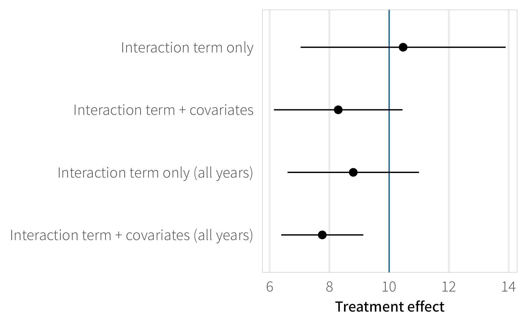
treatment_effects <- enframe(models) |> 
  mutate(params = map(value, \(x) model_parameters(x))) |> 
  unnest(params) |> 
  filter(Parameter %in% c("schoolSchool B:factor(year)2023", 'I(school == "School B" & year >= 2023)TRUE')) |> 
  mutate(name = factor(name, levels = names(models)))

ggplot(treatment_effects, aes(x = Coefficient, y = fct_rev(name))) +
  geom_vline(xintercept = 10, color = clrs$Prism[2]) +
  geom_pointrange(aes(xmin = CI_low, xmax = CI_high)) +
  labs(x = "Treatment effect", y = NULL) +
  theme_np(base_size = 16) +
  theme(panel.grid.major.y = element_blank())