Post draft

library(tidyverse)        # ggplot, dplyr, and friends
library(haven)            # Read Stata files
library(broom)            # Convert model objects to tidy data frames
library(parameters)
# library(cregg)            # Automatically calculate frequentist conjoint AMCEs and MMs
library(survey)           # Panel-ish regression models
library(mlogit)
library(dfidx)
library(scales)           # Nicer labeling functions
library(marginaleffects)  # Calculate marginal effects
# library(broom.helpers)    # Add empty reference categories to tidy model data frames
library(ggforce)          # For facet_col()
library(brms)             # The best formula-based interface to Stan
library(tidybayes)        # Manipulate Stan results in tidy ways
library(ggdist)           # Fancy distribution plots
library(patchwork)        # Combine ggplot plots
library(glue)

# Custom ggplot theme to make pretty plots
# Get the font at https://github.com/intel/clear-sans
theme_nice <- function() {
  theme_minimal(base_family = "Clear Sans") +
    theme(panel.grid.minor = element_blank(),
          plot.title = element_text(family = "Clear Sans", face = "bold"),
          axis.title.x = element_text(hjust = 0),
          axis.title.y = element_text(hjust = 1),
          strip.text = element_text(family = "Clear Sans", face = "bold",
                                    size = rel(0.75), hjust = 0),
          strip.background = element_rect(fill = "grey90", color = NA))
}

# Set default theme and font stuff
theme_set(theme_nice())
update_geom_defaults("text", list(family = "Clear Sans", fontface = "plain"))
update_geom_defaults("label", list(family = "Clear Sans", fontface = "plain"))


# Functions for formatting things as percentage points
label_pp <- label_number(accuracy = 1, scale = 100, 
                         suffix = " pp.", style_negative = "minus")

label_amce <- label_number(accuracy = 0.1, scale = 100, suffix = " pp.", 
                           style_negative = "minus", style_positive = "plus")

chocolate_simple <- read_csv("data/choco_candy.csv") %>% 
  mutate(
    dark = case_match(dark, 0 ~ "Milk", 1 ~ "Dark"),
    dark = factor(dark, levels = c("Milk", "Dark")),
    soft = case_match(soft, 0 ~ "Chewy", 1 ~ "Soft"),
    soft = factor(soft, levels = c("Chewy", "Soft")),
    nuts = case_match(nuts, 0 ~ "No nuts", 1 ~ "Nuts"),
    nuts = factor(nuts, levels = c("No nuts", "Nuts"))
  )

I was always under the impression that multinomial logit means that the outcome variable is an unordered categorical variable with more than 2 categories (while regular logit is for binary categorical outcomes and ordered logit is for 2+ categories that have an inherent order), but apparently this counts? idk

Example 1: Basic multinomial logit with chocolate candy

The setup

Example survey question

Respondents only see this question one time—all possible options are presented simultaneously.

	A	B	C	D	E	F	G	H
Chocolate	Milk	Milk	Milk	Milk	Dark	Dark	Dark	Dark
Center	Chewy	Chewy	Soft	Soft	Chewy	Chewy	Soft	Soft
Nuts	No nuts	Nuts	No nuts	Nuts	No nuts	Nuts	No nuts	Nuts
Choice

The data

The data for this kind of experiment looks like this, with one row for each possible alternative (so eight rows per person, or subj), with the alternative that was selected marked as 1 in choice. Here, Subject 1 chose option E (dark, chewy, no nuts).

chocolate_simple
## # A tibble: 80 × 6
##     subj choice alt   dark  soft  nuts   
##    <dbl>  <dbl> <chr> <fct> <fct> <fct>  
##  1     1      0 A     Milk  Chewy No nuts
##  2     1      0 B     Milk  Chewy Nuts   
##  3     1      0 C     Milk  Soft  No nuts
##  4     1      0 D     Milk  Soft  Nuts   
##  5     1      1 E     Dark  Chewy No nuts
##  6     1      0 F     Dark  Chewy Nuts   
##  7     1      0 G     Dark  Soft  No nuts
##  8     1      0 H     Dark  Soft  Nuts   
##  9     2      0 A     Milk  Chewy No nuts
## 10     2      0 B     Milk  Chewy Nuts   
## # ℹ 70 more rows

The model

Original SAS model as a baseline

lol SAS

I know nothing about SAS. I have never opened SAS in my life. It is a mystery to me.

I copied these results directly from p. 297 in the massive “Discrete Choice” technical note by Warren. F. Kuhfeld.

I only have this SAS output here as a baseline reference for what the actual correct coefficients are supposed to be.

SAS apparently fits these models with proportional hazard survival-style models, which feels weird, but there’s probably a mathematical or statistical reason for it. You use PROC PHREG to do it:

proc phreg data=chocs outest=betas;
   strata subj set;
   model c*c(2) = dark soft nuts / ties=breslow;
   run;

It gives these results:

                   Choice of Chocolate Candies

                       The PHREG Procedure

              Multinomial Logit Parameter Estimates
              
                      Parameter     Standard
                 DF    Estimate        Error  Chi-Square   Pr > ChiSq
Dark Chocolate   1      1.38629      0.79057      3.0749       0.0795
Soft Center      1     -2.19722      1.05409      4.3450       0.0371
With Nuts        1      0.84730      0.69007      1.5076       0.2195

Survival model

Ew, enough SAS. Let’s do this with R instead.

We can recreate the same proportional hazards model with coxph() from the {survival} package. Again, this feels weird and not like an intended purpose of survival models and not like multinomial logit at all—in my mind it is neither (1) multinomial nor (2) logit, but whatever. People far smarter than me invented these things, so I’ll just trust them.

model_basic_survival <- coxph(
  Surv(subj, choice) ~ dark + soft + nuts, 
  data = chocolate_simple, 
  ties = "breslow"  # This is what SAS uses
)

model_parameters(model_basic_survival, digits = 4, p_digits = 4)
## Parameter   | Coefficient |     SE |         95% CI |       z |      p
## ----------------------------------------------------------------------
## dark [Dark] |      1.3863 | 0.7906 | [-0.16,  2.94] |  1.7535 | 0.0795
## soft [Soft] |     -2.1972 | 1.0541 | [-4.26, -0.13] | -2.0845 | 0.0371
## nuts [Nuts] |      0.8473 | 0.6901 | [-0.51,  2.20] |  1.2279 | 0.2195

The coefficients, standard errors, and p-values are identical to the SAS output! The only difference is the statistic: in SAS they use a chi-square statistic, while survival:coxph() uses a z statistic. There’s probably a way to make coxph() use a chi-square statistic, but I don’t care about that. I never use survival models and I’m only doing this to replicate the SAS output and it just doesn’t matter.

Poisson model

An alternative way to fit a multinomial logit model without resorting to survival models is to actually (mis?)use another model family. We can use a Poisson model, even though choice isn’t technically count data, because of obscure stats reasons.¹ To account for the repeated subjects in the data, we’ll use svyglm() from the {survey} package so that the standard errors are more accurate.

model_basic_poisson <- glm(
  choice ~ dark + soft + nuts, 
  data = chocolate_simple, 
  family = poisson()
)

model_parameters(model_basic_poisson, digits = 4, p_digits = 4)
## Parameter   | Log-Mean |     SE |         95% CI |       z |      p
## -------------------------------------------------------------------
## (Intercept) |  -2.9188 | 0.8628 | [-4.97, -1.49] | -3.3829 | 0.0007
## dark [Dark] |   1.3863 | 0.7906 | [ 0.00,  3.28] |  1.7535 | 0.0795
## soft [Soft] |  -2.1972 | 1.0541 | [-5.11, -0.53] | -2.0845 | 0.0371
## nuts [Nuts] |   0.8473 | 0.6901 | [-0.43,  2.38] |  1.2279 | 0.2195

Lovely—the results are the same.

`mlogit` model

Finally, we can use the {mlogit} package to fit the model. Before using mlogit(), we need to transform our data a bit to specify which column represents the choice (choice) and how the data is indexed (subjects (subj) with repeated alternatives (alt)

chocolate_simple_idx <- dfidx(
  chocolate_simple,
  idx = list("subj", "alt"),
  choice = "choice",
  shape = "long"
)

We can then use this indexed dataframe with mlogit(), which uses the familiar R forumla interface, but with some extra features separated by |s

outcome ~ features | individual-level variables | alternative-level variables

If we had columns related to individual-level characteristics or alternative-level characteristics, we could include those in the model—and we’ll do precisely that later in this post. (Incorporating individual-level covariates is the whole point of this post!)

Let’s fit the model:

model_basic_mlogit <- mlogit(
  choice ~ dark + soft + nuts | 0 | 0, 
  data = chocolate_simple_idx
)

model_parameters(model_basic_mlogit, digits = 4, p_digits = 4)
## Parameter   | Log-Odds |     SE |         95% CI |       z |      p
## -------------------------------------------------------------------
## dark [Dark] |   1.3863 | 0.7906 | [-0.16,  2.94] |  1.7535 | 0.0795
## soft [Soft] |  -2.1972 | 1.0541 | [-4.26, -0.13] | -2.0845 | 0.0371
## nuts [Nuts] |   0.8473 | 0.6901 | [-0.51,  2.20] |  1.2279 | 0.2195

Delightful. All the results are the same as the survival model and the Poisson model, but this feels less hacky than the other two approaches.

Bayesian model

We can also fit this model in a Bayesian way using {brms}. Stan has a categorical distribution family for multinomial models, but it’s designed for outcomes that are mulitnomial in the sense of having multiple unordered categories, not this 0/1 weirdness we’re using here. So instead, we’ll use a Poisson family, since, as we saw above, that’s a legal way of parameterizing multinomial distributions.

The data has a natural hierarchical structure to it, with 8 choices (for alternatives A through H) nested inside each subject.

Multilevel experimental structure, with candy choices $y_{\text{A}\dots\text{H}}$ nested in subjects

We want to model candy choice (choice) based on candy characteristics (dark, soft, and nuts). We’ll use the subscript $i$ to refer to individual candy choices and $j$ to refer to subjects.

Since we can legally pretend that this multinomial selection process is actually Poisson, we’ll model it as a Poisson process that has a rate of $\lambda_{i_j}$. We’ll model that $\lambda_{i_j}$ with a log-linked regression model with covariates for each of the levels of each candy feature. To account for the multilevel structure, we’ll include subject-specific offsets ($b_{0_j}$) from the global average, thus creating random intercepts. We’ll specify fairly wide priors just because.

Here’s the formal model for all this:

\[ \begin{aligned} \text{Choice}_{i_j} \sim&\ \operatorname{Poisson}(\lambda_{i_j}) & \text{Probability of selection for choice}_i \text{ in subject}_j \\ \log(\lambda_{i_j}) =&\ (\beta_0 + b_{0_j}) + \beta_1 \text{Dark}_{i_j} + & \text{Model for probability}\\ &\ \beta_2 \text{Soft}_{i_j} + \beta_3 \text{Nuts}_{i_j} \\ b_{0_j} \sim&\ \mathcal{N}(0, \sigma_0) & \text{Subject-specific offsets from global choice probability} \\ \\ \beta_0 \sim&\ \mathcal{N}(0, 3) & \text{Prior for global average choice probability} \\ \beta_1, \beta_2, \beta_3 \sim&\ \mathcal{N}(0, 3) & \text{Prior for candy feature levels} \\ \sigma_0 \sim&\ \operatorname{Exponential}(1) & \text{Prior for between-subject variability} \end{aligned} \]

And here’s the {brms} model:

model_basic_brms <- brm(
  bf(choice ~ dark + soft + nuts + (1 | subj)),
  data = chocolate_simple,
  family = poisson(),
  prior = c(
    prior(normal(0, 3), class = Intercept),
    prior(normal(0, 3), class = b),
    prior(exponential(1), class = sd)
  ),
  chains = 4, cores = 4, iter = 2000, seed = 1234,
  backend = "cmdstanr", threads = threading(2), refresh = 0,
  file = "model_basic_brms"
)

The results are roughly the same as what we found with all the other models—they’re slightly off because of random MCMC sampling.

model_parameters(model_basic_brms)
## # Fixed Effects
## 
## Parameter   | Median |         95% CI |     pd |  Rhat |     ESS
## ----------------------------------------------------------------
## (Intercept) |  -3.04 | [-5.07, -1.60] |   100% | 1.000 | 3598.00
## darkDark    |   1.35 | [-0.05,  3.16] | 96.92% | 1.000 | 4238.00
## softSoft    |  -2.03 | [-4.35, -0.47] | 99.60% | 1.000 | 2867.00
## nutsNuts    |   0.83 | [-0.40,  2.27] | 90.28% | 1.000 | 4648.00

Predictions

In the SAS technical note example, they use the model to generated predicted probabilities of the choice of each of the options. In the world of marketing, this can also be seen as the predicted market share for each option. To do this, they plug each of the eight different different combinations of dark, soft, and nuts into the model and calculate the predicted output on the response (i.e. probability) scale. They get these results, where dark, chewy, and nuts is the most likely and popular option (commanding a 50% market share).

      Choice of Chocolate Candies

Obs    Dark    Soft     Nuts       p

  1    Dark    Chewy    Nuts       0.50400
  2    Dark    Chewy    No Nuts    0.21600
  3    Milk    Chewy    Nuts       0.12600
  4    Dark    Soft     Nuts       0.05600
  5    Milk    Chewy    No Nuts    0.05400
  6    Dark    Soft     No Nuts    0.02400
  7    Milk    Soft     Nuts       0.01400
  8    Milk    Soft     No Nuts    0.00600

We can do the same thing with R.

Frequentist predictions

{mlogit} model objects have predicted values stored in one of their slots (model_basic_mlogit$probabilities), but they’re in a weird non-tidy matrix form and I like working with tidy data. I’m also a huge fan of the {marginaleffects} package, which provides a consistent way to calculate predictions, comparisons, and slopes/marginal effects (with predictions(), comparisons(), and slopes()) for dozens of kinds of models, including mlogit() models.

So instead of wrangling the built-in mlogit() probabilities, we’ll generate predictions by feeding the model the unique combinations of dark, soft, and nuts to marginaleffects::predictions(), which will provide us with probability- or proportion-scale predictions:

preds_basic_mlogit <- predictions(
  model_basic_mlogit, 
  newdata = datagrid(dark = unique, soft = unique, nuts = unique)
)

preds_basic_mlogit %>% 
  # predictions() hides a bunch of columns; forcing it to be a tibble unhides them
  as_tibble() %>% 
  arrange(desc(estimate)) %>% 
  select(group, dark, soft, nuts, estimate, std.error, statistic, p.value)
## # A tibble: 8 × 8
##   group dark  soft  nuts    estimate std.error statistic  p.value
##   <chr> <fct> <fct> <fct>      <dbl>     <dbl>     <dbl>    <dbl>
## 1 F     Dark  Chewy Nuts     0.504     0.142       3.56  0.000373
## 2 E     Dark  Chewy No nuts  0.216     0.112       1.93  0.0540  
## 3 B     Milk  Chewy Nuts     0.126     0.0849      1.48  0.138   
## 4 H     Dark  Soft  Nuts     0.0560    0.0551      1.02  0.309   
## 5 A     Milk  Chewy No nuts  0.0540    0.0433      1.25  0.213   
## 6 G     Dark  Soft  No nuts  0.0240    0.0258      0.929 0.353   
## 7 D     Milk  Soft  Nuts     0.0140    0.0162      0.863 0.388   
## 8 C     Milk  Soft  No nuts  0.00600   0.00743     0.808 0.419

Perfect! They’re identical to the SAS output.

We can play around with these predictions to describe the overall market for candy. Chewy candies dominate the market…

preds_basic_mlogit %>% 
  group_by(dark) %>% 
  summarize(share = sum(estimate))
## # A tibble: 2 × 2
##   dark  share
##   <fct> <dbl>
## 1 Milk  0.200
## 2 Dark  0.800

…and dark chewy candies are by far the most popular:

preds_basic_mlogit %>% 
  group_by(dark, soft) %>% 
  summarize(share = sum(estimate))
## # A tibble: 4 × 3
## # Groups:   dark [2]
##   dark  soft   share
##   <fct> <fct>  <dbl>
## 1 Milk  Chewy 0.180 
## 2 Milk  Soft  0.0200
## 3 Dark  Chewy 0.720 
## 4 Dark  Soft  0.0800

Bayesian predictions

{marginaleffects} supports {brms} models too, so we can basically run the same predictions() function to generate predictions for our Bayesian model. Magical.

lol subject offsets

When plugging values into predictions() (or avg_slopes() or any function that calculates predictions from a model), we have to decide how to handle the random subject offsets ($b_{0_j}$). I have a whole other blog post guide about this and how absolutely maddening the nomenclature for all this is.

By default, predictions() and friends will calculate predictions for subjects on average by using the re_formula = NULL argument. This estimate includes details from the random offsets, either by integrating them out or by using the mean and standard deviation of the random offsets to generate a simulated average subject. When working with slopes, this is also called a marginal effect.

We could also use re_formula = NA to calculate predictions for a typical subject, or a subject where the random offset is set to 0. When working with slopes, this is also called a conditional effect.

Conditional predictions/effect = average subject = re_formula = NA
Marginal predictions/effect = subjects on average = re_formula = NULL (default), using existing subject levels or a new simulated subject

Again, see this guide for way more about these distinctions. In this example here, we’ll just use the default marginal predictions/effects (re_formula = NULL), or the effect for subjects on average.

The predicted proportions aren’t identical to the SAS output, but they’re close enough, given that it’s a completely different modeling approach.

preds_basic_brms <- predictions(
  model_basic_brms, 
  newdata = datagrid(dark = unique, soft = unique, nuts = unique)
) 

preds_basic_brms %>% 
  as_tibble() %>%
  arrange(desc(estimate)) %>% 
  select(dark, soft, nuts, estimate, conf.low, conf.high)
## # A tibble: 8 × 6
##   dark  soft  nuts    estimate conf.low conf.high
##   <fct> <fct> <fct>      <dbl>    <dbl>     <dbl>
## 1 Dark  Chewy Nuts     0.432   0.144       1.09  
## 2 Dark  Chewy No nuts  0.186   0.0424      0.571 
## 3 Milk  Chewy Nuts     0.110   0.0168      0.419 
## 4 Dark  Soft  Nuts     0.0553  0.00519     0.279 
## 5 Milk  Chewy No nuts  0.0465  0.00552     0.219 
## 6 Dark  Soft  No nuts  0.0230  0.00182     0.141 
## 7 Milk  Soft  Nuts     0.0136  0.00104     0.0881
## 8 Milk  Soft  No nuts  0.00556 0.000326    0.0414

Plots

Since predictions() returns a tidy data frame, we can plot these predicted probabilities (or market shares or however we want to think about them) with {ggplot2}:

p1 <- preds_basic_mlogit %>% 
  arrange(estimate) %>% 
  mutate(label = str_to_sentence(glue("{dark} chocolate, {soft} interior, {nuts}"))) %>% 
  mutate(label = fct_inorder(label)) %>% 
  ggplot(aes(x = estimate, y = label)) +
  geom_pointrange(aes(xmin = conf.low, xmax = conf.high), color = "#CC503E") +
  scale_x_continuous(labels = label_percent()) +
  labs(
    x = "Predicted probability of selection", y = NULL,
    title = "Frequentist {mlogit} predictions") +
  theme(panel.grid.minor = element_blank(), panel.grid.major.y = element_blank())

p2 <- preds_basic_brms %>% 
  posterior_draws() %>%  # Extract the posterior draws of the predictions
  arrange(estimate) %>% 
  mutate(label = str_to_sentence(glue("{dark} chocolate, {soft} interior, {nuts}"))) %>% 
  mutate(label = fct_inorder(label)) %>% 
  ggplot(aes(x = draw, y = label)) +
  stat_halfeye(normalize = "xy", fill = "#CC503E")  +
  scale_x_continuous(labels = label_percent()) +
  labs(
    x = "Predicted probability of selection", y = NULL,
    title = "Bayesian {brms} predictions") +
  theme(panel.grid.minor = element_blank(), panel.grid.major.y = element_blank()) +
  # Make the x-axis match the mlogit plot
  coord_cartesian(xlim = c(-0.05, 0.78))

p1 / p2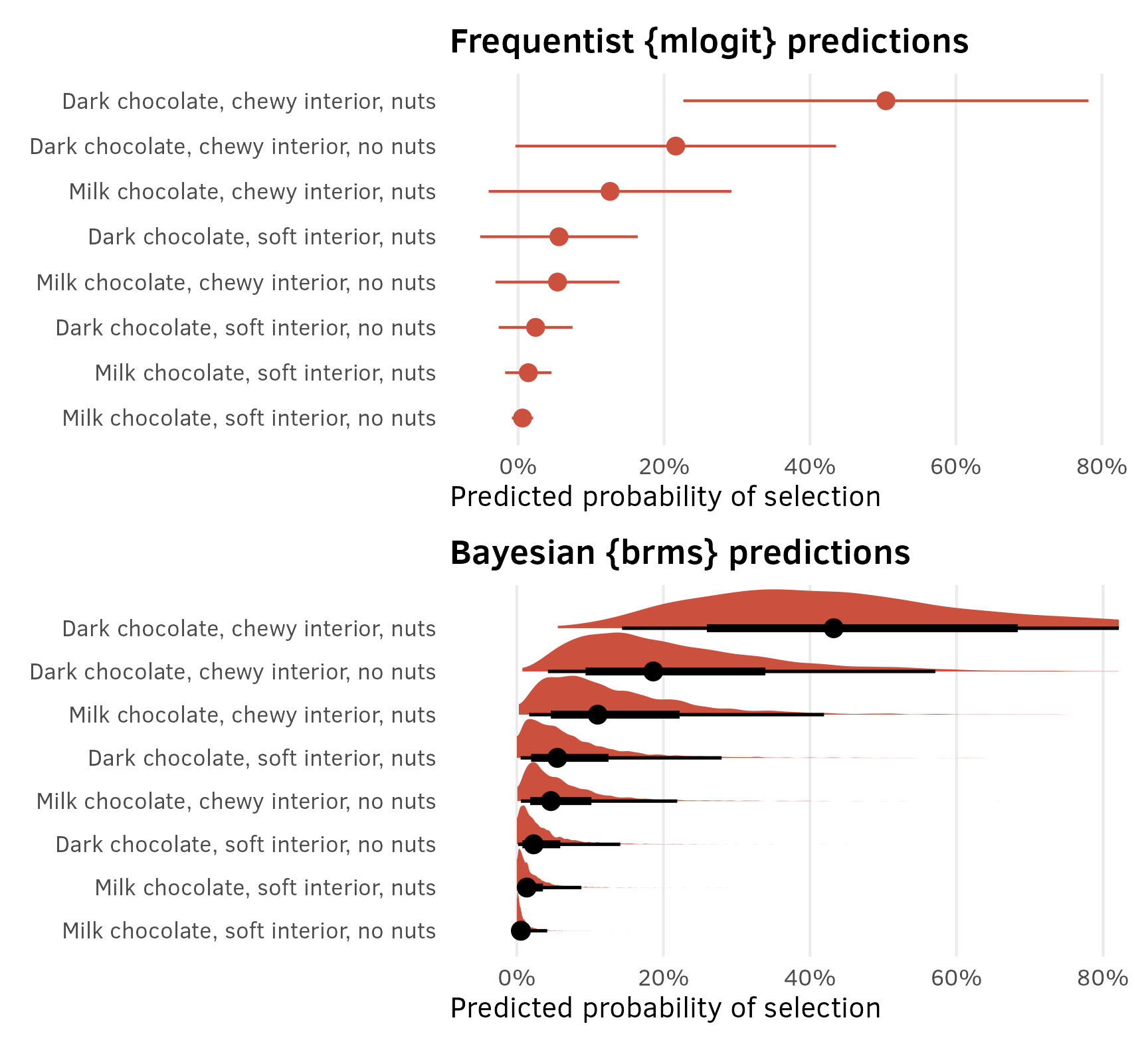

AMCEs

The marketing world doesn’t typically look at coefficients or marginal effects, but the political science world definitely does. In political science, the estimand we often care about the most is the average marginal component effect (AMCE), or the causal effect of moving one feature level to a different value, holding all other features constant. I have a whole in-depth blog post about AMCEs and how to calculate them—go look at that for more details. Long story short—AMCEs are basically the coefficients in a regression model.

Interpreting the coefficients is difficult with models that aren’t basic linear regression. Here, all these coefficients are on the log scale, so they’re not directly interpretable. The original SAS technical note also doesn’t really interpret any of these , they don’t really interpret these things anyway, since they’re more focused on predictions. All they say is this:

The parameter estimate with the smallest p-value is for soft center. Since the parameter estimate is negative, chewy is the more preferred level. Dark is preferred over milk, and nuts over no nuts, however only the p-value for Soft is less than 0.05.

We could exponentiate the coefficients to make them multiplicative (akin to odds ratios in logistic regression). For center = soft, $e^{-2.19722}$ = 0.1111, which means that candies with a soft center are 89% less likely to be chosen than candies with a chewy center, relative to the average candy. But that’s weird to think about.

So instead we can turn to {marginaleffects} once again to calculate percentage-point scale estimands that we can interpret far more easily.

lol marginal effects

Nobody is ever consistent about the word “marginal effect.” Some people use it to refer to averages; some people use it to refer to slopes. These are complete opposites. In calculus, averages = integrals and slopes = derivatives and they’re the inverse of each other.

I like to think of marginal effects as what happens to the outcome when you move an explanatory variable a tiny bit. With continuous variables, that’s a slope; with categorical variables, that’s an offset in average outcomes. These correspond directly to how you normally interpret regression coefficients. Or returning to my favorite analogy about regression, with numeric variables we care what happens to the outcome when we slide the value up a tiny bit; with categorical variables we care about what happens to the outcome when we switch on a category.

Additionally, there are like a billion different ways to calculate marginal effects: average marginal effects (AMEs), group-average marginal effects (G-AMEs), marginal effects at user-specified values, marginal effects at the mean (MEM), and counterfactual marginal effects. See the documentation for {marginaleffects} + this mega blog post for more about these subtle differences.

Bayesian comparisons/contrasts

We can use avg_comparisons() to calculate the difference (or average marginal effect) for each of the categorical coefficients on the percentage-point scale, showing the effect of moving from milk → dark, chewy → soft, and nuts → no nuts.

(Technically we can also use avg_slopes(), even though none of these coefficients are actually slopes. {marginaleffects} is smart enough to show contrasts for categorical variables and partial derivatives/slopes for continuous variables.)

avg_comparisons(model_basic_brms)
## 
##  Term       Contrast Estimate    2.5 %  97.5 %
##  dark Dark - Milk       0.139 -0.00551  0.3211
##  nuts Nuts - No nuts    0.092 -0.05221  0.2599
##  soft Soft - Chewy     -0.182 -0.35800 -0.0523
## 
## Columns: term, contrast, estimate, conf.low, conf.high

When holding all other features constant, moving from chewy → soft is associated with a posterior median 18 percentage point decrease in the probability of selection (or drop in market share if you want to think of it that way), on average

Frequentist comparisons/contrasts

We went out of order in this section and showed how to use avg_comparisons() with the Bayesian model first instead of the frequentist model. That’s because it was easy. mlogit() models behave strangely with {marginaleffects} because {mlogit} forces its predictions to use every possible value of the alternatives A–H. Accordingly, the estimate for any coefficients in the attributes section of the {mlogit} formula (dark, soft, and nuts here) will automatically be zero. Note how here there are 24 rows of comparisons instead of 3, since we get comparisons in each of the 8 groups, and note how the estimates are all zero:

avg_comparisons(model_basic_mlogit)
## 
##  Group Term       Contrast  Estimate Std. Error         z Pr(>|z|)    S     2.5 %   97.5 %
##      A dark Dark - Milk    -2.78e-17   7.27e-13 -3.82e-05        1  0.0 -1.42e-12 1.42e-12
##      B dark Dark - Milk     0.00e+00         NA        NA       NA   NA        NA       NA
##      C dark Dark - Milk     0.00e+00   1.62e-14  0.00e+00        1 -0.0 -3.17e-14 3.17e-14
##      D dark Dark - Milk    -6.94e-18   1.73e-13 -4.02e-05        1  0.0 -3.38e-13 3.38e-13
##      E dark Dark - Milk    -2.78e-17   7.27e-13 -3.82e-05        1  0.0 -1.42e-12 1.42e-12
##      F dark Dark - Milk     0.00e+00         NA        NA       NA   NA        NA       NA
##      G dark Dark - Milk     0.00e+00   1.62e-14  0.00e+00        1 -0.0 -3.17e-14 3.17e-14
##      H dark Dark - Milk    -6.94e-18   1.73e-13 -4.02e-05        1  0.0 -3.38e-13 3.38e-13
##      A soft Soft - Chewy    6.94e-18   1.08e-13  6.42e-05        1  0.0 -2.12e-13 2.12e-13
##      B soft Soft - Chewy    1.39e-17   2.16e-13  6.43e-05        1  0.0 -4.23e-13 4.23e-13
##      C soft Soft - Chewy    6.94e-18   1.08e-13  6.42e-05        1  0.0 -2.12e-13 2.12e-13
##      D soft Soft - Chewy    1.39e-17   2.16e-13  6.43e-05        1  0.0 -4.23e-13 4.23e-13
##      E soft Soft - Chewy    1.39e-17   4.33e-13  3.21e-05        1  0.0 -8.48e-13 8.48e-13
##      F soft Soft - Chewy    0.00e+00   4.52e-13  0.00e+00        1 -0.0 -8.86e-13 8.86e-13
##      G soft Soft - Chewy    1.39e-17   4.33e-13  3.21e-05        1  0.0 -8.48e-13 8.48e-13
##      H soft Soft - Chewy    0.00e+00   4.52e-13  0.00e+00        1 -0.0 -8.86e-13 8.86e-13
##      A nuts Nuts - No nuts  1.39e-17         NA        NA       NA   NA        NA       NA
##      B nuts Nuts - No nuts  1.39e-17         NA        NA       NA   NA        NA       NA
##      C nuts Nuts - No nuts  0.00e+00   1.41e-14  0.00e+00        1 -0.0 -2.77e-14 2.77e-14
##      D nuts Nuts - No nuts  0.00e+00   1.41e-14  0.00e+00        1 -0.0 -2.77e-14 2.77e-14
##      E nuts Nuts - No nuts  0.00e+00   9.74e-13  0.00e+00        1 -0.0 -1.91e-12 1.91e-12
##      F nuts Nuts - No nuts  0.00e+00   9.74e-13  0.00e+00        1 -0.0 -1.91e-12 1.91e-12
##      G nuts Nuts - No nuts  0.00e+00   1.08e-13  0.00e+00        1 -0.0 -2.11e-13 2.11e-13
##      H nuts Nuts - No nuts  0.00e+00   1.08e-13  0.00e+00        1 -0.0 -2.11e-13 2.11e-13
## 
## Columns: group, term, contrast, estimate, std.error, statistic, p.value, s.value, conf.low, conf.high

If we had continuous variables, we could work around this by specifying our own tiny amount of marginal change to compare across, but we’re working with categories and can’t do that. Instead, with categorical variables, we can return to predictions() and define custom aggregations of different features and levels.

Before making custom aggregations, though, it’ll be helpful to illustrate what exactly we’re looking at when collapsing these results. Remember that earlier we calculated predictions for all the unique combinations of dark, soft, and nuts:

preds_basic_mlogit <- predictions(
  model_basic_mlogit, 
  newdata = datagrid(dark = unique, soft = unique, nuts = unique)
) 

preds_basic_mlogit %>% 
  as_tibble() %>% 
  select(group, dark, soft, nuts, estimate)
## # A tibble: 8 × 5
##   group dark  soft  nuts    estimate
##   <chr> <fct> <fct> <fct>      <dbl>
## 1 A     Milk  Chewy No nuts  0.0540 
## 2 B     Milk  Chewy Nuts     0.126  
## 3 C     Milk  Soft  No nuts  0.00600
## 4 D     Milk  Soft  Nuts     0.0140 
## 5 E     Dark  Chewy No nuts  0.216  
## 6 F     Dark  Chewy Nuts     0.504  
## 7 G     Dark  Soft  No nuts  0.0240 
## 8 H     Dark  Soft  Nuts     0.0560

Four of the groups have dark = Milk and four have dark = Dark, with other varying characteristics across those groups (chewy/soft, nuts/no nuts). If we want the average proportion of all milk and dark chocolate options, we can group and summarize:

preds_basic_mlogit %>% 
  group_by(dark) %>% 
  summarize(avg_pred = mean(estimate))
## # A tibble: 2 × 2
##   dark  avg_pred
##   <fct>    <dbl>
## 1 Milk    0.0500
## 2 Dark    0.200

The average market share for milk chocolate candies, holding all other features constant, is 5% ($\frac{0.0540 + 0.126 + 0.006 + 0.014}{2} = 0.05$); the average market share for dark chocolate candies is 20% ($\frac{0.216 + 0.504 + 0.024 + 0.056}{2} = 0.2$). These values are the averages of the predictions from the four groups where dark is either Milk or Dark.

Instead of calculating these averages manually (which would also force us to calculate standard errors and p-values manually, which, ugh), we can calculate these aggregate group means with predictions(). To do this, we can feed a little data frame to predictions() with the by argument. The data frame needs to contain columns for the features we want to collapse, and a by column with the labels we want to include in the output. For example, if we want to collapse the eight possible choices into those with milk chocolate and those with dark chocolate, we could create a by data frame like this:

by <- data.frame(dark = c("Milk", "Dark"), by = c("Milk", "Dark"))
by
##   dark   by
## 1 Milk Milk
## 2 Dark Dark

If we use that by data frame in predictions(), we get the same 5% and 20% from before, but now with all of {marginaleffects}’s extra features like standard errors and confidence intervals:

predictions(
  model_basic_mlogit,
  by = by
)
## 
##  Estimate Std. Error    z Pr(>|z|)    S  2.5 % 97.5 %   By
##      0.05     0.0316 1.58    0.114  3.1 -0.012  0.112 Milk
##      0.20     0.0316 6.32   <0.001 31.9  0.138  0.262 Dark
## 
## Columns: estimate, std.error, statistic, p.value, s.value, conf.low, conf.high, by

Even better, we can use the hypothesis functionality of predictions() to conduct a hypothesis test and calculate the difference (or contrast) between these two averages, which is exactly what we’re looking for with categorical AMCEs. This shows the average causal effect of moving from milk → dark—holding all other features constant, switching the chocolate type from milk to dark causes a 15 percentage point increase in the probability of selecting the candy, on average.

predictions(
  model_basic_mlogit,
  by = by,
  hypothesis = "revpairwise"
)
## 
##         Term Estimate Std. Error    z Pr(>|z|)   S 2.5 % 97.5 %
##  Dark - Milk     0.15     0.0632 2.37   0.0177 5.8 0.026  0.274
## 
## Columns: term, estimate, std.error, statistic, p.value, s.value, conf.low, conf.high

We can’t simultaneously specify all the contrasts we’re interested in, but we can do them separately and combine them into a single data frame:

amces_chocolate_mlogit <- bind_rows(
  dark = predictions(
    model_basic_mlogit,
    by = data.frame(dark = c("Milk", "Dark"), by = c("Milk", "Dark")),
    hypothesis = "revpairwise"
  ),
  soft = predictions(
    model_basic_mlogit,
    by = data.frame(soft = c("Chewy", "Soft"), by = c("Chewy", "Soft")),
    hypothesis = "revpairwise"
  ),
  nuts = predictions(
    model_basic_mlogit,
    by = data.frame(nuts = c("No nuts", "Nuts"), by = c("No nuts", "Nuts")),
    hypothesis = "revpairwise"
  ),
  .id = "variable"
)
amces_chocolate_mlogit
## 
##            Term Estimate Std. Error     z Pr(>|z|)    S  2.5 % 97.5 %
##  Dark - Milk        0.15     0.0632  2.37   0.0177  5.8  0.026  0.274
##  Soft - Chewy      -0.20     0.0474 -4.22   <0.001 15.3 -0.293 -0.107
##  Nuts - No nuts     0.10     0.0725  1.38   0.1675  2.6 -0.042  0.242
## 
## Columns: variable, term, estimate, std.error, statistic, p.value, s.value, conf.low, conf.high

Plots

Plotting these AMCEs requires a bit of data wrangling, but we get really neat plots, so it’s worth it. I’ve hidden all the code here for the sake of space.

Extract variable labels

chocolate_var_levels <- tibble(
  variable = c("dark", "soft", "nuts")
) %>% 
  mutate(levels = map(variable, ~{
    x <- chocolate_simple[[.x]]
    if (is.numeric(x)) {
      ""
    } else if (is.factor(x)) {
      levels(x)
    } else {
      sort(unique(x))
    }
  })) %>% 
  unnest(levels) %>% 
  mutate(term = paste0(variable, levels))

# Make a little lookup table for nicer feature labels
chocolate_var_lookup <- tribble(
  ~variable, ~variable_nice,
  "dark",    "Type of chocolate",
  "soft",    "Type of center",
  "nuts",    "Nuts"
) %>% 
  mutate(variable_nice = fct_inorder(variable_nice))

Combine full dataset of factor levels with model comparisons and make {mlogit} plot

amces_chocolate_mlogit_nested <- amces_chocolate_mlogit %>% 
  separate_wider_delim(
    term,
    delim = " - ", 
    names = c("variable_level", "reference_level")
  ) %>% 
  rename(term = variable)

plot_data <- chocolate_var_levels %>%
  left_join(
    amces_chocolate_mlogit_nested,
    by = join_by(variable == term, levels == variable_level)
  ) %>% 
  # Make these zero
  mutate(
    across(
      c(estimate, conf.low, conf.high),
      ~ ifelse(is.na(.x), 0, .x)
    )
  ) %>% 
  left_join(chocolate_var_lookup, by = join_by(variable)) %>% 
  mutate(across(c(levels, variable_nice), ~fct_inorder(.)))

p1 <- ggplot(
  plot_data,
  aes(x = estimate, y = levels, color = variable_nice)
) +
  geom_vline(xintercept = 0) +
  geom_pointrange(aes(xmin = conf.low, xmax = conf.high)) +
  scale_x_continuous(labels = label_pp) +
  guides(color = "none") +
  labs(
    x = "Percentage point change in\nprobability of candy selection",
    y = NULL,
    title = "Frequentist AMCEs from {mlogit}"
  ) +
  facet_col(facets = "variable_nice", scales = "free_y", space = "free")

Combine full dataset of factor levels with posterior draws and make {brms} plot

# This is much easier than the mlogit mess because we can use avg_comparisons() directly
posterior_mfx <- model_basic_brms %>% 
  avg_comparisons() %>% 
  posteriordraws() 

posterior_mfx_nested <- posterior_mfx %>% 
  separate_wider_delim(
    contrast,
    delim = " - ", 
    names = c("variable_level", "reference_level")
  ) %>% 
  group_by(term, variable_level) %>% 
  nest()

# Combine full dataset of factor levels with model results
plot_data_bayes <- chocolate_var_levels %>%
  left_join(
    posterior_mfx_nested,
    by = join_by(variable == term, levels == variable_level)
  ) %>%
  mutate(data = map_if(data, is.null, ~ tibble(draw = 0, estimate = 0))) %>% 
  unnest(data) %>% 
  left_join(chocolate_var_lookup, by = join_by(variable)) %>% 
  mutate(across(c(levels, variable_nice), ~fct_inorder(.)))

p2 <- ggplot(plot_data_bayes, aes(x = draw, y = levels, fill = variable_nice)) +
  geom_vline(xintercept = 0) +
  stat_halfeye(normalize = "groups") +  # Make the heights of the distributions equal within each facet
  guides(fill = "none") +
  facet_col(facets = "variable_nice", scales = "free_y", space = "free") +
  scale_x_continuous(labels = label_pp) +
  labs(
    x = "Percentage point change in\nprobability of candy selection",
    y = NULL,
    title = "Posterior Bayesian AMCEs from {brms}"
  )

p1 | p2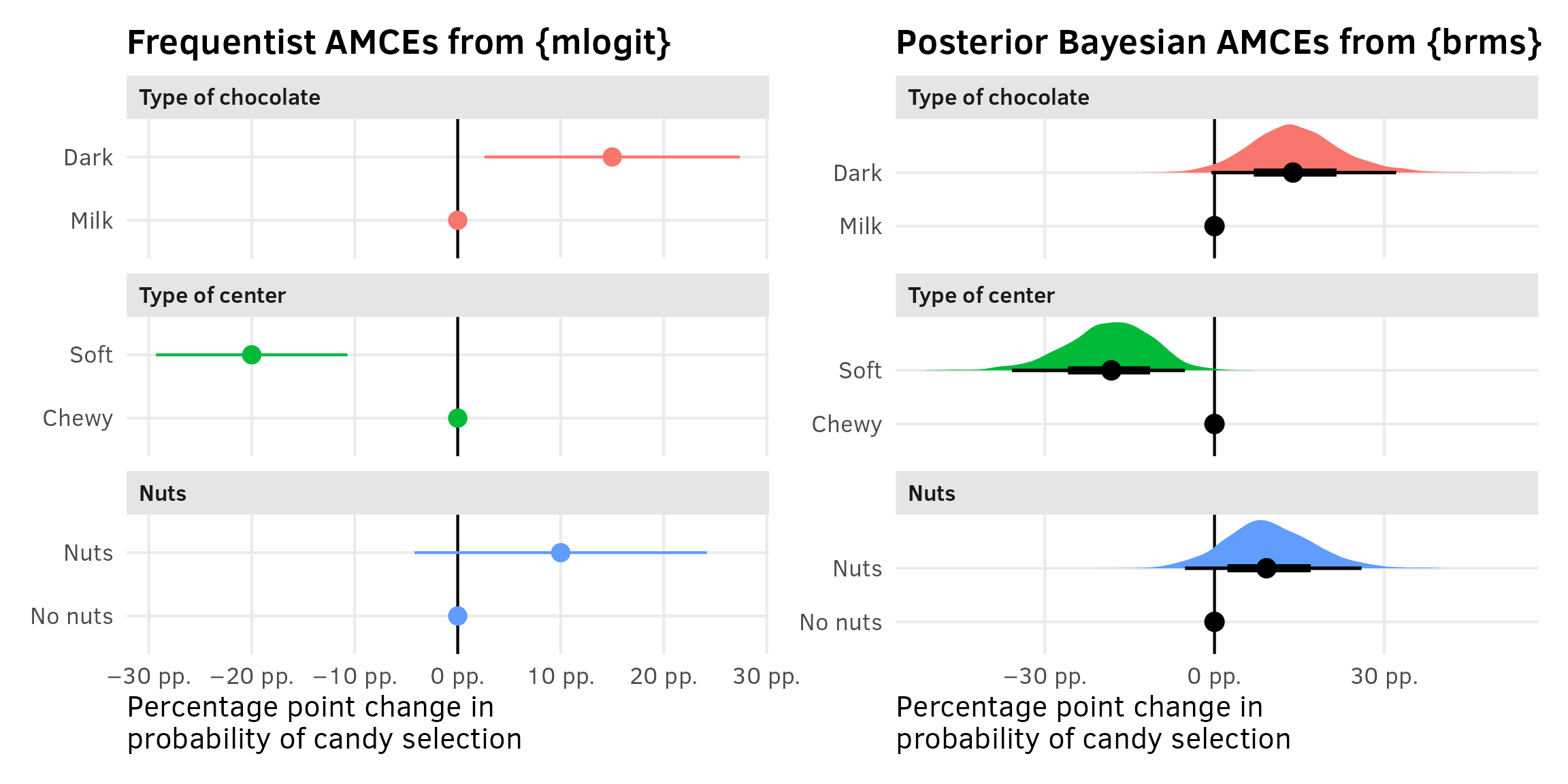

Example 2:

The setup

The data

The model

Predictions

AMCEs

Example 3:

The setup

The data

The model

Predictions

AMCEs

Footnotes

See here for an illustration of the relationship between multinomial and Poisson distributions; or see this 2011 Biometrika paper about using Poisson models to reduce bias in multinomial logit models.↩︎

Example 1: Basic multinomial logit with chocolate candy

The setup

The data

The model

Original SAS model as a baseline

Survival model

Poisson model

mlogit model

Bayesian model

Predictions

Frequentist predictions

Bayesian predictions

Plots

AMCEs

Bayesian comparisons/contrasts

Frequentist comparisons/contrasts

Plots

Example 2:

The setup

The data

The model

Predictions

AMCEs

Example 3:

The setup

The data

The model

Predictions

AMCEs

Footnotes

`mlogit` model