
| Variable | Description | Source |
|---|---|---|
| Pandemic Backsliding Index (PanBack) | 0–1; higher values represent greater risk of backsliding; ≥ 0.3 considered high risk | Varieties of Democracy PanDem |
| ICCPR derogation | Binary indicator | UN Treaty Collection |
| New and cumulative COVID deaths and cases | Counts | World Health Organization |
| Rule of law index | 0–1; higher values represent greater respect for rule of law | Varieties of Democracy |
| Emergency public health measures | Binary indicator | Oxford COVID-19 Government Response Tracker |
| Human rights and policy outcomes | Ordered categories for the severity of abuses | Varieties of Democracy PanDem |
Online appendix for “Derogations, Democratic Backsliding, and International Human Rights During the COVID-19 Pandemic”
Variable descriptions
Modeling approach
We use Stan 2.36.0 (Stan Development Team, 2023) through R 4.4.1 (R Core Team, 2024) and {brms} 2.21.0 (Bürkner, 2017) to estimate our models. We generate 4 MCMC chains for each model with 2,000 iterations in each chain, 1,000 of which are used for warmup. All chains converge; we assess convergence with visual inspection. Complete results from all the models, along with posterior predictive checks, goodness-of-fit measures, and prediction diagnostics are all available at a companion statistical analysis compendium at https://doi.org/10.17605/OSF.IO/ANONYMIZED-FOR-NOW.
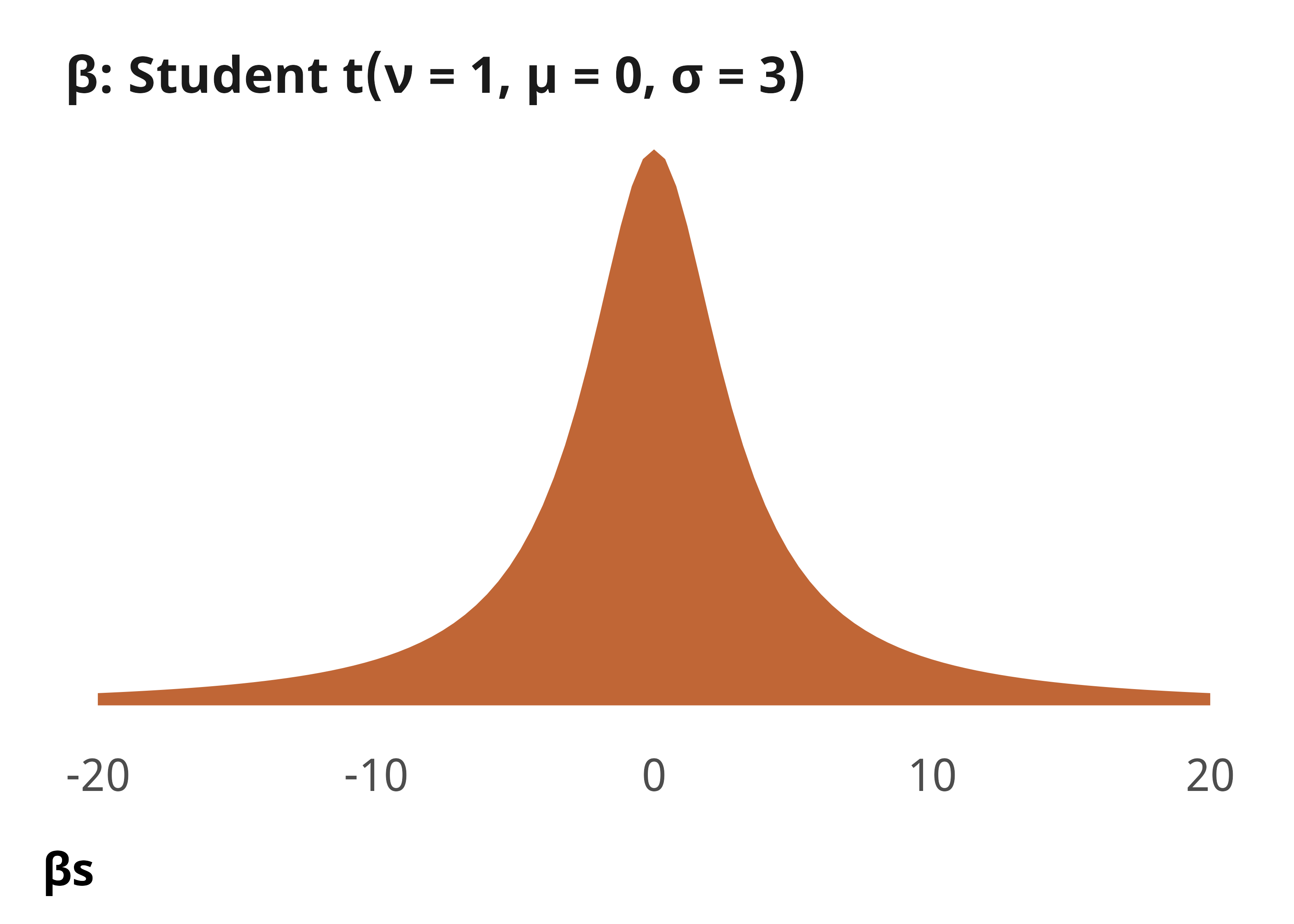
We use weakly informative priors (Gelman et al., 2008) for our logistic and ordered logistic regression models. For consistency with prior specification, and for computation efficiency, we mean-center all nonbinary variables so that parameter estimates represent changes from the mean. For all \(\beta\) terms in each of the models, we use a Student t distribution with a mean of 0 and a standard deviation of 3 (see Figure A1). This keeps most parameter estimates around −5 to 5, with thicker tails that allow for some possibility of extreme values. These priors give more weight to realistic areas of parameter values and downweight values in unrealistic spaces. For instance, since logit-scale coefficient values greater than 4 or 5 are highly unlikely, our Student t prior puts more weight on smaller values. Additionally, weakly informative priors allow reasonable and considerable uncertainty in possible parameter estimates.
Complete model results
The actual R code for these models is included in the replication code at https://doi.org/10.17605/OSF.IO/ANONYMIZED-FOR-NOW. We include a simplified representation of the {brms} (Bürkner, 2017) model code in each section below.
Explaining COVID-19 derogations
Formal model specification
\[ \begin{aligned} &\ \mathrlap{\textbf{Binary outcome $i$ across week $t$}} \\ \text{Treaty action}_{it_j} \sim&\ \operatorname{Bernoulli}(\pi_{it_j}) \\[0.75em] &\ \textbf{Distribution parameters} \\ \pi_{it} =&\ \beta_0 + \beta_1\ \text{PanBack}_{it} + \\ &\ \beta_2\ \text{New cases}_{it}\ + \beta_3\ \text{Cumulative cases}_{it}\ + \\ &\ \beta_4\ \text{New deaths}_{it}\ + \beta_5\ \text{Cumulative deaths}_{it}\ + \\ &\ \beta_6\ \text{Rule of law index}_{it}\ + \beta_7\ \text{Week number}_{it} \\[0.75em] &\ \textbf{Priors} \\ \beta_{0 \dots 7} \sim&\ \operatorname{Student\ t}(\nu = 1, \mu = 0, \sigma = 3) \end{aligned} \]
Simplified R code
brm(
  bf(outcome ~ panback +
      new_cases_z + cumulative_cases_z +
      new_deaths_z + cumulative_deaths_z +
      v2x_rule + year_week_num),
  family = bernoulli(),
  prior = c(
    prior(student_t(1, 0, 3), class = Intercept),
    prior(student_t(1, 0, 3), class = b)),
  ...
)
Complete results
| ICCPR action | ||
|---|---|---|
| Derogation filed | Other action | |
| Note: Estimates are median posterior log odds from logistic regression models; 95% credible intervals (highest density posterior interval, or HDPI) in brackets. | ||
| Pandemic backsliding (PanBack) | 1.35 | -2.5 |
| [-0.44, 3.11] | [-8.0, 1.9] | |
| New cases (standardized) | -1.41 | -0.47 |
| [-3.41, 0.34] | [-1.89, 0.65] | |
| New deaths (standardized) | 0.469 | -0.068 |
| [0.027, 0.917] | [-1.010, 0.745] | |
| Cumulative cases (standardized) | -2.05 | -0.56 |
| [-4.96, -0.17] | [-1.41, 0.31] | |
| Cumulative deaths (standardized) | 1.03 | 0.64 |
| [0.45, 1.69] | [-0.16, 1.34] | |
| Rule of law index | 0.45 | 3.2 |
| [-0.41, 1.26] | [1.2, 5.5] | |
| Year-week number | -0.0230 | 0.0097 |
| [-0.0369, -0.0089] | [-0.0156, 0.0324] | |
| Intercept | -5.1 | -8.6 |
| [-5.9, -4.1] | [-11.0, -6.5] | |
| N | 9591 | 9591 |
| \(R^2\) | 0.01 | 0.00 |
Model 2 in Table A2 presents the results of modeling the determinants of non-derogation treaty actions. This outcome is coded as 0 each country-week if a state did not issue one of these actions that week, and 1 that week if the state did. It is coded dichotomously rather than as a count because only three country-weeks non-derogation counts greater than 1 (these were country-weeks wherein Oman issued two, the UK two, and the UK three). The dichotomous coding also mirrors how we measured ICCPR derogation data in earlier models.
Explaining COVID-19 restrictions
Formal model specification
\[ \begin{aligned} &\ \mathrlap{\textbf{Model of outcome level $i$ across week $t$}} \\ \text{Outcome}_{it_j} \sim&\ \operatorname{Ordered\ logit}(\phi_{it_j}, \alpha_k) \\[0.75em] &\ \textbf{Distribution parameters} \\ \phi_{it} =&\ \beta_0 + \beta_1\ \text{PanBack (binary)}_{it} + \beta_2\ \text{Derogation in effect}_{it} + \\ &\ \beta_3\ [\text{PanBack (binary)}_{it} \times \text{Derogation in effect}_{it}] + \\ &\ \beta_4\ \text{New cases}_{it}\ + \beta_5\ \text{Cumulative cases}_{it}\ + \\ &\ \beta_6\ \text{New deaths}_{it}\ + \beta_7\ \text{Cumulative deaths}_{it}\ + \\ &\ \beta_8\ \text{Rule of law index}_{it}\ + \beta_9\ \text{Week number}_{it} \\[0.75em] &\ \textbf{Priors} \\ \beta_{0 \dots 9} \sim&\ \operatorname{Student\ t}(\nu = 1, \mu = 0, \sigma = 3) \\ \alpha_k \sim&\ \mathcal{N}(0, 1) \end{aligned} \]
Simplified R code
brm(
  bf(outcome ~ derogation_ineffect*panbackdichot +
      new_cases_z + cumulative_cases_z +
      new_deaths_z + cumulative_deaths_z +
      v2x_rule + year_week_num),
  family = cumulative(),
  prior = c(
    prior(student_t(1, 0, 3), class = Intercept),
    prior(student_t(1, 0, 3), class = b)),
  ...
)
Complete results
| Restricted movement | Close public transit | Stay at home | |
|---|---|---|---|
| Note: Estimates are median posterior log odds from ordered logistic regression models; 95% credible intervals (highest density posterior interval, or HDPI) in brackets. | |||
| Derogation in effect | 1.09 | 1.1 | 1.9 |
| [0.84, 1.30] | [0.9, 1.3] | [1.7, 2.1] | |
| Pandemic backsliding (PanBack), dichotomous | 0.61 | 0.75 | 1.11 |
| [0.45, 0.77] | [0.61, 0.91] | [0.95, 1.27] | |
| Derogation in effect × Pandemic backsliding | 0.99 | 0.11 | -0.44 |
| [-0.12, 2.28] | [-0.44, 0.75] | [-1.02, 0.16] | |
| New cases (standardized) | 0.59 | -0.092 | 0.016 |
| [0.34, 0.83] | [-0.176, -0.015] | [-0.072, 0.113] | |
| New deaths (standardized) | 0.42 | 0.24 | 0.33 |
| [0.22, 0.60] | [0.16, 0.32] | [0.25, 0.42] | |
| Cumulative cases (standardized) | -0.70 | -0.038 | -0.065 |
| [-0.90, -0.49] | [-0.142, 0.062] | [-0.174, 0.054] | |
| Cumulative deaths (standardized) | 0.81 | 0.146 | 0.072 |
| [0.59, 1.04] | [0.045, 0.255] | [-0.044, 0.186] | |
| Rule of law index | -0.55 | -0.81 | -0.38 |
| [-0.68, -0.42] | [-0.94, -0.68] | [-0.50, -0.26] | |
| Year-week number | -0.021 | -0.0113 | -0.00061 |
| [-0.023, -0.019] | [-0.0133, -0.0093] | [-0.00247, 0.00137] | |
| Cut 1 | -1.6 | -0.94 | -1.2 |
| [-1.8, -1.5] | [-1.06, -0.83] | [-1.3, -1.1] | |
| Cut 2 | -0.84 | 0.89 | 0.038 |
| [-0.96, -0.72] | [0.78, 1.01] | [-0.068, 0.144] | |
| Cut 3 | 2.8 | ||
| [2.7, 3.0] | |||
| N | 9591 | 9591 | 9591 |
| \(R^2\) | 0.11 | 0.07 | 0.09 |
Explaining COVID-19 human rights violations
Formal model specification
\[ \begin{aligned} &\ \mathrlap{\textbf{Model of outcome level $i$ across week $t$}} \\ \text{Outcome}_{it_j} \sim&\ \operatorname{Ordered\ logit}(\phi_{it_j}, \alpha_k) \\[0.75em] &\ \textbf{Distribution parameters} \\ \phi_{it} =&\ \beta_0 + \beta_1\ \text{PanBack (binary)}_{it} + \beta_2\ \text{Derogation in effect}_{it} + \\ &\ \beta_3\ [\text{PanBack (binary)}_{it} \times \text{Derogation in effect}_{it}] + \\ &\ \beta_4\ \text{New cases}_{it}\ + \beta_5\ \text{Cumulative cases}_{it}\ + \\ &\ \beta_6\ \text{New deaths}_{it}\ + \beta_7\ \text{Cumulative deaths}_{it}\ + \\ &\ \beta_8\ \text{Rule of law index}_{it}\ + \beta_9\ \text{Week number}_{it} \\[0.75em] &\ \textbf{Priors} \\ \beta_{0 \dots 9} \sim&\ \operatorname{Student\ t}(\nu = 1, \mu = 0, \sigma = 3) \\ \alpha_k \sim&\ \mathcal{N}(0, 1) \end{aligned} \]
Simplified R code
brm(
  bf(outcome ~ derogation_ineffect*panbackdichot +
      new_cases_z + cumulative_cases_z +
      new_deaths_z + cumulative_deaths_z +
      v2x_rule + year_week_num),
  family = cumulative(),
  prior = c(
    prior(student_t(1, 0, 3), class = Intercept),
    prior(student_t(1, 0, 3), class = b)),
  ...
)
Complete results
| Discriminatory policy | Non-derogable rights | Abusive enforcement | No time limits | Media restrictions | |
|---|---|---|---|---|---|
| Note: Estimates are median posterior log odds from logistic and ordered logistic regression models; 95% credible intervals (highest density posterior interval, or HDPI) in brackets. | |||||
| Derogation in effect | -0.45 | -4.1 | 1.09 | -1.6 | -1.5 |
| [-0.84, -0.11] | [-9.6, -1.4] | [0.91, 1.28] | [-2.0, -1.2] | [-1.7, -1.2] | |
| Pandemic backsliding (PanBack), dichotomous | 2.2 | 2.9 | 2.7 | 0.30 | 1.8 |
| [2.1, 2.4] | [2.7, 3.1] | [2.6, 2.9] | [0.12, 0.47] | [1.6, 2.1] | |
| Derogation in effect × Pandemic backsliding | -8.5 | 3.9 | -1.9 | 1.07 | 6.62 |
| [-54.4, -2.0] | [1.0, 9.5] | [-2.4, -1.4] | [0.25, 1.89] | [0.59, 46.63] | |
| New cases (standardized) | 0.0897 | -0.066 | 0.013 | -0.116 | 0.19 |
| [-0.0016, 0.1801] | [-0.352, 0.242] | [-0.059, 0.091] | [-0.287, 0.021] | [0.11, 0.30] | |
| New deaths (standardized) | -0.23 | -0.331 | -0.013 | 0.1121 | -0.15 |
| [-0.35, -0.11] | [-0.627, -0.042] | [-0.095, 0.078] | [0.0052, 0.2310] | [-0.24, -0.06] | |
| Cumulative cases (standardized) | 0.36 | -0.017 | 0.121 | -0.51 | 0.141 |
| [0.20, 0.53] | [-0.382, 0.340] | [0.011, 0.249] | [-0.70, -0.30] | [0.024, 0.263] | |
| Cumulative deaths (standardized) | -0.286 | -0.026 | -0.029 | 0.39 | -0.080 |
| [-0.478, -0.098] | [-0.397, 0.330] | [-0.153, 0.094] | [0.24, 0.55] | [-0.200, 0.029] | |
| Rule of law index | 0.69 | -0.64 | -1.11 | -0.34 | -5.2 |
| [0.48, 0.90] | [-0.95, -0.32] | [-1.26, -0.95] | [-0.50, -0.18] | [-5.3, -5.0] | |
| Year-week number | -0.0091 | -0.0014 | -0.024 | 0.0042 | -0.016 |
| [-0.0123, -0.0061] | [-0.0058, 0.0028] | [-0.026, -0.021] | [0.0017, 0.0065] | [-0.018, -0.013] | |
| Intercept | -2.8 | -1.08 | |||
| [-3.0, -2.5] | [-1.21, -0.95] | ||||
| Cut 1 | 2.2 | -0.182 | -4.3 | ||
| [2.1, 2.4] | [-0.305, -0.058] | [-4.5, -4.1] | |||
| Cut 2 | 2.9 | 0.91 | -4.0 | ||
| [2.8, 3.1] | [0.78, 1.04] | [-4.1, -3.8] | |||
| Cut 3 | 3.1 | 2.5 | -3.7 | ||
| [2.9, 3.3] | [2.3, 2.6] | [-3.9, -3.5] | |||
| N | 9591 | 9591 | 9591 | 9496 | 9591 |
| \(R^2\) | 0.12 | 0.16 | 0.23 | 0.02 | 0.42 |
Comparing COVID-19 derogations with other treaty actions
Figure A2 (also Figure 4 in the text of the paper) plots treaty actions by state and compares counts of derogations against other types of treaty actions. There were 42 states that issued any kind of human rights treaty action during this period. Twenty-one issued only derogations. The “super derogating states” that issued multiple derogations during this period also did not issue other types of treaty actions. For example, Peru issued 18 derogations and Guatemala 13, but neither of these states issued any other type of human rights treaty action during this period. Similarly, there were states that never issued derogations during this period but issued other types of human rights treaty actions. For example, the United Kingdom issued six, Oman issued three, and the Netherlands issued two other treaty actions.
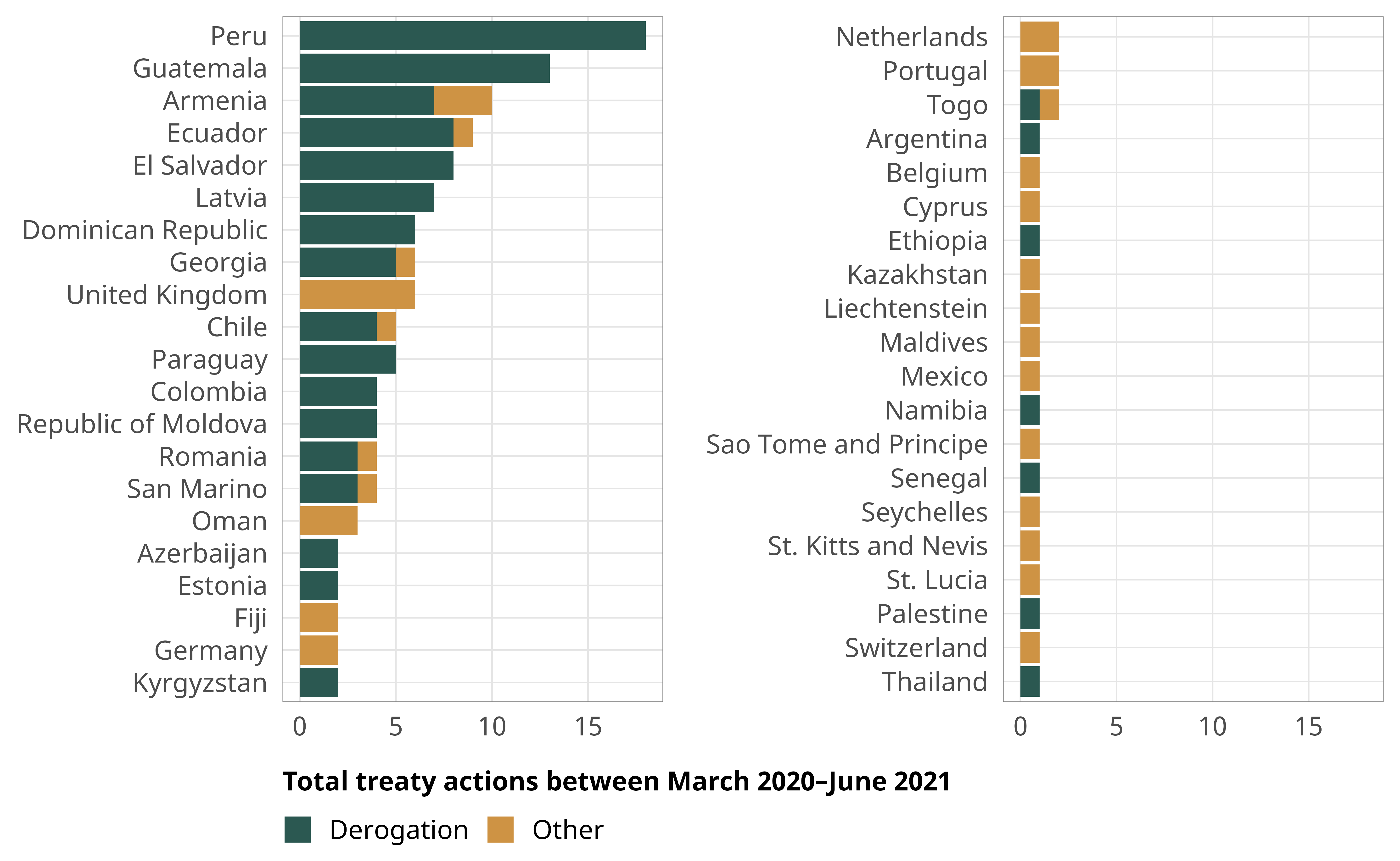
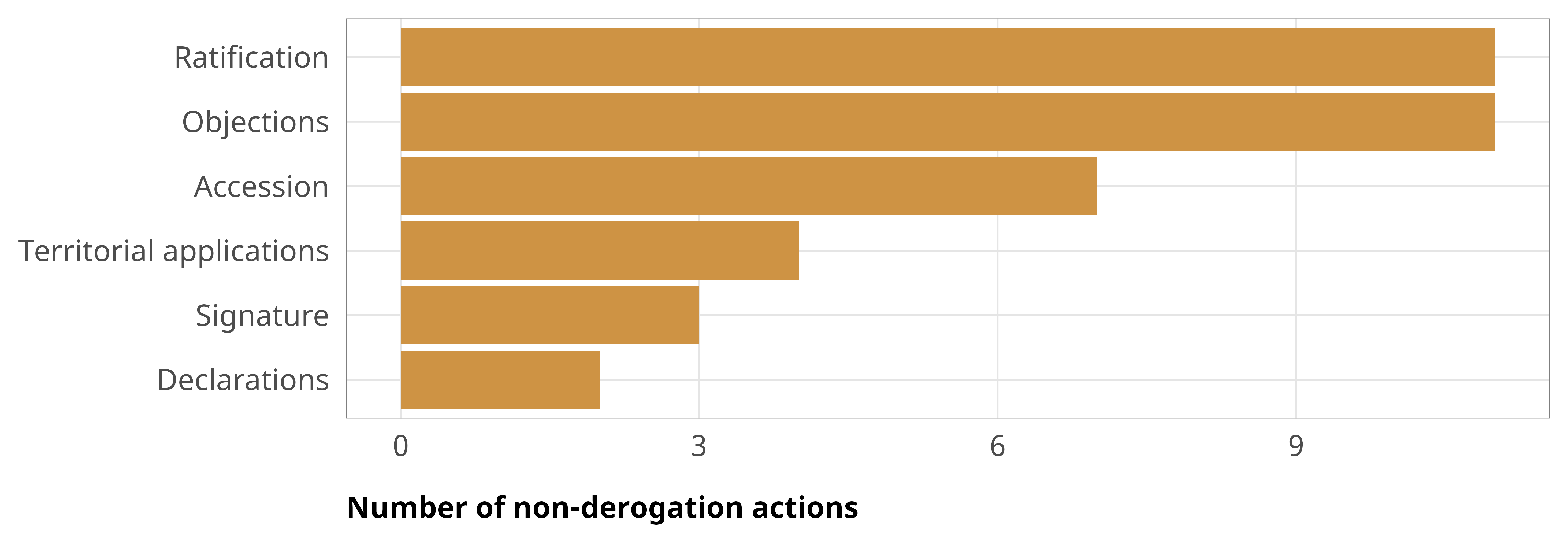
During this time, states issued treaty actions towards eight treaties and seven Optional Protocols, as shown in Table A5. Derogations to the ICCPR constituted the clear majority of United Nations human rights treaty engagement, comprising 111 of the 150 treaty actions. The remaining actions are depicted in Figure A3. The other actions were commitment actions (11 Ratifications; 7 Accessions; and 3 Signatures) and post-commitment actions (11 Objections; 4 Territorial Applications; and 2 Declarations). Of these actions, the Territorial Applications were similar to derogations in that they remove obligations from states to comply with elements of human rights treaties. Rather than highlighting specific articles and time dimensions of limited obligation like in derogations, territorial applications are geographic-based considerations of state obligation (Comstock, 2019). Territorial applications can remove or extend state obligations. The four territorial applications under consideration here were all issued by the United Kingdom and all extended state obligations of treaty ratification obligation to Bailiwick of Jersey, Guernsey, and Alderney, all island dependencies of the British Crown.
| Number of Actions | Treaties |
|---|---|
| 111 | ICCPR |
| 8 | CED |
| 7 | UN CRC Optional Protocol on the Involvement of Children in Conflict |
| 3 | CRPD OP; ICESCR OP |
| 2 | CAT; CRPD; ICCPR OP Abolition of Death Penalty; UN CRC Optional Protocol on the Sale of Chldren, Child Pornography, and Child Prostitution; UN CRC Optional Protocol Communications Procedure |
| 1 | CEDAW; CEDAW Amendment; CEDAW OP; CMW; Convention on the Non-Applicability of Statutory Limitations to War Crimes and Crimes Against Humanity; ICESCR; UN CRC |
Case study details
All of the states that experienced high risk of democratic backsliding and issued derogations were from the Central American or South America regions. The states that issued derogations but did not experience a high risk of democratic backsliding were from a mix of regions including South America, Central America, Asia, Eastern Europe, and Africa. In addition to the ICCPR, states also derogated from regional human rights treaties—the American Convention on Human Rights (ACHR) and the European Convention on Human Rights (ECHR) (Istrefi & Humburg, 2020). Therefore, the mini-cases below examine derogations to the ICCPR, as well as the ACHR and ECHR, where applicable.
High risk of backsliding, Derogations present: Guatemala
On March 9, 2020, Guatemala became the first state to formally derogate from Articles 12 and 21 of the ICCPR, both of which concern the freedoms of movement, association, assembly and demonstration (Peaceful Assembly Worldwide, 2021). Guatemala also sent official notification of derogation to the Organization of American States (OAS) on March 23, 2020, stating the government’s intention to derogate from Articles 15 and 22 of the ACHR (Ministerio de Relaciones Exteriores de Guatemala, 2020). Article 15 guarantees the right of peaceful assembly, while Article 22 protects the freedom of movement and residence. Counter to trends in many countries across the globe, Guatemala notified the ICCPR before it sent notifications of derogation to the OAS, demonstrating a clear commitment to the treaties and international law. In addition, from the 10 states that derogated from the ACHR, only 4, including Guatemala filed notification of derogations from the ICCPR (Istrefi & Humburg, 2020).
President Alejandro Giammattei was sworn in as President of Guatemala shortly before the pandemic. Prior democratic governments failed to meet their mandate—in 2019, more than half of the population lived below the poverty line (Freeman & Perelló, 2023). Corruption was another big concern—in January 2020, Transparency International ranked Guatemala as the fourth most corrupt country in the world. Holding office was often seen as lucrative not just for politicians but also for those financing these leaders (Freeman & Perelló, 2023). Thus, while many domestic and international observers were concerned about backsliding during his government, the pandemic also exacerbated fears about the relationship between transparency and corruption.
During the pandemic, Guatemala maintained a low rate of contagion compared with many other Latin American countries—which the government used to bolster its popularity. The OHCHR even praised the work done by the Office of Indigenous Women and the Ministry of Education for increasing support for indigenous children’s participation in primary education. Between 2020–2023, there was a 7% increase in enrollment (49% of which was among girls); moreover, the dropout rates decreased by 4% counter to global trends during the pandemic (OHCHR, 2023). In January 2021, the Guatemalan government requested derogations from two additional articles of the ACHR (Articles 13 and 16), and extensions to their previous derogations from Articles 15 and 22. Article 16 of the ACHR—like Article 21 of the ICCPR—protects the freedom of association, while Article 13 protects the freedom of thought and expression. Guatemala’s derogation from articles regarding freedom of thought and expression has been seen by some as a concerning attempt to silence media criticisms of the government’s handling of the pandemic (The Global State of Democracy Initiative, 2021). Human Rights Watch accused the administration of hindering journalists’ access to public information (Mercadal, 2024). This limited transparency also raised concerns about media freedom—though the government itself has not targeted any journalists, the media was shut out of various congressional sessions, making it unable to report accurately on the pandemic. Overall, though there were still causes for concern, Guatemala’s derogations seemed to be lawful and generally proportionate, and the government engaged in fewer rights violations than expected. The Central American nation was quick to communicate its intentions to its treaty organizations, and in this case, the government’s desire to communicate its intentions and maintain transparency may have provided a check on the rate of backsliding.
However, corruption was considered to be the main reason undermining efforts to fight the pandemic. Scholars noted that corruption during the pandemic “contributed to a regression of democracy” (Mercadal, 2024, p. 225). Concerns about democratic backsliding ultimately did not fully materialize—in August 2023, Bernardo Arévalo, a centrist anti-corruption reformer, won Guatemala’s presidential runoff by a wide margin after an electoral process that nearly saw Arévalo’s party barred from competing.
High risk of backsliding, no derogation: India
To illustrate the interaction of a high risk of democratic backsliding and the lack of derogations during the pandemic, we look at the case of India. According to Article 352 of India’s constitution, India is only allowed to declare a state of emergency when its territory is threatened “by war or external aggression or armed rebellion” (Constitution of India, n.d.)—not in the case of public health crises. Despite having an extremely deadly Delta wave of Covid-19 cases during the pandemic and the implementation of multiple measures to protect a sixth of the world’s population, India did not derogate from any treaties. Without derogations, there is an absence of sunset clauses that typically ensure that there is an end to the measures a country implements during an emergency. Thus, many measures disregarded ICCPR provisions that should have been protected even in a state of emergency.
When India went into lockdown in March 2020, the government only provided a four-hour notice—this violated ICCPR Article 19, the right to seek and receive information, including early warnings of national measures like the lockdown. Further, the CESCR General Comment No. 14 says that “access to information concerning the main health problems in the community, including methods of preventing and controlling them” is also a guaranteed right (Amnesty International, 2020). The lack of notice stranded a large number of migrant workers in cities, far from their homes in rural areas, with no transportation. Many of these workers died while trying to walk hundreds of miles back to their villages (Chaudhry & Prasad, 2020).
As the pandemic progressed, the Bharatiya Janata Party (BJP)-led government used the pandemic measures to hasten backsliding. The government paid little heed to technical and scientific advice (Mukherji, 2020). Instead, the BJP government used its institutional power to shut down dissent, especially from media, civil society, and lawyers. For instance, many measures disproportionately impacted journalists’ ability to work (ICNL, 2021). While these measures may have been intended to prevent misinformation, they were used to suppress journalists and activists. The government also used restrictions to arbitrarily arrest and detain opponents to the regime—including those protesting the government and its Hindu nationalist policies (Yasir & Schultz, 2020). Subsequent to their arrest, detainees had limited access to legal counsel, which led to their continued detention. Many measures also violated the right to privacy. Concerns over enhanced surveillance techniques arose after multiple leaks of personal information of infected peoples which has led to discrimination and even assault. These measures led to cases of Muslims being assaulted, harassed, and denied medical attention or spikes in caste-based discrimination and violence during the pandemic (Ayyub, 2020). Ultimately, many scholars and policymakers argued that these measures were used to tighten both the government’s grip on media as well as provide a justification to centralize power (Mukherji, 2020).
In The Global State of Democracy 2021 Report, India had the most violations among democracies experiencing backsliding. In the same year, Varieties of Democracy relegated India as an “electoral autocracy,” CIVICUS coded India’s civil society environment as “repressed,” and Reporters Without Borders in its World Press Freedom Index ranked India 161 out of 180 countries (Tripathi, 2023). Thus, over the course of the pandemic, India did not derogate from its treaty obligations, and its pandemic measures were further used to tighten both the government’s grip on the media as a justification to centralize power. These developments occurred in the context of India continuing to maintain an independent relationship with Russia, despite pressure from the West. India repeatedly abstained from UN resolutions condemning Russia, and India’s oil imports from Russia also increased after Western sanctions against the country (Grossman, 2022a). Thus, analysts have noted that while India is not abandoning the liberal international order, it has also ensured that by refusing to condemn Russia, it continues to receive tangible economic and security benefits from Russia (Grossman, 2022b).
Low risk of backsliding, issued derogations: Armenia
Armenia declared a state of emergency in March 2020 and promptly derogated from both the ICCPR and ECHR. The declaration of a state of emergency in Armenia through Decree No. 298-N on March 16, 2020, resulted in the suspension of certain constitutional rights and freedoms, including freedom of movement and peaceful assembly (ICNL, 2021). The derogations were later extended in accordance with international law. Armenia also officially notified the Secretary General of the Council of Europe (COE) of possible derogations from the obligations of Armenia under the Convention (Council of Europe, 2020a). On the 16th September 2020, Armenia withdrew all derogations and returned to full compliance with ICCPR (Peaceful Assembly Worldwide, 2021).
Unlike countries experiencing a high risk of backsliding, the Armenian government worked with civil society representatives and the media to formulate pandemic measures pertaining to them (Council of Europe, 2020b). These recommendations were subsequently incorporated into a government decree adopted on 24 March 2020, revising the restrictions, which was welcomed also by the Organisation for Security and Cooperation in Europe (OSCE) Media Freedom Representative, as well as commended by the Armenian media (Council of Europe, 2020b; OSCE, 2020). Furthermore, in its State Reply to the COE on April 13, 2020, the government declared that the restrictions of media activities became void. The rationale was that the Armenian government was highly confident “in the information on COVID-19 provided by official sources among population and a responsible behavior of the media during this period” (Council of Europe, 2020b). Thus, unlike many other countries, media restrictions were lifted shortly after the state emergency was declared.
Armenia’s derogations, and transparency not just with the treaty bodies, but also to the COE, as well as respect for media freedoms during this period can be explained, at least in part, by its increasing pivot to the West and desire to engage with the liberal international order. Russian-Armenian relations have been in decline, and there have been increasing discussions about Armenian desire to seek EU candidacy, breaking decades of affiliation with Russia (Castillo, 2024). After repeated Russian passivity over Azerbaijan’s offensives into Nagorno-Karabakh, Armenia froze relations with the Russian-led Collective Security Treaty Organization, organized military exercises with the US and expanded ties with democratic countries (Kucera, 2023). In December 2023, the Armenian Foreign Minister hoped that Armenia would, “get as close to the European Union as the EU deems possible” (Castillo, 2024).
Low risk of backsliding, no derogations: Hungary
Since taking office in 2010, Hungarian Prime Minister Viktor Orban implemented a number of constitutional and legal changes to consolidate his party’s control over the country’s institutions. In March 2020, in response to the pandemic, his government declared a national “State of Danger”—a special state of emergency (ICNL, 2021). Under this State of Danger, in addition to quarantining and social distancing regulations, and temporary closure of educational institutions, the government also increased police and military presence in the streets, border controls, and entry bans (ICNL, 2021). It also restricted data protection rights mandated by the General Data Protection Regulation (GDPR), an EU agreement that regulates information privacy. These restrictions allowed the government to use personal data of citizens without oversight (Massé et al., 2020). However, in implementing these measures, the government never notified the UN about its intent to derogate from the ICCPR.
The enforcement of these pandemic-related measures resulted in numerous violations of ICCPR and of derogation standards of non-discriminatory and proportional measures. In addition, many measures also restricted media freedom. Under one law, journalists who published “false” information about the pandemic or distorted government narratives would be punished with five years in jail (ICNL, 2021). The government also limited access to press conferences, only responded to media inquiries from pro-government outlets, and banned local health representatives from talking to the media (International Commission of Jurists, 2022). A 2022 report by the International Commission of Jurists on Hungary noted that, “By exercising emergency powers in order to justify the adoption of these measures, the government has failed to comply with or adequately consider international law standards with which such measures clearly conflict” (International Commission of Jurists, 2022). European Union Parliament lawmakers, in turn, demanded official punishment and denunciation of Hungary over some of these laws (Cox, 2020).
Hungary’s brazen violation of not just the ICCPR, but also European regulations such as the GDPR can be reflective of its increasing rift from the European Union (EU) and its pivot towards Russia. Hungary buys billions of dollars in Russian oil and gas, despite many in the West ceasing to do so after Russia’s invasion of Ukraine (Gavin et al., 2024). Unlike other countries that voluntarily divested from Russian gas, Hungary even struck new deals with Moscow (Gavin et al., 2024). Meanwhile, Orban has also criticized EU sanctions on Russia and blocked EU financial assistance for Ukraine (Ridgwell, 2024). However, Russia is not the only alternative source of goods for Hungary—more recently, China has filled in this role. In 2023, Hungary was among the largest global recipients of Chinese Belt and Road Initiative investment to finance a high-speed railway from Budapest to Serbia (Ridgwell, 2024). Thus, the presence of alternative patron states may have emboldened Hungary to violate not just international, but also European laws.
References
Amnesty International. (2020, March 16). Responses to COVID-19 and states’ human rights obligations: Preliminary observations [Press release]. https://www.amnestyusa.org/press-releases/responses-to-covid-19-and-states-human-rights-obligations-preliminary-observations/
Ayyub, R. (2020, April 6). Islamophobia taints India’s response to the coronavirus. Washington Post. https://www.washingtonpost.com/opinions/2020/04/06/islamophobia-taints-indias-response-coronavirus/
Bürkner, P.-C. (2017). brms: An R package for Bayesian multilevel models using Stan. Journal of Statistical Software, 80(1), 1–28. https://doi.org/10.18637/jss.v080.i01
Castillo, N. (2024, April 18). Armenia’s grand rebalance: EU and Russia. Caspian Policy Center. https://www.caspianpolicy.org/research/armenia/armenias-grand-rebalance-eu-and-russia
Chaudhry, S., & Prasad, S. K. (2020, March 30). How India plans to put 1.3 billion people on a coronavirus lockdown. Washington Post. https://www.washingtonpost.com/politics/2020/03/30/how-india-plans-put-13-billion-people-coronavirus-lockdown/
Comstock, A. L. (2019). Adjusted ratification: Post-commitment actions to UN human rights treaties. Human Rights Review, 20(1), 23–45. https://doi.org/10.1007/s12142-018-0536-0
Constitution of India. (n.d.). Proclamation of emergency (Part XVIII, article 352). https://www.constitutionofindia.net/articles/article-352-proclamation-of-emergency/
Council of Europe. (2020a). Armenia: Declaration related to the Convention for the Protection of Human Rights and Fundamental Freedoms (ETS No. 5) (JJ9015C Tr./005-227). Council of Europe Treaty Office. https://www.coe.int/en/web/conventions/derogations-covid-19
Council of Europe. (2020b, April 13). Armenian State reply to the alert “Emergency Restrictions Force Media to Suppress Independent Information on COVID-19”. https://rm.coe.int/armenia-reply-en-emergency-restrictions-force-media-to-suppress-indepe/16809e4ace
Cox, M. (2020). States of emergency and human rights during a pandemic: A Hungarian case study. Human Rights Brief, 24(1). https://digitalcommons.wcl.american.edu/hrbrief/vol24/iss1/5/
Freeman, W., & Perelló, L. (2023, August). A shock to Guatemala’s system. Journal of Democracy. https://www.journalofdemocracy.org/online-exclusive/a-shock-to-guatemalas-system/
Gavin, G., Jack, V., & Gijs, C. (2024, May 13). Hungary teases veto over new EU Russian gas sanctions. Politico. https://www.politico.eu/article/hungary-veto-eu-russia-gas-sanctions/
Gelman, A., Jakulin, A., Pittau, M. G., & Su, Y.-S. (2008). A weakly informative default prior distribution for logistic and other regression models. The Annals of Applied Statistics, 2(4). https://doi.org/10.1214/08-AOAS191
Grossman, D. (2022a, June 6). Modi’s multipolar moment has arrived. Foreign Policy. https://foreignpolicy.com/2022/06/06/modi-india-russia-ukraine-war-china-us-geopolitics-multipolar-quad/
Grossman, D. (2022b, December 9). India’s maddening Russia policy isn’t as bad as Washington thinks. Foreign Policy. https://foreignpolicy.com/2022/12/09/india-russia-ukraine-war-putin-modi-biden-sanctions-geopolitics/
ICNL. (2021). COVID-19 civic freedom tracker. https://www.icnl.org/covid19tracker/
International Commission of Jurists. (2022). A facade of legality: COVID-19 and the exploitation of emergency powers in Hungary. International Commission of Jurists. https://www.icj.org/wp-content/uploads/2022/02/Hungary-A-Facade-of-Legality-legal-briefing-2022-ENG.pdf
Istrefi, K., & Humburg, I. (2020, April 18). To notify or not to notify: Derogations from human rights treaties. Opinio Juris. https://opiniojuris.org/2020/04/18/to-notify-or-not-to-notify-derogations-from-human-rights-treaties/
Kucera, J. (2023, September 13). Is Armenia turning to the west? Radio Free Europe/Radio Liberty. https://www.rferl.org/a/armenia-pashinian-united-states-west-relations-russia-analysis/32591327.html
Massé, E., Szabó, M., & Dénes, B. (2020). Joint letter to the European Data Protection Board (EDPB) from Access Now, Hungarian Civil Liberties Union, and Civil Liberties Union for Europe. https://hclu.hu/en/articles/joint-letter-hungarian-govts-decision-to-limit-gdpr-rights-is-disproportionate-and-unjustified
Mercadal, T. (2024). The collective narratives of Covid-19 in Guatemala: The state, the church, the people. In A. Espinoza Carvajal & L. Medina Cordova (Eds.), Pandemic and Narration: Covid-19 Narratives in Latin America. Vernon Press.
Ministerio de Relaciones Exteriores de Guatemala. (2020). Suspensión de garantías constitucionales debido a la pandemia de COVID-19 (Ref. NV-OEA-M4-No.182-2020). Organization of American States. http://www.oas.org/es/sla/ddi/docs/tratados_multilaterales_suspencion_garantias_Guatemala_nota_No_182-2020.pdf
Mukherji, R. (2020). Covid vs. democracy: India’s Illiberal remedy. Journal of Democracy, 31(4), 91–105. https://doi.org/10.1353/jod.2020.0058
OHCHR. (2023). Experts of the Committee on the Elimination of Discrimination against Women welcome women’s increased participation in public life in Guatemala, ask the state about political violence and gender stereotyping [Press release]. Office of the High Commissioner for Human Rights. https://www.ohchr.org/en/news/2023/10/experts-committee-elimination-discrimination-against-women-welcome-womens-increased
OSCE. (2020). OSCE Media Freedom Representative welcomes swift reaction of Armenian Government in addressing his concerns on State of Emergency Decree [Press release]. Organization for Security and Co-operation in Europe. https://www.osce.org/representative-on-freedom-of-media/449290
Peaceful Assembly Worldwide. (2021). Derogations by States Parties from Article 21 ICCPR, Article 11 ECHR, and Article 15 ACHR on the Basis of the COVID-19 Pandemic. Centre for Human Rights, University of Pretoria. https://www.rightofassembly.info/assets/downloads/Derogations_by_States_Parties_from_the_right_to_assembly_on_the_Basis_of_the_COVID_19_Pandemic_(as_of_3_March_2021).pdf
R Core Team. (2024). R: A language and environment for statistical computing [Computer software]. R Foundation for Statistical Computing. https://www.r-project.org/
Ridgwell, H. (2024, February 23). Hungary appears to be strengthening ties with Russia, China. Voice of America. https://www.voanews.com/a/hungary-appears-to-be-strengthening-ties-with-russia-china/7499682.html
Stan Development Team. (2023). Stan Modeling Language (Version 2.26.1) [Computer software]. https://mc-stan.org
The Global State of Democracy Initiative. (2021). Guatemala (COVID-19). https://www.idea.int/gsod-indices/profile/covid19/guatemala
Tripathi, S. (2023, June 20). India’s worsening democracy makes it an unreliable ally. TIME. https://time.com/6288505/indias-worsening-democracy-makes-it-an-unreliable-ally/
Yasir, S., & Schultz, K. (2020, July 19). India rounds up critics under shadow of virus crisis, activists say. The New York Times. https://www.nytimes.com/2020/07/19/world/asia/india-activists-arrests-riots-coronavirus.html