Figures for “Global Assessment Power in the Twenty-First Century”
Judith Kelley and Beth Simmons
July 31, 2018
Data and code
Replication data and code available at GitHub.
library(tidyverse)
library(forcats)
library(stringr)
library(ggstance)
library(ggforce)
library(maptools)
library(rgdal)
library(scales)
library(zoo)

# Useful functions
theme_gpa <- function(base_size=10, base_family="Clear Sans") {
  update_geom_defaults("bar", list(fill = "grey30"))
  update_geom_defaults("line", list(colour = "grey30"))
  update_geom_defaults("label", list(family="Clear Sans"))
  update_geom_defaults("text", list(family="Clear Sans"))
  ret <- theme_bw(base_size, base_family) +
    theme(panel.background = element_rect(fill="#ffffff", colour=NA),
          axis.title.y = element_text(margin = margin(r = 10)),
          axis.title.x = element_text(margin = margin(t = 10)),
          axis.text = element_text(colour="black"),
          title=element_text(vjust=1.2, family="Clear Sans", face="bold"),
          plot.subtitle=element_text(family="Clear Sans"),
          plot.caption=element_text(family="Clear Sans",
                                    size=rel(0.8), colour="grey70"),
          panel.border = element_blank(),
          axis.line=element_line(colour="grey50", size=0.2),
          #panel.grid=element_blank(),
          axis.ticks=element_blank(),
          legend.position="bottom",
          legend.title=element_text(size=rel(0.8)),
          axis.title=element_text(size=rel(0.8), family="Clear Sans", face="bold"),
          strip.text=element_text(size=rel(1), family="Clear Sans", face="bold"),
          strip.background=element_rect(fill="#ffffff", colour=NA),
          panel.spacing.y=unit(1.5, "lines"),
          legend.key=element_blank(),
          legend.spacing=unit(0.2, "lines"))

  ret
}

theme_blank_map <- function(base_size=9.5, base_family="Clear Sans") {
  ret <- theme_bw(base_size, base_family) +
    theme(panel.background = element_rect(fill="#ffffff", colour=NA),
          panel.border=element_blank(), axis.line=element_blank(),
          panel.grid=element_blank(), axis.ticks=element_blank(),
          axis.title=element_blank(), axis.text=element_blank())
  ret
}

fig.save.cairo <- function(fig, filepath=file.path(PROJHOME, "Output"),
                           filename, width, height, units="in", seed=NULL, ...) {
  if (!is.null(seed)) set.seed(seed)
  ggsave(fig, filename=file.path(filepath, paste0(filename, ".pdf")),
         width=width, height=height, units=units, device=cairo_pdf, ...)
  if (!is.null(seed)) set.seed(seed)
  ggsave(fig, filename=file.path(filepath, paste0(filename, ".png")),
         width=width, height=height, units=units, type="cairo", dpi=300, ...)
}

# Clean up the interval labels created by cut()
# Use with forcats::fct_relabel
clean.cut.range <- function(x) {
  # If the level starts with "(", strip all the ( and [s and add 1 to the first value
  need.to.clean <- str_detect(x, "^\\(")
  cleaned <- str_replace_all(x[need.to.clean], "\\(|\\]", "") %>%
    map_chr(function(x) {
      x.split <- as.numeric(str_split(x, ",", simplify=TRUE))
      paste0(x.split[1] + 1, "–", x.split[2])
    })
}

my_percent <- percent_format(accuracy = 1)


# Load clean dataFigure 1: Cumulative number of GPAs.
year.chunks <- tribble(
  ~chunk_start, ~chunk_end, ~chunk_name,
  1900,         1969,       "Pre-1970",
  1970,         1974,       "1970–74",
  1975,         1979,       "1975–79",
  1980,         1984,       "1980–84",
  1985,         1989,       "1985–89",
  1990,         1994,       "1990–94",
  1995,         1999,       "1995–99",
  2000,         2004,       "2000–04",
  2005,         2009,       "2005–09",
  2010,         2014,       "2010–14",
  2015,         2020,       "2015+"
) %>%
  mutate(chunk_name = ordered(fct_inorder(chunk_name)))

year.chunks.long <- year.chunks %>%
  rowwise() %>%
  summarise(chunk_name = chunk_name, years = list(chunk_start:chunk_end)) %>%
  unnest()

years.active <- gpa.data.clean %>%
  filter(!is.na(start_year)) %>%
  rowwise() %>%
  summarise(gpa_id = gpa_id, years = list(start_year:recent_year),
            last.active = recent_year) %>%
  unnest() %>%
  mutate(active = TRUE)

gpas.active.over.time <- years.active %>%
  expand(gpa_id, years) %>%
  left_join(years.active, by=c("gpa_id", "years")) %>%
  group_by(gpa_id) %>%
  mutate(last.active = na.locf(last.active, na.rm=FALSE)) %>%
  # Get rid of rows with absolutely no data
  filter((!is.na(last.active) | !is.na(active))) %>%
  # Carry forward the active status of the last year marked if the GPA is still
  # active (i.e. last_active is >= 2014). Otherwise, mark as inactive and carry
  # forward.
  ungroup() %>%
  mutate(imputed.active = case_when(
    is.na(.$active) & .$last.active >= 2014 ~ TRUE,
    is.na(.$active) & .$last.active < 2014 ~ FALSE,
    TRUE ~ .$active
  )) %>%
  # Keep all active years; only keep the first inactive year
  group_by(gpa_id, imputed.active) %>%
  filter(imputed.active == TRUE |
           (imputed.active == FALSE & row_number() == 1)) %>%
  ungroup()

gpa.cum.plot <- gpas.active.over.time %>%
  left_join(year.chunks.long, by="years") %>%
  group_by(gpa_id, chunk_name, imputed.active) %>%
  slice(1) %>%
  group_by(chunk_name, imputed.active) %>%
  summarise(num = n()) %>%
  group_by(imputed.active) %>%
  # Calculate cumulative total
  mutate(cum_total = cumsum(num)) %>%
  ungroup() %>%
  # Only use cumulative total for inactive ones, since they drop out of the
  # data and aren't repeated like the active ones
  mutate(plot_value = ifelse(imputed.active, num, cum_total)) %>%
  mutate(active = factor(imputed.active, levels=c(TRUE, FALSE),
                         labels=c("Active GPIs in period", "Cumulative discontinued GPIs"),
                         ordered=TRUE)) %>%
  filter(chunk_name != "2015+")

gpas.active <- gpa.data.clean %>% filter(active == TRUE) %>% nrow
gpas.defunct <- gpa.data.clean %>% filter(active == FALSE) %>% nrow
Source: Authors’ database.
Note: “Active” denotes GPAs that were maintained in the given time period. GPAs that have not been updated since 2014 are marked as “Discontinued” in the year following the last active year.
N = 138 active GPAs in 2015; 21 total discontinued GPAs.
fig.cum.gpas <- ggplot(gpa.cum.plot, aes(x=chunk_name, y=plot_value)) +
  geom_col(data=filter(gpa.cum.plot, imputed.active), aes(fill=active)) +
  geom_line(data=filter(gpa.cum.plot, !imputed.active),
            aes(color=active, group=active), size=1) +
  scale_color_manual(values=c("grey30"), name=NULL) +
  scale_fill_manual(values=c("grey70"), name=NULL) +
  guides(fill=guide_legend(order=1),
         color=guide_legend(order=2)) +
  labs(x=NULL, y=NULL) +
  theme_gpa(9) + theme(legend.key.size=unit(0.65, "lines"),
                       legend.key=element_blank(), legend.spacing=unit(0, "lines"),
                       legend.margin = margin(0),
                       panel.grid.major.x=element_blank(),
                       panel.grid.minor.y = element_blank(),
                       legend.position = c(0.175, 0.9),
                       legend.background=element_blank())
fig.cum.gpas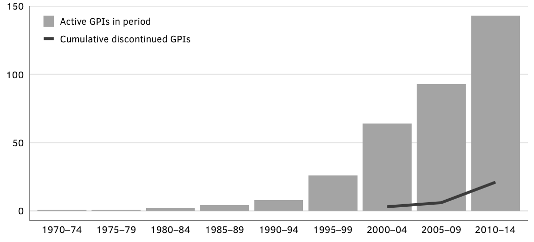
Collapsed subjects
Several of the smaller subject areas are collapsed into larger overarching categories, listed in the table below:
subjects_collapsed %>%
  select(`Subject (collapsed)` = subject_collapsed,
         `Subject (original)` = subject_area) %>%
pander::pandoc.table(justify = "ll")| Subject (collapsed) | Subject (original) |
|---|---|
| Education | Education |
| Development | Development |
| Economic | Economic |
| Environment | Environment |
| Environment | Energy |
| Governance | Governance |
| Human Rights | Gender |
| Human Rights | Human Rights |
| Human Rights | Press Freedom |
| Security | Security |
| Social | Social |
| Social | Health |
| Trade & Finance | Finance |
| Trade & Finance | Technology |
| Trade & Finance | Trade |
Figure 2 (new): Number of GPAs, by issue and creator type.
gpa.issues.creators <- gpa.data.clean %>%
  filter(active == 1, !is.na(subject_collapsed), !is.na(creator_collapsed)) %>%
  mutate(subject_collapsed = str_split(subject_collapsed, ", ")) %>%
  unnest(subject_collapsed) %>%
  group_by(creator_collapsed, subject_collapsed) %>%
  summarise(num = n()) %>%
  group_by(subject_collapsed) %>%
  mutate(total_in_group = sum(num)) %>%
  ungroup() %>%
  complete(subject_collapsed, creator_collapsed, fill=list(num = 0)) %>%
  arrange(total_in_group, num) %>%
  mutate(creator_collapsed = fct_relevel(creator_collapsed,
                                         c("Other", "University or Private",
                                           "State", "IGO", "NGO"))) %>%
  mutate(subject_collapsed = fct_inorder(subject_collapsed))

issue.creator.denominator <- gpa.data.clean %>%
  filter(active == 1, !is.na(creator_collapsed)) %>%
  nrow
Source: Authors’ database.
Note: Includes only “active” GPAs as of 2014; excludes defunct cases. Note that the total count of GPAs is larger than in Figure 1 because we have double counted cases that straddle issue areas, such as health and development. Overlapping and unknown creators are ommitted.
N = 138.
fig.by.issue.creator <- ggplot(gpa.issues.creators,
                               aes(x=num, y=subject_collapsed, fill=creator_collapsed)) +
  geom_barh(stat="identity", position=position_stackv()) +
  scale_x_continuous(sec.axis = sec_axis(~ . / issue.creator.denominator,
                                         labels=my_percent)) +
  # scale_fill_grey(start=0.9, end=0.2) +
  scale_fill_manual(values=rev(c("black", "grey50", "grey70", "grey25", "grey90"))) +
  guides(fill=guide_legend(reverse=TRUE, title=NULL, nrow=1)) +
  labs(x=NULL, y=NULL) +
  theme_gpa() + theme(panel.grid.major.y=element_blank())
fig.by.issue.creator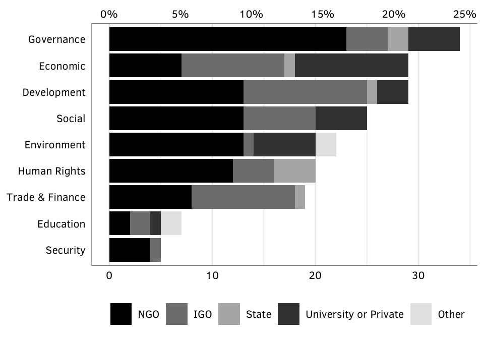
Figure 2: Number of GPAs, by issue.
gpa.issues <- gpa.data.clean %>%
  filter(active == 1, !is.na(subject_collapsed)) %>%
  mutate(subject_collapsed = str_split(subject_collapsed, ", ")) %>%
  unnest(subject_collapsed) %>%
  # Get a count of each collapsed issue
  group_by(subject_collapsed) %>%
  summarise(issue_count = n()) %>%
  ungroup() %>%
  arrange(issue_count) %>%
  mutate(subject_collapsed = fct_inorder(subject_collapsed))

issue.denominator <- gpa.data.clean %>%
  filter(active == 1, !is.na(subject_collapsed)) %>%
  nrow
Source: Authors’ database.
Note: Includes only “active” GPAs as of 2012; excludes defunct cases. Note that the total count of GPAs is larger than in Figure 1 because we have double counted cases that straddle issue areas, such as health and development.
N = 138 active GPAs.
fig.by.issue <- ggplot(gpa.issues, aes(x=issue_count, y=subject_collapsed)) +
  geom_barh(stat="identity") +
  scale_x_continuous(sec.axis = sec_axis(~ . / issue.denominator,
                                         labels=my_percent)) +
  labs(x=NULL, y=NULL) +
  theme_gpa() + theme(panel.grid.major.y=element_blank())
fig.by.issue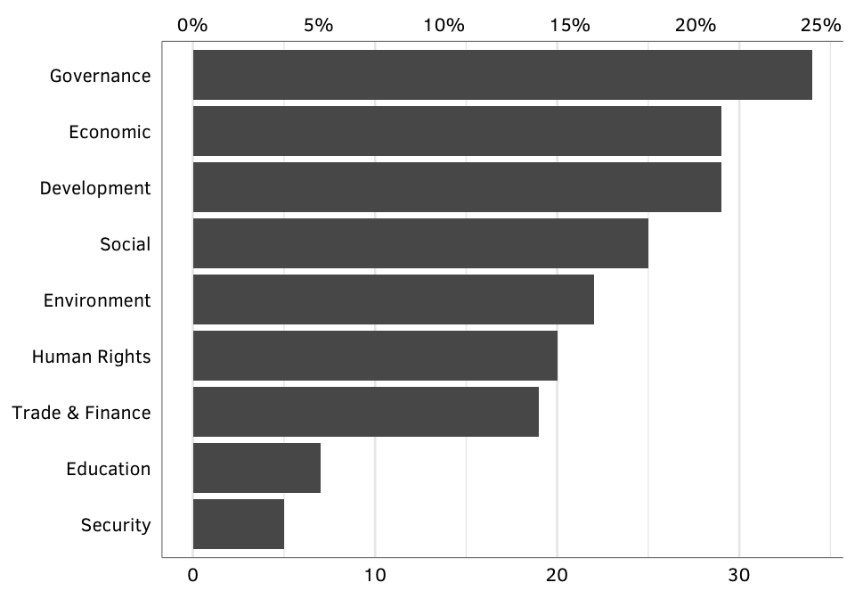
Figure 3: GPA creators, by type.
gpa.creators <- gpa.data.clean %>%
  filter(!is.na(creator_collapsed)) %>%
  group_by(creator_collapsed) %>%
  summarise(num = n()) %>%
  arrange(num) %>%
  mutate(creator_collapsed = str_replace(creator_collapsed,
                                         "ping or", "ping\nor")) %>%
  mutate(creator_collapsed = fct_inorder(creator_collapsed))

creator.denominator <- gpa.data.clean %>%
  filter(!is.na(creator_collapsed)) %>%
  nrow
Source: Authors’ database.
N = 159.
fig.by.creator <- ggplot(gpa.creators, aes(x=num, y=creator_collapsed)) +
  geom_barh(stat="identity") +
  scale_x_continuous(sec.axis = sec_axis(~ . / creator.denominator,
                                         labels=my_percent)) +
  labs(x=NULL, y=NULL) +
  theme_gpa() + theme(panel.grid.major.y=element_blank())
fig.by.creator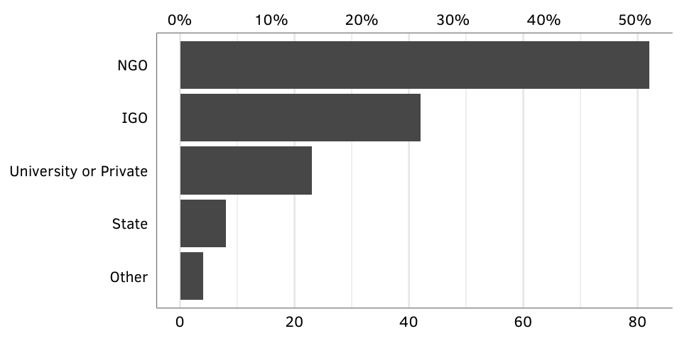
Figure X: GPA creators, by type (GPAs active as of 2014)
gpa.creators.active <- gpa.data.clean %>%
  filter(active) %>%
  filter(!is.na(creator_collapsed)) %>%
  group_by(creator_collapsed) %>%
  summarise(num = n()) %>%
  arrange(num) %>%
  mutate(creator_collapsed = str_replace(creator_collapsed,
                                         "ping or", "ping\nor")) %>%
  mutate(creator_collapsed = fct_inorder(creator_collapsed))

creator.active.denominator <- gpa.data.clean %>%
  filter(active) %>%
  filter(!is.na(creator_collapsed)) %>%
  nrow

creator.ngos <- gpa.creators.active %>%
  filter(creator_collapsed == "NGO") %>%
  select(num) %>% unname() %>% unlist() %>% c()

creator.ngos.pct <- my_percent(creator.ngos /
                                 creator.active.denominator)

creator.states.igos <- gpa.creators.active %>%
  filter(creator_collapsed %in% c("IGO", "State")) %>%
  summarise(num = sum(num)) %>%
  select(num) %>% unname() %>% unlist() %>% c()

creator.states.igos.pct <- my_percent(creator.states.igos /
                                        creator.active.denominator)
The figure below shows the distribution of the creator types among the currently active GPAs in our database, showing that 52% percent of GPAs are created by NGOs, while only 30% are in the direct control of states or IGOs.
Source: Authors’ database.
N = 138.
fig.by.creator.active <- ggplot(gpa.creators.active, aes(x=num, y=creator_collapsed)) +
  geom_barh(stat="identity") +
  scale_x_continuous(sec.axis = sec_axis(~ . / creator.active.denominator,
                                         labels=my_percent)) +
  labs(x=NULL, y=NULL) +
  theme_gpa() + theme(panel.grid.major.y=element_blank())
fig.by.creator.active
Figure 4: Country of GPA source headquarters.
gpa.countries <- gpa.data.clean %>%
  group_by(country_collapsed) %>%
  summarise(num = n()) %>%
  filter(!is.na(country_collapsed), country_collapsed != "Unknown") %>%
  arrange(num) %>%
  mutate(country_collapsed = fct_inorder(country_collapsed))

country.denominator <- sum(gpa.countries$num)
Source: Authors’ database.
N = 148.
fig.by.country <- ggplot(gpa.countries, aes(x=num, y=country_collapsed)) +
  geom_barh(stat="identity") +
  scale_x_continuous(sec.axis = sec_axis(~ . / country.denominator,
                                         labels=my_percent)) +
  labs(x=NULL, y=NULL) +
  theme_gpa() + theme(panel.grid.major.y=element_blank())
fig.by.country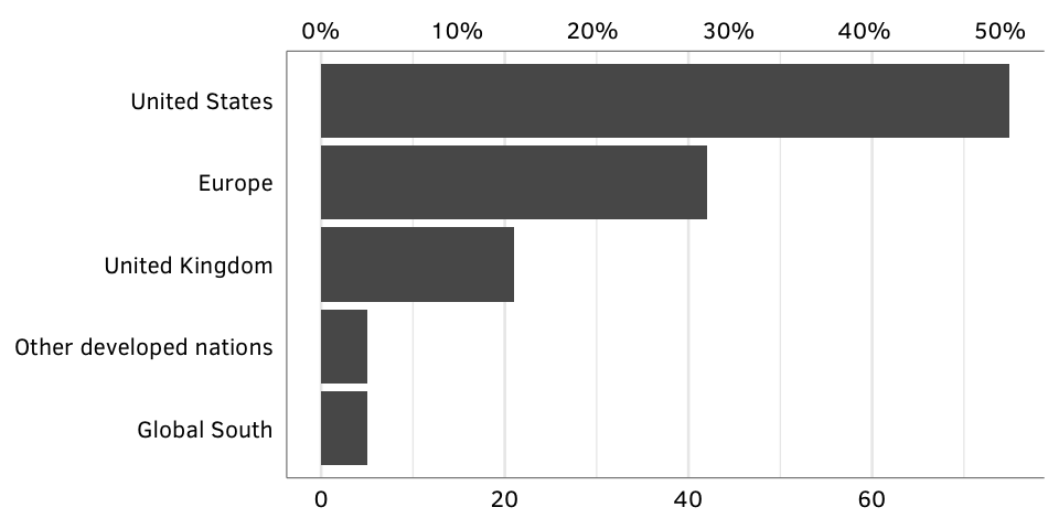
Figure 4: Country of GPA source headquarters (maps).
# Load map data
if (!file.exists(file.path(PROJHOME, "Data", "map_data",
                           "ne_110m_admin_0_countries.VERSION.txt"))) {
  map.url <- paste0("http://www.naturalearthdata.com/",
                    "http//www.naturalearthdata.com/download/110m/cultural/",
                    "ne_110m_admin_0_countries.zip")
  map.tmp <- file.path(PROJHOME, "Data", basename(map.url))
  download.file(map.url, map.tmp)
  unzip(map.tmp, exdir=file.path(PROJHOME, "Data", "map_data"))
  unlink(map.tmp)
}
countries.map <- readOGR(file.path(PROJHOME, "Data", "map_data"),
"ne_110m_admin_0_countries",
verbose=FALSE)
countries.robinson <- spTransform(countries.map, CRS("+proj=robin"))
countries.ggmap <- fortify(countries.robinson, region="iso_a3") %>%
filter(!(id %in% c("ATA", -99))) %>% # Get rid of Antarctica and NAs
mutate(id = ifelse(id == "GRL", "DNK", id)) # Greenland is part of Denmark
possible.countries <- data_frame(ISO3 = unique(as.character(countries.ggmap$id)))
gpa.countries.map <- gpa.data.clean %>%
group_by(ISO3) %>%
summarise(num = n()) %>%
filter(!is.na(ISO3)) %>%
# Bring in full list of countries and create new variable indicating if the
# country has any GPAs
right_join(possible.countries, by="ISO3") %>%
mutate(num.bin = !is.na(num),
num.ceiling = ifelse(num >= 10, 10, num))Source: Authors’ data
N = 17 countries.
gpa.map.bin <- ggplot(gpa.countries.map, aes(fill=num.bin, map_id=ISO3)) +
  geom_map(map=countries.ggmap, size=0.15, colour="black") +
  expand_limits(x=countries.ggmap$long, y=countries.ggmap$lat) +
  coord_equal() +
  scale_fill_manual(values = c("white", "grey30"), guide=FALSE) +
  theme_blank_map()
gpa.map.bin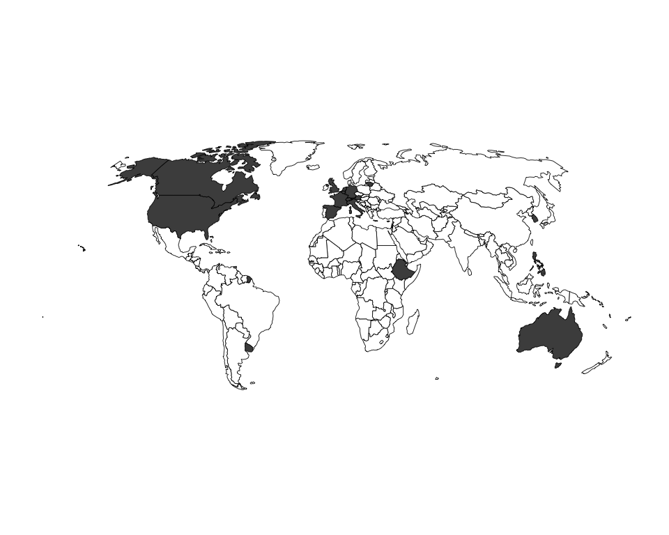
gpa.map <- ggplot(gpa.countries.map, aes(fill=num.ceiling, map_id=ISO3)) +
  geom_map(map=countries.ggmap, size=0.15, colour="black") +
  expand_limits(x=countries.ggmap$long, y=countries.ggmap$lat) +
  coord_equal() +
  scale_fill_gradient(low="grey90", high="grey30", breaks=seq(2, 10, 2),
                      labels=c(paste(seq(2, 8, 2), "  "), "10+"),
                      na.value="white", name="GPAs based in country",
                      guide=guide_colourbar(ticks=FALSE, barwidth=5)) +
  theme_blank_map(9) +
  theme(legend.position="bottom", legend.key.size=unit(0.65, "lines"),
        strip.background=element_rect(colour="#FFFFFF", fill="#FFFFFF"))
gpa.map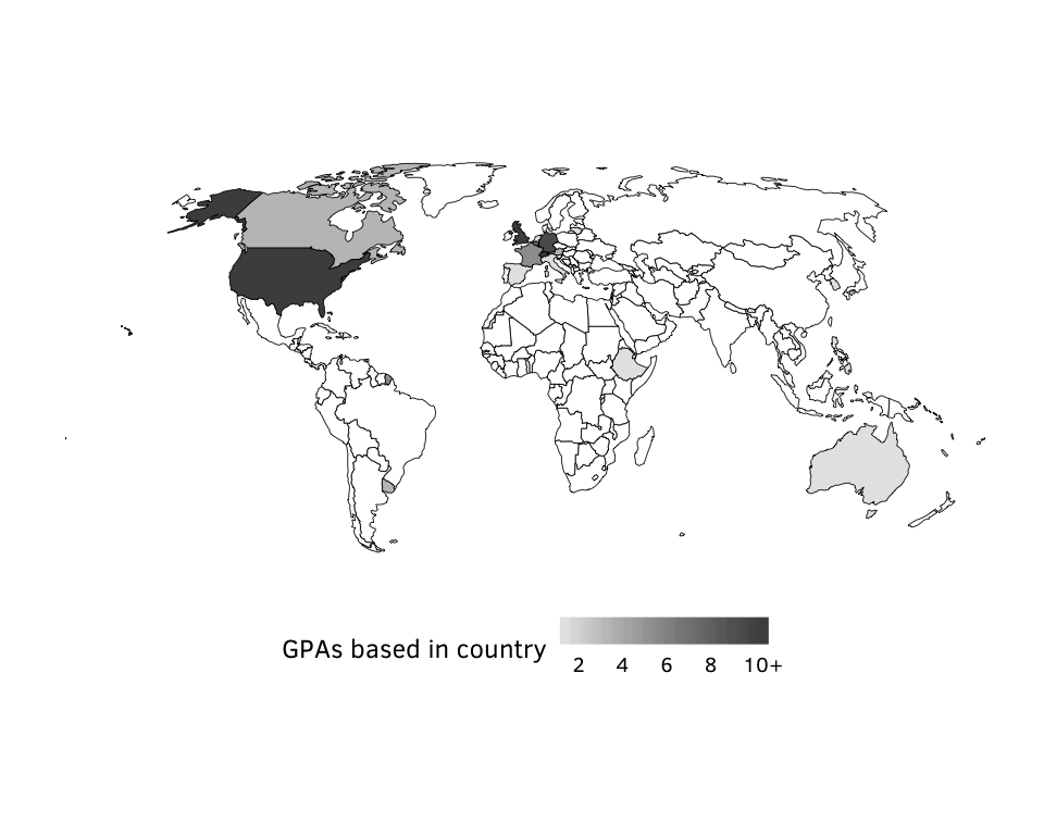
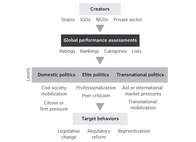
Figure 5: Pathways of GPA influence.
Source: Adapted from Kelley and Simmons, 2015.
(located at ./Output/figure-5-pathways.pdf and ./Output/figure-5-pathways.png)
Figure X: Pseudo-networks of indicator creators over time
Source: Authors’ data
gpa.data.clean.creator.long <- gpa.data.clean %>%
  separate_rows(subject_collapsed, sep=",") %>%
  mutate(subject_collapsed = str_trim(subject_collapsed))

subject.counts <- gpa.data.clean.creator.long %>%
  count(subject_collapsed) %>%
  arrange(desc(n))

gpa.creator.cumulative <- gpa.data.clean.creator.long %>%
  filter(!is.na(start_year)) %>%
  filter(!is.na(creator_collapsed)) %>%
  # Infer death year based on most recent year if not active
  mutate(end_year = ifelse(active == 0, recent_year, 2015)) %>%
  # Create list of years, like 1998:2005
  mutate(year = map2(start_year, end_year, ~ seq(.x, .y))) %>%
  # Unnest list of years
  unnest(year) %>%
  filter(year > 1970) %>%
  # Divide years into five-year chunks
  mutate(pentad = cut(year, breaks=seq(1970, 2015, 5), ordered_result=TRUE),
         pentad = fct_relabel(pentad, clean.cut.range)) %>%
  # Only select the first year in the pentad. Without this, indexes appear up
  # to five times in the pentad.
  filter(!is.na(pentad)) %>%
  group_by(pentad, gpa_id) %>%
  slice(1) %>%
  ungroup() %>%
  left_join(subject.counts, by="subject_collapsed") %>%
  arrange(pentad, desc(n)) %>%
  mutate(subject_collapsed = ordered(fct_inorder(subject_collapsed)),
         creator_collapsed = ordered(fct_relevel(creator_collapsed,
                                                 "NGO", "IGO", "State",
                                                 "University or Private",
                                                 "Other")))

# Export data
gpa.creator.cumulative %>%
  select(gpa_id, gpa_name, start_year, recent_year,
         subject = subject_collapsed, creator = creator_collapsed) %>%
  arrange(start_year) %>%
  write_csv(path = file.path(PROJHOME, "Output", "gpa_creator_cumulative.csv"))

# gpa.creator.cumulative %>%
#   count(pentad, subject_collapsed) %>%
#   spread(pentad, nn) %>%
#   write_csv("~/Desktop/gpa_subject_pentads.csv", na = "")
#
# gpa.creator.cumulative %>%
#   count(creator_collapsed, subject_collapsed) %>%
#   spread(creator_collapsed, nn) %>%
#   write_csv("~/Desktop/gpa_subject_creators.csv", na = "")
#
# gpa.creator.cumulative %>%
#   count(pentad, subject_collapsed, creator_collapsed) %>%
#   spread(pentad, nn) %>%
#   write_csv("~/Desktop/gpa_subject_creator_pentads.csv", na = "")
# position_jitternormal() comes from the development version of ggforce, which isn't on CRAN yet.
# Install from GitHub to use: devtools::install_github('thomasp85/ggforce')
gpa.type.points <- ggplot(gpa.creator.cumulative,
aes(x=pentad, y=subject_collapsed,
shape=creator_collapsed)) +
# geom_point(size=0.75, alpha=0.75, position=position_jitter(width=0.25, height=0.30)) +
geom_point(size=0.75, alpha=0.6, position=position_jitternormal(sd_x=0.1, sd_y=0.16)) +
labs(x=NULL, y=NULL) +
guides(shape=guide_legend(title=NULL, override.aes=list(size=3))) +
scale_shape_manual(values=c(16, 21, 17, 24, 3)) +
theme_gpa() +
theme(axis.text.x=element_text(angle=45, hjust=0.5, vjust=0.5),
panel.grid.major=element_blank())
set.seed(12345); gpa.type.points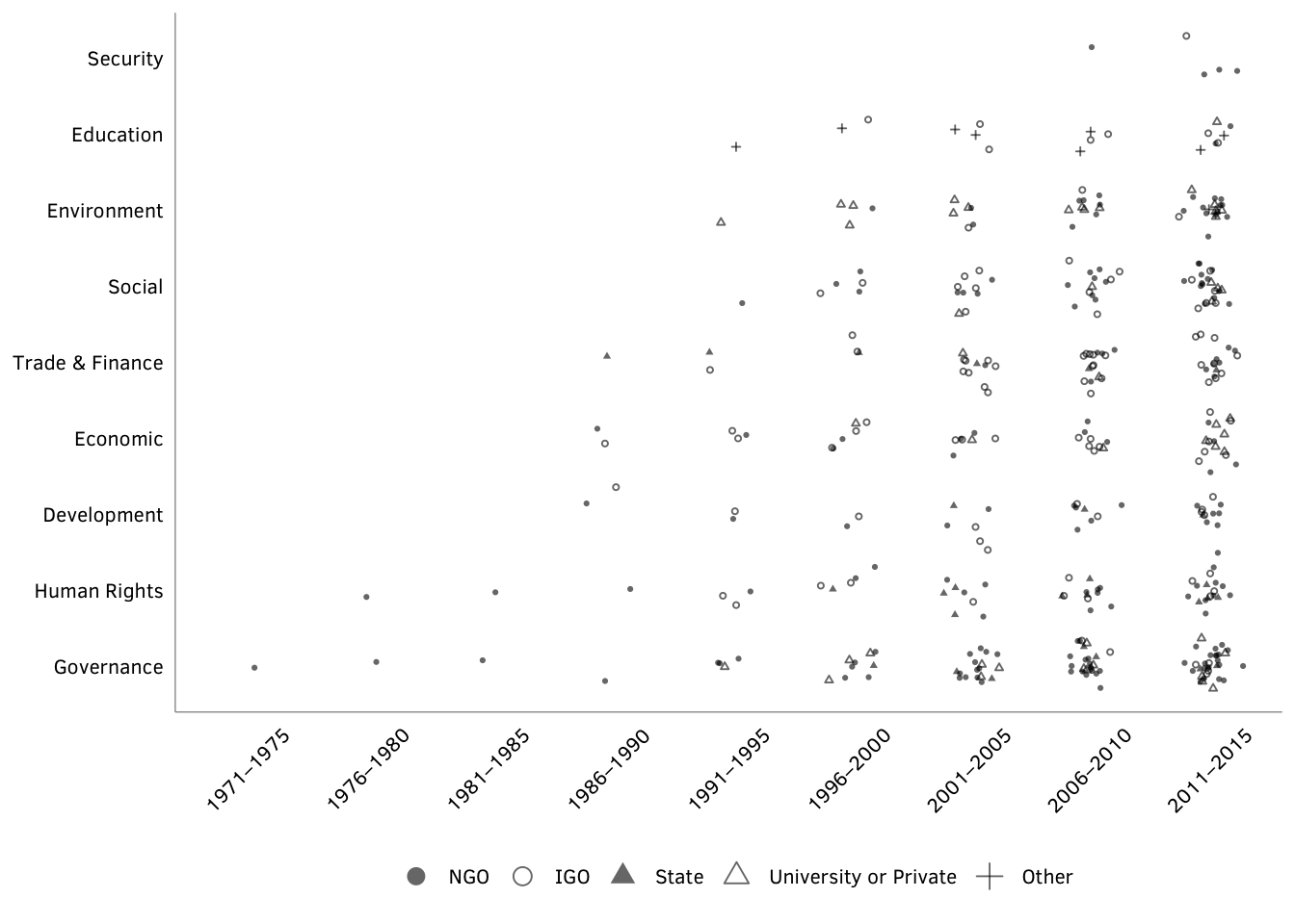
Figure X: Creator types over time
Source: Authors’ data
creator.types.time <- gpa.creator.cumulative %>%
  group_by(pentad, creator_collapsed, active) %>%
  summarize(n = n()) %>%
  filter(active == TRUE) %>%
  ungroup() %>%
  arrange(desc(n)) %>%
  mutate(creator_collapsed = str_replace(creator_collapsed, " or ", "\\\nor ")) %>%
  mutate(creator_collapsed = fct_inorder(creator_collapsed))

creator.types.labs <- creator.types.time %>%
  group_by(creator_collapsed) %>%
  slice(1)

creator.types.lines <- ggplot(creator.types.time,
                              aes(x = pentad, y = n,
                                  color = creator_collapsed,
                                  group = creator_collapsed)) +
  geom_line(size = 1) +
  geom_label(data = creator.types.labs, aes(x = pentad, y = n, label = creator_collapsed),
             hjust = 0, nudge_x = 0.1, size = 3) +
  labs(x=NULL, y=NULL) +
  scale_color_manual(values=c("black", "grey25", "grey45", "grey60", "grey70")) +
  expand_limits(x = 10.6, y = 80) +
  guides(color = FALSE) +
  theme_gpa() +
  theme(axis.text.x=element_text(angle=45, hjust=0.5, vjust=0.5),
        panel.grid.minor=element_blank())
creator.types.lines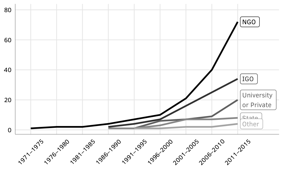
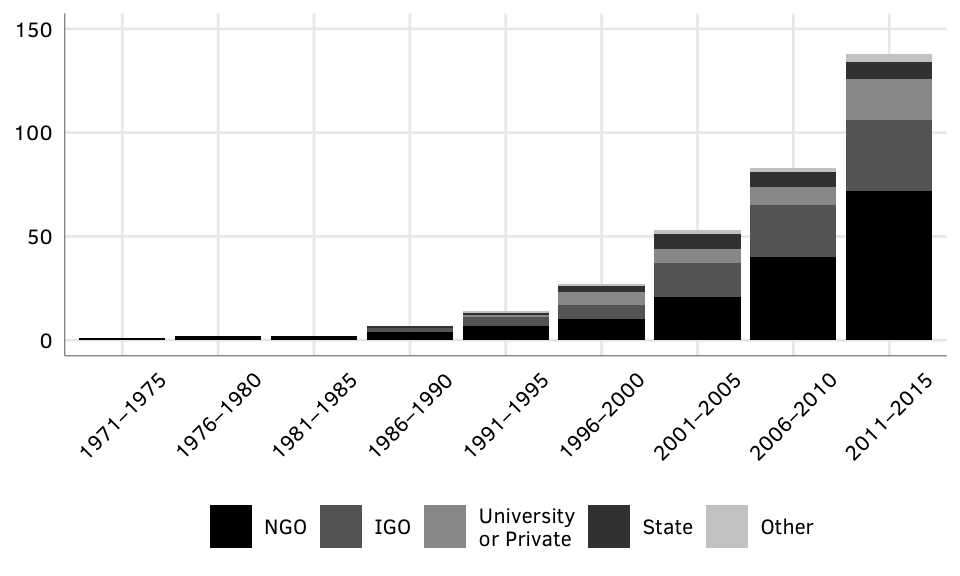
Figure X: Creator types over time
Source: Authors’ data
creator.types.bars <- ggplot(creator.types.time,
                             aes(x = pentad, y = n, fill = fct_rev(creator_collapsed))) +
  geom_bar(stat = "identity") +
  labs(x = NULL,  y = NULL) +
  expand_limits(y = 150) +
  scale_fill_manual(values=rev(c("black", "grey40", "grey60", "grey25", "grey80"))) +
  guides(fill=guide_legend(reverse=TRUE, title=NULL, nrow=1)) +
  theme_gpa() +
  theme(axis.text.x=element_text(angle=45, hjust=0.5, vjust=0.5),
        panel.grid.minor=element_blank())
creator.types.bars