Commitments to reform
Judith Kelley and Beth Simmons
March 10, 2017
library(tidyverse)
library(lubridate)
library(stringr)
library(forcats)
library(ggstance)
library(scales)
library(countrycode)
library(pander)
library(DT)

# Useful functions
theme_gpa <- function(base_size=10, base_family="Clear Sans") {
  update_geom_defaults("bar", list(fill = "grey30"))
  update_geom_defaults("line", list(colour = "grey30"))
  update_geom_defaults("label", list(family="Clear Sans"))
  update_geom_defaults("text", list(family="Clear Sans"))
  ret <- theme_bw(base_size, base_family) +
    theme(panel.background = element_rect(fill="#ffffff", colour=NA),
          axis.title.y = element_text(margin = margin(r = 10)),
          axis.title.x = element_text(margin = margin(t = 10)),
          axis.text = element_text(colour="black"),
          title=element_text(vjust=1.2, family="Clear Sans", face="bold"),
          plot.subtitle=element_text(family="Clear Sans"),
          plot.caption=element_text(family="Clear Sans",
                                    size=rel(0.8), colour="grey70"),
          panel.border = element_blank(),
          axis.line=element_line(colour="grey50", size=0.2),
          #panel.grid=element_blank(),
          axis.ticks=element_blank(),
          legend.position="bottom",
          legend.title=element_text(size=rel(0.8)),
          axis.title=element_text(size=rel(0.8), family="Clear Sans", face="bold"),
          strip.text=element_text(size=rel(1), family="Clear Sans", face="bold"),
          strip.background=element_rect(fill="#ffffff", colour=NA),
          panel.spacing.y=unit(1.5, "lines"),
          legend.key=element_blank(),
          legend.spacing=unit(0.2, "lines"))

  ret
}
Lexis Nexis query
We wanted to find all governemnt reactions to the EDB report in 2016. We used this big long Lexis Nexis query to identify all potential stories:
(("ease of doing business" W/50 (index OR report OR rank*) W/50 (fall* OR jump* OR improve* OR boost* OR high*) W/50 (minister OR secretary OR president OR MP OR PM)) and Date(geq(01/01/2016) and leq(12/31/2016)))We also enabled duplicate filtering (with moderate similarity). We then downloaded the results in 200-story chunks (the Lexis Nexis maximum) as plain text, including the fields BODY, GEOGRAPHIC, and LENGTH. We ran the Python script ln2csv.py in ./Data/ to clean each chunk and save them as a CSV file. Below we combine the chunks and do some additional cleaning.
Stories over time
There are definitely false positives in the results, but just to get the gist of the data, here’s what the distribution of stories looks like during 2016. There’s a clear peak in coverage in October, since that’s when the EDB report is released.
stories_2016 <- bind_rows(read_csv(file.path(PROJHOME, "Data",
                                             "2016-1.csv")),
                          read_csv(file.path(PROJHOME, "Data",
                                             "2016-2.csv")),
                          read_csv(file.path(PROJHOME, "Data",
                                             "2016-3.csv"))) %>%
  mutate(id = 1:n())
stories_timeline <- stories_2016 %>%
mutate(isoweek = format(DATE, format="%Y-W%V")) %>%
group_by(isoweek) %>%
summarise(num = n()) %>%
ungroup() %>%
mutate(date = parse_date_time(paste0(isoweek, "-1"), "YWw"))
ggplot(stories_timeline, aes(x=date, y=num)) +
geom_line() +
labs(x=NULL, y="Number of stories") +
scale_x_datetime(labels=date_format("%B %Y")) +
theme_gpa()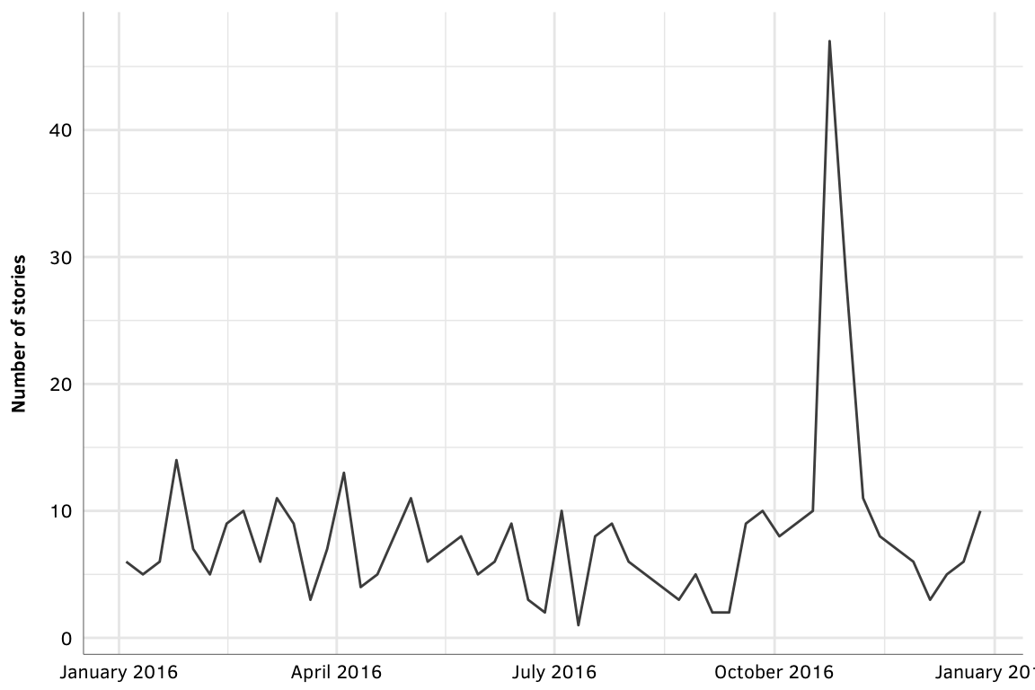
Reactions by country
Identifying the country for each of these stories is a little tricky. The GEOGRAPHIC column lists the countries and cities that Lexis Nexis’s algorithm determines the stories are about, along with a confidence percentage, like these:
AMMAN, JORDAN (90%) JORDAN (94%)ZIMBABWE (94%); UNITED STATES (79%); EUROPE (79%)
They’re not consistently delimited (except by %)), but even if they were, they’re not entirely perfect or accruate. Ideally, we could choose the top-scored location, but that’s not always right (and sometimes is something unhelpful like ASIA (98%)). So instead, we have to manually code each story. Boo.
Here’s the distribution of stories after manual coding. Again, there are a ton of false positives here—the US is the 4th most common country, but none of the stories really actually mention the EDB index. India seems to really, really, really care about the EDB.
to_code <- stories_2016 %>%
  separate_rows(GEOGRAPHIC, sep="%\\)") %>%
  # Extract the confidence value
  mutate(geo_confidence = str_match(GEOGRAPHIC, "\\((\\d+)")[,1],
         geo_confidence = str_replace(geo_confidence, "\\(", ""),
         GEOGRAPHIC = str_replace(GEOGRAPHIC, "\\(\\d+", "")) %>%
  # Sort by confidence level
  arrange(id, desc(geo_confidence)) %>%
  mutate(country = countrycode(GEOGRAPHIC, "country.name", "country.name"))

write_csv(to_code, file.path(PROJHOME, "Data",
                             "stories_to_code_WILL_BE_OVERWRITTEN.csv"))
coded_stories <- read_csv(file.path(PROJHOME, "Data", "coded_stories_2016.csv"))
country_reactions <- stories_2016 %>%
left_join(coded_stories, by="id") %>%
group_by(country_fixed) %>%
summarise(num = n()) %>%
ungroup() %>%
arrange(num) %>%
mutate(country_fixed = fct_inorder(country_fixed, ordered=TRUE))
ggplot(country_reactions, aes(x=num, y=country_fixed)) +
geom_barh(stat="identity") +
labs(x="Number of stories", y=NULL) +
theme_gpa()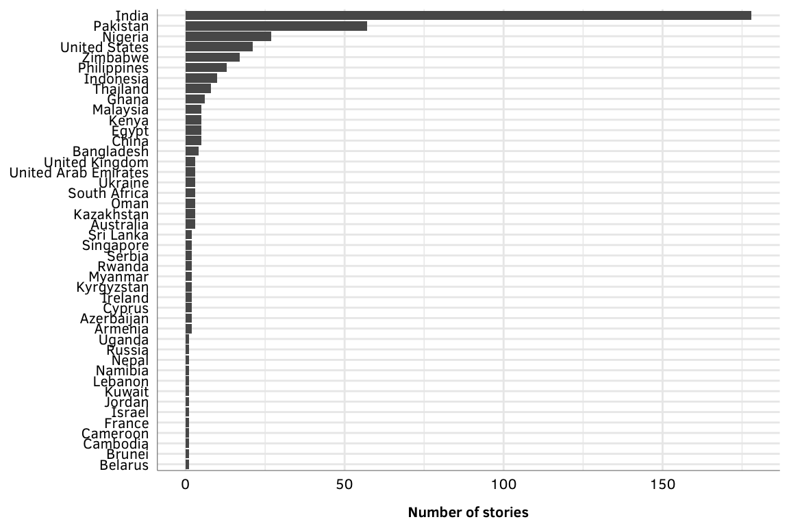
Actual stories
Lots of these stories are either false positives or don’t directly mention government reactions to the report. We looked at each story manually and identified quotes or statements made by official people. This is saved in ./Data/quotes_clean.csv and also included in the table below (click on the plus sign to see the full quote if it’s not visible).
reactions_for_coding <- stories_2016 %>%
  left_join(coded_stories, by="id") %>%
  select(id, country_fixed, DATE, HEADLINE, BODY)

# reactions_for_coding %>%
#   split(.$country_fixed) %>%
#   map(~ pandoc.table(., split.cells=Inf, split.tables=Inf))
quotes.raw <- read_csv(file.path(PROJHOME, "Data", "quotes.csv")) %>%
select(-country_fixed)
quotes <- quotes.raw %>%
left_join(coded_stories, by="id") %>%
left_join(stories_2016, by="id") %>%
select(id, country = country_fixed, person, position, quote, date=DATE,
publication = PUBLICATION, headline = HEADLINE) %>%
arrange(country, date)
write_excel_csv(quotes, file.path(PROJHOME, "Data", "quotes_clean.csv"), na="")quotes %>% datatable(extensions = "Responsive")