Determinants of international civil society restrictions
Andrew Heiss
August 9, 2016
Load libraries and data
library(magrittr)
library(dplyr)
library(purrr)
library(broom)
library(feather)
library(ggplot2)
library(scales)
library(gridExtra)
library(Cairo)
library(stargazer)

source(file.path(PROJHOME, "Analysis", "lib", "graphic_functions.R"))

full.data <- read_feather(file.path(PROJHOME, "Data", "data_processed",
                               "full_data.feather"))

my.seed <- 1234
set.seed(my.seed)
Variables
Dependent variables
Civil society regulatory environment:
v2csreprss: V-Dem CSO repression (“Does the government attempt to repress civil society organizations?). Higher numbers = less repression.v2csreprss_ord: Ordinal version ofv2csreprss(labels = “Severely”, “Substantially”, “Moderately”, “Weakly”, “No”)v2cseeorgs: V-Dem CSO entry and exit (“To what extent does the government achieve control over entry and exit by civil society organizations (CSOs) into public life?”). Higher numbers = less control.cs_env_sum: Sum ofv2csreprssandv2cseeorgs. V-Dem includes a “Core civil society index” that uses Bayesian factor analysis to combine repression, entry/exit, and participatory environment. I’m less interested in the participatory environment. The paper describing the original factor analysis model, however, does not explain how it was built, so here I make a simple additive index of the two variables.
Explanatory variables
Internal stability:
icrg.stability:icrg.pol.risk.internal.scaled: Political risk rating—external measures removed and index rescaled to 0-100 scaleyrsoffc:years.since.comp:opp1vote:
External stability:
neighbor.pol.risk.XXX
International reputation:
- Variable from ICEWS / shaming data from Murdie
Controls:
e_polity2:physint:gdpcap.log:population.log:oda.log:countngo:globalization:
Preliminary large-N analysis (LNA)
There are lots of different ways to define autocracy, including Polity, UDS, or Geddes et al.’s manual classification. Here, I follow Geddes et al., but slightly expanded—for the sake of completeness of data (and in case I run survival models in the future), I include a country in the data if it has ever been an autocracy since 1991. This means countries that democratize or backslide are included.
autocracies <- filter(full.data, gwf.ever.autocracy) %>%
  mutate(case.study = cowcode %in% c(710, 651, 365)) %>%
  # Make these variables more interpretable unit-wise
  mutate_each(funs(. * 100), dplyr::contains("pct")) %>%
  mutate(.rownames = rownames(.))
Note on time frame of variables: Not all variables overlap perfectly with V-Dem. Models that include any of the following variables will be inherently limited to the corresponding years (since non-overlapping years are dropped):
- ICRG: 1991-2014
- ICEWS: 1995-2015
- ICEWS EOIs: 2000-2014
All models
lna.all.simple <- lm(cs_env_sum.lead ~
                       icrg.stability + icrg.internal +
                       icrg.pol.risk_wt +
                       shaming.states.std +
                       shaming.ingos.std +
                       as.factor(year.num),
                     data=autocracies)

lna.all.full <- lm(cs_env_sum.lead ~
                     # Internal
                     icrg.stability + icrg.internal +
                     yrsoffc + years.since.comp + opp1vote +
                     # External
                     # any.crisis_pct_wt +
                     # insurgency_pct_mean_nb +
                     icrg.pol.risk_wt +
                     any.crisis_pct_mean_nb +
                     coups.activity.bin_sum_nb +
                     protests.violent.std_wt +
                     protests.nonviolent.std_wt +
                     # Shaming
                     shaming.states.std +
                     shaming.ingos.std +
                     # Minimal controls
                     as.factor(year.num),
                   data=autocracies)
Internal factors
Models
lna.internal.simple <- lm(cs_env_sum.lead ~
                            # Internal (low is bad; high is good)
                            icrg.stability + icrg.internal +
                            as.factor(year.num),
                          data=autocracies)

lna.internal.full <- lm(cs_env_sum.lead ~
                          icrg.stability + icrg.internal +
                          yrsoffc + years.since.comp + opp1vote +
                          as.factor(year.num),
                        data=autocracies)

lna.internal.alt <- lm(cs_env_sum.lead ~
                         icrg.pol.risk.internal.scaled +
                         yrsoffc + years.since.comp + opp1vote +
                         as.factor(year.num),
data=autocracies)stargazer(lna.internal.simple, lna.internal.full,
lna.all.simple, lna.all.full,
type="html",
dep.var.caption="CSRE in following year",
dep.var.labels.include=FALSE, no.space=TRUE,
omit="\\.factor",
add.lines=list(c("Year fixed effects",
rep("Yes", 4))))| CSRE in following year | ||||
| (1) | (2) | (3) | (4) | |
| icrg.stability | -0.339*** | -0.234*** | -0.567*** | -0.201** |
| (0.049) | (0.050) | (0.069) | (0.081) | |
| icrg.internal | 0.176*** | 0.234*** | 0.115** | 0.081 |
| (0.034) | (0.035) | (0.050) | (0.070) | |
| yrsoffc | -0.084*** | -0.102*** | ||
| (0.009) | (0.013) | |||
| years.since.comp | -0.052*** | -0.033*** | ||
| (0.007) | (0.009) | |||
| opp1vote | 0.041*** | 0.041*** | ||
| (0.005) | (0.009) | |||
| icrg.pol.risk_wt | -0.005 | -0.060*** | ||
| (0.011) | (0.016) | |||
| any.crisis_pct_mean_nb | -0.018*** | |||
| (0.005) | ||||
| coups.activity.bin_sum_nb | 0.598** | |||
| (0.265) | ||||
| protests.violent.std_wt | -0.282 | |||
| (0.204) | ||||
| protests.nonviolent.std_wt | 0.652*** | |||
| (0.200) | ||||
| shaming.states.std | -0.163* | 0.170* | ||
| (0.091) | (0.102) | |||
| shaming.ingos.std | -0.191** | -0.062 | ||
| (0.093) | (0.096) | |||
| Constant | 1.133*** | 1.505*** | 3.257*** | 5.854*** |
| (0.400) | (0.403) | (0.872) | (1.308) | |
| Year fixed effects | Yes | Yes | Yes | Yes |
| Observations | 1,520 | 875 | 877 | 335 |
| R2 | 0.048 | 0.420 | 0.092 | 0.539 |
| Adjusted R2 | 0.033 | 0.402 | 0.066 | 0.505 |
| Residual Std. Error | 2.538 (df = 1494) | 1.967 (df = 848) | 2.595 (df = 852) | 1.809 (df = 311) |
| F Statistic | 3.044*** (df = 25; 1494) | 23.584*** (df = 26; 848) | 3.584*** (df = 24; 852) | 15.837*** (df = 23; 311) |
| Note: | p<0.1; p<0.05; p<0.01 | |||
Coefficient plot
vars.included <- c("icrg.stability", "icrg.internal", "yrsoffc",
                   "years.since.comp", "opp1vote")

coef.plot.int <- fig.coef(list("Simple" = lna.internal.simple,
                               "All internal factors" = lna.internal.full,
                               "All factors (excerpt)" = lna.all.full),
                          xlab="Civil society regulatory environment (CSRE)",
                          vars.included=vars.included)
coef.plot.int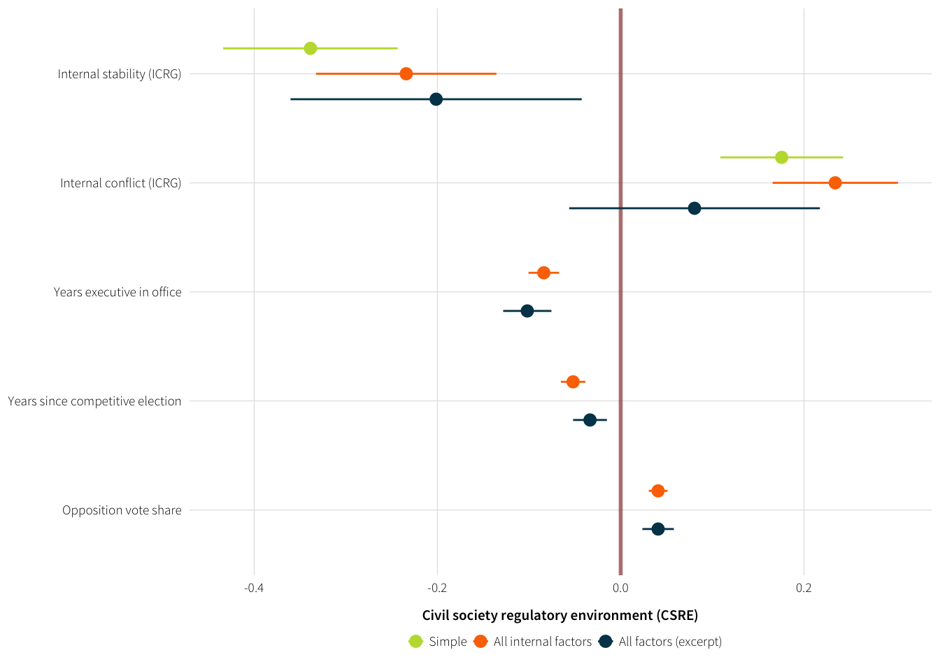
fig.save.cairo(coef.plot.int, filename="1-coefs-lna-int",
               width=6, height=3)
External factors
Models
lna.external.simple <- lm(cs_env_sum.lead ~
                             icrg.pol.risk_wt +
                            as.factor(year.num),
                          data=autocracies)

lna.external.full <- lm(cs_env_sum.lead ~
                          # TODO: Consistent wt vs nb variables? Or
                          # justification for them being different?
                          icrg.pol.risk_wt +
                          any.crisis_pct_mean_nb +
                          coups.activity.bin_sum_nb +
                          protests.violent.std_wt +
                          protests.nonviolent.std_wt +
                          as.factor(year.num),
data=autocracies)stargazer(lna.external.simple, lna.external.full,
lna.all.simple, lna.all.full,
type="html",
dep.var.caption="CSRE in following year",
dep.var.labels.include=FALSE, no.space=TRUE,
omit="\\.factor",
add.lines=list(c("Year fixed effects",
rep("Yes", 4))))| CSRE in following year | ||||
| (1) | (2) | (3) | (4) | |
| icrg.stability | -0.567*** | -0.201** | ||
| (0.069) | (0.081) | |||
| icrg.internal | 0.115** | 0.081 | ||
| (0.050) | (0.070) | |||
| yrsoffc | -0.102*** | |||
| (0.013) | ||||
| years.since.comp | -0.033*** | |||
| (0.009) | ||||
| opp1vote | 0.041*** | |||
| (0.009) | ||||
| icrg.pol.risk_wt | -0.012* | -0.040*** | -0.005 | -0.060*** |
| (0.007) | (0.011) | (0.011) | (0.016) | |
| shaming.states.std | -0.163* | 0.170* | ||
| (0.091) | (0.102) | |||
| shaming.ingos.std | -0.191** | -0.062 | ||
| (0.093) | (0.096) | |||
| any.crisis_pct_mean_nb | -0.039*** | -0.018*** | ||
| (0.004) | (0.005) | |||
| coups.activity.bin_sum_nb | 0.605*** | 0.598** | ||
| (0.200) | (0.265) | |||
| protests.violent.std_wt | -0.245* | -0.282 | ||
| (0.139) | (0.204) | |||
| protests.nonviolent.std_wt | 0.447*** | 0.652*** | ||
| (0.139) | (0.200) | |||
| Constant | 0.821* | 4.569*** | 3.257*** | 5.854*** |
| (0.458) | (0.806) | (0.872) | (1.308) | |
| Year fixed effects | Yes | Yes | Yes | Yes |
| Observations | 1,942 | 1,094 | 877 | 335 |
| R2 | 0.013 | 0.114 | 0.092 | 0.539 |
| Adjusted R2 | 0.0004 | 0.099 | 0.066 | 0.505 |
| Residual Std. Error | 2.619 (df = 1917) | 2.507 (df = 1075) | 2.595 (df = 852) | 1.809 (df = 311) |
| F Statistic | 1.035 (df = 24; 1917) | 7.661*** (df = 18; 1075) | 3.584*** (df = 24; 852) | 15.837*** (df = 23; 311) |
| Note: | p<0.1; p<0.05; p<0.01 | |||
Coefficient plot
vars.included <- c("icrg.pol.risk_wt", "any.crisis_pct_mean_nb",
                   "coups.activity.bin_sum_nb", "protests.violent.std_wt",
                   "protests.nonviolent.std_wt")

coef.plot.ext <- fig.coef(list("Simple" = lna.external.simple,
                               "All external factors" = lna.external.full,
                               "All factors (excerpt)" = lna.all.full),
                          xlab="Civil society regulatory environment (CSRE)",
                          vars.included=vars.included)
coef.plot.ext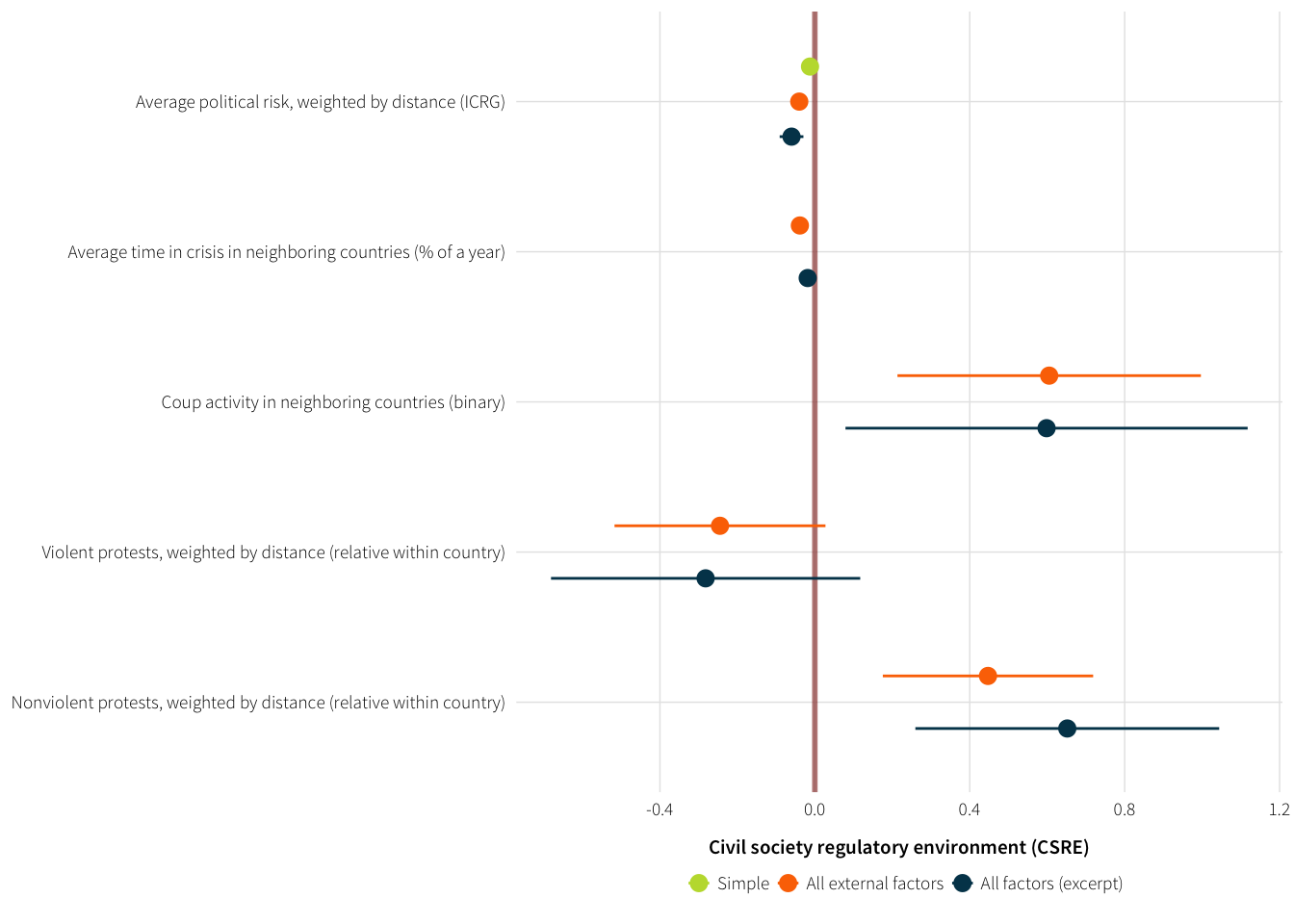
fig.save.cairo(coef.plot.ext, filename="1-coefs-lna-ext",
               width=6, height=3)
Shaming factors
Models
lna.shame.simple <- lm(cs_env_sum.lead ~
                         # TODO: Deal with proper normalized or weighted values
                         # shaming.states.pct.govt +
                         # shaming.ingos.pct.ingo +
                         shaming.states.std +
                         shaming.ingos.std +
                         as.factor(year.num),
data=autocracies)stargazer(lna.shame.simple, lna.all.simple, lna.all.full,
type="html",
dep.var.caption="CSRE in following year",
dep.var.labels.include=FALSE, no.space=TRUE,
omit="\\.factor",
add.lines=list(c("Year fixed effects",
rep("Yes", 3))))| CSRE in following year | |||
| (1) | (2) | (3) | |
| icrg.stability | -0.567*** | -0.201** | |
| (0.069) | (0.081) | ||
| icrg.internal | 0.115** | 0.081 | |
| (0.050) | (0.070) | ||
| yrsoffc | -0.102*** | ||
| (0.013) | |||
| years.since.comp | -0.033*** | ||
| (0.009) | |||
| opp1vote | 0.041*** | ||
| (0.009) | |||
| icrg.pol.risk_wt | -0.005 | -0.060*** | |
| (0.011) | (0.016) | ||
| any.crisis_pct_mean_nb | -0.018*** | ||
| (0.005) | |||
| coups.activity.bin_sum_nb | 0.598** | ||
| (0.265) | |||
| protests.violent.std_wt | -0.282 | ||
| (0.204) | |||
| protests.nonviolent.std_wt | 0.652*** | ||
| (0.200) | |||
| shaming.states.std | -0.176** | -0.163* | 0.170* |
| (0.086) | (0.091) | (0.102) | |
| shaming.ingos.std | -0.089 | -0.191** | -0.062 |
| (0.088) | (0.093) | (0.096) | |
| Constant | 0.322 | 3.257*** | 5.854*** |
| (0.385) | (0.872) | (1.308) | |
| Year fixed effects | Yes | Yes | Yes |
| Observations | 1,076 | 877 | 335 |
| R2 | 0.015 | 0.092 | 0.539 |
| Adjusted R2 | -0.005 | 0.066 | 0.505 |
| Residual Std. Error | 2.722 (df = 1054) | 2.595 (df = 852) | 1.809 (df = 311) |
| F Statistic | 0.768 (df = 21; 1054) | 3.584*** (df = 24; 852) | 15.837*** (df = 23; 311) |
| Note: | p<0.1; p<0.05; p<0.01 | ||
Coefficient plot
vars.included <- c("shaming.states.std", "shaming.ingos.std")
coef.plot.shame <- fig.coef(list("All shaming factors" = lna.shame.simple,
                                 "All factors (excerpt)" = lna.all.full),
                            xlab="Civil society regulatory environment (CSRE)",
                            vars.included=vars.included)
coef.plot.shame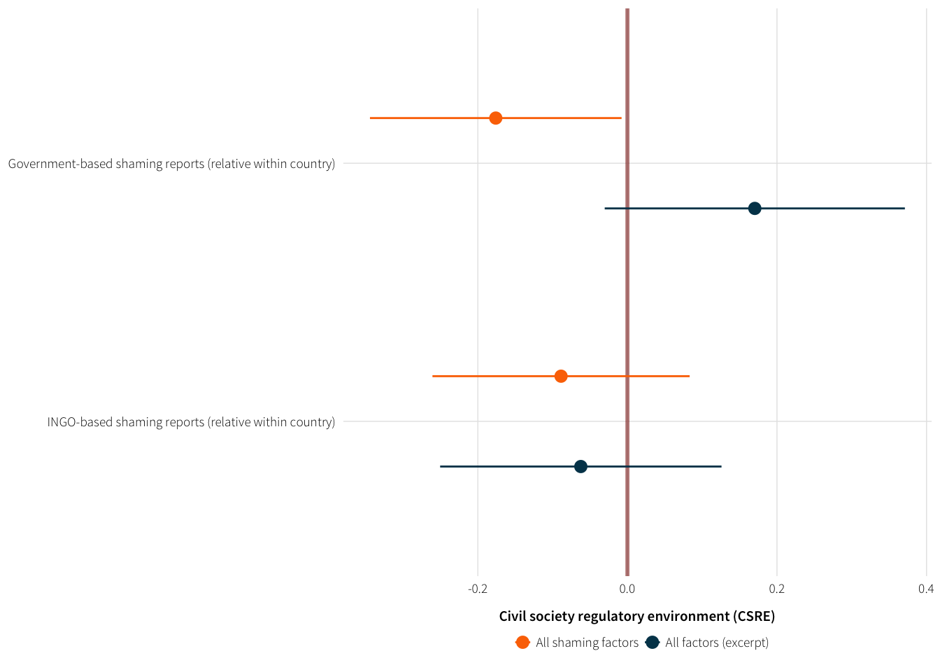
fig.save.cairo(coef.plot.shame, filename="1-coefs-lna-shame",
               width=6, height=3)
All factors at once
Models
Actual full models run previously so they can be compared to smaller models.
Here I show the results of all models side-by-side.
var.labs <-  c(
  "Internal stability (ICRG)",
  "Internal conflict (ICRG)",
  "Years executive in office",
  "Years since competitive election",
  "Opposition vote share",
  "Average political risk in neighboring countries (ICRG)",
  "Government-based shaming reports (% of all events)",
  "INGO-based shaming reports (% of all events)",
  "Average time in crisis in neighboring countries (% of a year)",
  "Coup activity in neighboring countries (binary)",
  "Violent protests, weighted by distance (relative within country)",
  "Nonviolent protests, weighted by distance (relative within country)"
)stargazer(lna.internal.simple, lna.internal.full,
lna.external.simple, lna.external.full,
lna.shame.simple, lna.all.simple, lna.all.full,
type="html",
dep.var.caption="CSRE in following year",
dep.var.labels.include=FALSE, no.space=TRUE,
# covariate.labels=var.labs,
omit="\\.factor",
add.lines=list(c("Year fixed effects",
rep("Yes", 7)))#,
# out=file.path("~/Desktop/all.html")
)| CSRE in following year | |||||||
| (1) | (2) | (3) | (4) | (5) | (6) | (7) | |
| icrg.stability | -0.339*** | -0.234*** | -0.567*** | -0.201** | |||
| (0.049) | (0.050) | (0.069) | (0.081) | ||||
| icrg.internal | 0.176*** | 0.234*** | 0.115** | 0.081 | |||
| (0.034) | (0.035) | (0.050) | (0.070) | ||||
| yrsoffc | -0.084*** | -0.102*** | |||||
| (0.009) | (0.013) | ||||||
| years.since.comp | -0.052*** | -0.033*** | |||||
| (0.007) | (0.009) | ||||||
| opp1vote | 0.041*** | 0.041*** | |||||
| (0.005) | (0.009) | ||||||
| icrg.pol.risk_wt | -0.012* | -0.040*** | -0.005 | -0.060*** | |||
| (0.007) | (0.011) | (0.011) | (0.016) | ||||
| shaming.states.std | -0.176** | -0.163* | 0.170* | ||||
| (0.086) | (0.091) | (0.102) | |||||
| shaming.ingos.std | -0.089 | -0.191** | -0.062 | ||||
| (0.088) | (0.093) | (0.096) | |||||
| any.crisis_pct_mean_nb | -0.039*** | -0.018*** | |||||
| (0.004) | (0.005) | ||||||
| coups.activity.bin_sum_nb | 0.605*** | 0.598** | |||||
| (0.200) | (0.265) | ||||||
| protests.violent.std_wt | -0.245* | -0.282 | |||||
| (0.139) | (0.204) | ||||||
| protests.nonviolent.std_wt | 0.447*** | 0.652*** | |||||
| (0.139) | (0.200) | ||||||
| Constant | 1.133*** | 1.505*** | 0.821* | 4.569*** | 0.322 | 3.257*** | 5.854*** |
| (0.400) | (0.403) | (0.458) | (0.806) | (0.385) | (0.872) | (1.308) | |
| Year fixed effects | Yes | Yes | Yes | Yes | Yes | Yes | Yes |
| Observations | 1,520 | 875 | 1,942 | 1,094 | 1,076 | 877 | 335 |
| R2 | 0.048 | 0.420 | 0.013 | 0.114 | 0.015 | 0.092 | 0.539 |
| Adjusted R2 | 0.033 | 0.402 | 0.0004 | 0.099 | -0.005 | 0.066 | 0.505 |
| Residual Std. Error | 2.538 (df = 1494) | 1.967 (df = 848) | 2.619 (df = 1917) | 2.507 (df = 1075) | 2.722 (df = 1054) | 2.595 (df = 852) | 1.809 (df = 311) |
| F Statistic | 3.044*** (df = 25; 1494) | 23.584*** (df = 26; 848) | 1.035 (df = 24; 1917) | 7.661*** (df = 18; 1075) | 0.768 (df = 21; 1054) | 3.584*** (df = 24; 852) | 15.837*** (df = 23; 311) |
| Note: | p<0.1; p<0.05; p<0.01 | ||||||
Coefficient plot
coef.plot.all <- fig.coef(list("Simple" = lna.all.simple,
                               "Full" = lna.all.full),
                          xlab="Civil society regulatory environment (CSRE)")
coef.plot.all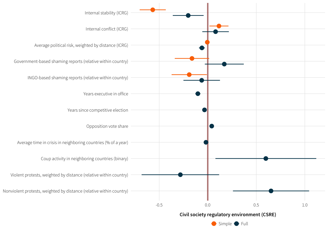
fig.save.cairo(coef.plot.all, filename="1-coefs-lna-all",
               width=6, height=4.5)

# ggplot(autocracies, aes(x=shaming.ingos.pct.all, y=cs_env_sum.lead)) +
#   geom_point(aes(text=paste(country_name, year.num), colour=case.study)) +
#   geom_smooth() #+ facet_wrap(~ case.study)
# plotly::ggplotly()
Marginal effects
CSRE across internal variables
new.data.int.stability <- lna.internal.full$model %>%
  summarise_each(funs(mean), -c(`as.factor(year.num)`)) %>%
  mutate(year.num = 2005,
         index = 1) %>%
  select(-c(cs_env_sum.lead, icrg.stability, yrsoffc)) %>%
  right_join(expand.grid(icrg.stability =
                           seq(0, 12, by=0.1),
                         yrsoffc = c(2, 30),
                         index = 1),
             by="index") %>%
  select(-index)

new.data.int.conflict <- lna.internal.full$model %>%
  summarise_each(funs(mean), -c(`as.factor(year.num)`)) %>%
  mutate(year.num = 2005,
         index = 1) %>%
  select(-c(cs_env_sum.lead, icrg.internal, yrsoffc)) %>%
  right_join(expand.grid(icrg.internal =
                           seq(0, 12, by=0.1),
                         yrsoffc = c(2, 30),
                         index = 1),
             by="index") %>%
  select(-index)

plot.predict.stability <- lna.internal.full %>%
  augment(newdata=new.data.int.stability) %>%
  mutate(val.to.plot = icrg.stability,
         var.name = "Internal stability")

plot.predict.conflict <- lna.internal.full %>%
  augment(newdata=new.data.int.conflict) %>%
  mutate(val.to.plot = icrg.internal,
         var.name = "Internal conflict")

plot.predict <- bind_rows(plot.predict.stability, plot.predict.conflict) %>%
  mutate(pred = .fitted,
         pred.lower = pred + (qnorm(0.025) * .se.fit),
         pred.upper = pred + (qnorm(0.975) * .se.fit)) %>%
  mutate(yrsoffc = factor(yrsoffc, levels=c(2, 30),
                          labels=paste(c(2, 30), "years in office")))

plot.icrg.int.pred <- ggplot(plot.predict,
                             aes(x=val.to.plot, y=pred,
                                 fill=var.name, colour=var.name)) +
  geom_ribbon(aes(ymin=pred.lower, ymax=pred.upper),
              alpha=0.3, colour=NA) +
  geom_line(size=1.5) +
  labs(x="ICRG score", y="Predicted CSRE in following year") +
  scale_colour_manual(values=c(col.auth, col.dem), name=NULL) +
  scale_fill_manual(values=c(col.auth, col.dem), name=NULL, guide=FALSE) +
  coord_cartesian(ylim=c(-4, 4)) +
  theme_ath() +
  facet_wrap(~ yrsoffc)
plot.icrg.int.pred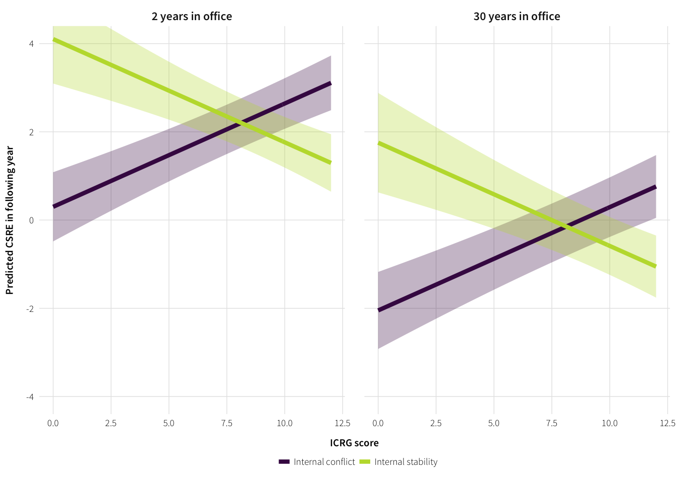
fig.save.cairo(plot.icrg.int.pred, filename="1-icrg-int-pred",
               width=5, height=3)
CSRE across external variables
new.data.ext <- lna.external.full$model %>%
  summarise_each(funs(mean), -c(`as.factor(year.num)`)) %>%
  mutate(year.num = 2005,
         index = 1) %>%
  select(-c(cs_env_sum.lead, protests.nonviolent.std_wt,
            icrg.pol.risk_wt)) %>%
  right_join(expand.grid(protests.nonviolent.std_wt = c(1, 2.5, 5),
                         icrg.pol.risk_wt = seq(40, 100, by=1),
                         index=1),
             by="index") %>%
  select(-index)

plot.predict.ext.icrg.protests <- lna.external.full %>%
  augment(newdata=new.data.ext) %>%
  mutate(pred = .fitted,
         pred.lower = pred + (qnorm(0.025) * .se.fit),
         pred.upper = pred + (qnorm(0.975) * .se.fit),
         protests = factor(protests.nonviolent.std_wt, levels=c(1, 2.5, 5),
                           labels=c("Much fewer than normal (1)", "Normal (2.5)",
                                    "Much more than normal (5)"))) %>%
  # Remove confidence intervals for normal levels of protests
  mutate(pred.lower = ifelse(protests.nonviolent.std_wt == 2.5, NA, pred.lower),
         pred.upper = ifelse(protests.nonviolent.std_wt == 2.5, NA, pred.upper))

plot.ext.icrg.nonviolent <- ggplot(plot.predict.ext.icrg.protests,
                                   aes(x=icrg.pol.risk_wt, y=pred,
                                       colour=protests)) +
  geom_ribbon(aes(ymin=pred.lower, ymax=pred.upper, fill=protests),
              alpha=0.3, colour=NA) +
  geom_line(size=1.5) +
  labs(x="Average political risk in neighboring countries (ICRG)",
       y="Predicted CSRE in following year") +
  scale_colour_manual(values=c("#004259", "grey50", "#4A0A3D"), name=NULL) +
  scale_fill_manual(values=c("#004259", "grey50" ,"#4A0A3D"), name=NULL, guide=FALSE) +
  theme_ath()
plot.ext.icrg.nonviolent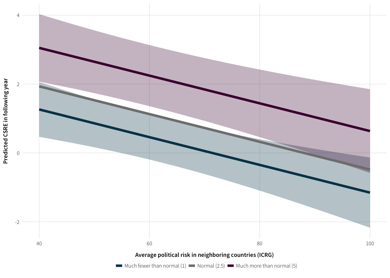
# fig.save.cairo(plot.subregion.coup.pred, filename="1-icrg-subregion-coup-ext-pred",
#                width=5, height=2.5)
#
CSRE across shaming variables
new.data.shame.states <- lna.all.full$model %>%
  summarise_each(funs(mean), -c(`as.factor(year.num)`)) %>%
  mutate(year.num = 2005,
         index = 1) %>%
  select(-c(cs_env_sum.lead, shaming.states.std)) %>%
  right_join(expand.grid(shaming.states.std =
                           seq(1, 5, by=0.1),
                         index = 1),
             by="index") %>%
  select(-index)

new.data.shame.ingos <- lna.all.full$model %>%
  summarise_each(funs(mean), -c(`as.factor(year.num)`)) %>%
  mutate(year.num = 2005,
         index = 1) %>%
  select(-c(cs_env_sum.lead, shaming.ingos.std)) %>%
  right_join(expand.grid(shaming.ingos.std =
                           seq(1, 5, by=0.1),
                         index = 1),
             by="index") %>%
  select(-index)

plot.predict.states <- lna.all.full %>%
  augment(newdata=new.data.shame.states) %>%
  mutate(val.to.plot = shaming.states.std,
         var.name = "State-based shaming")

plot.predict.ingos <- lna.all.full %>%
  augment(newdata=new.data.shame.ingos) %>%
  mutate(val.to.plot = shaming.ingos.std,
         var.name = "INGO-based shaming")

plot.predict.shame <- bind_rows(plot.predict.states, plot.predict.ingos) %>%
  mutate(pred = .fitted,
         pred.lower = pred + (qnorm(0.025) * .se.fit),
         pred.upper = pred + (qnorm(0.975) * .se.fit))

plot.shame.states.ingos <- ggplot(plot.predict.shame,
                                  aes(x=val.to.plot, y=pred,
                                      fill=var.name, colour=var.name)) +
  geom_ribbon(aes(ymin=pred.lower, ymax=pred.upper),
              alpha=0.3, colour=NA) +
  geom_line(size=1.5) +
  labs(x="Level of shaming", y="Predicted CSRE in following year") +
  scale_colour_manual(values=c(col.auth, col.dem), name=NULL) +
  scale_fill_manual(values=c(col.auth, col.dem), name=NULL, guide=FALSE) +
  coord_cartesian(ylim=c(-2, 4)) +
  theme_ath()
plot.shame.states.ingos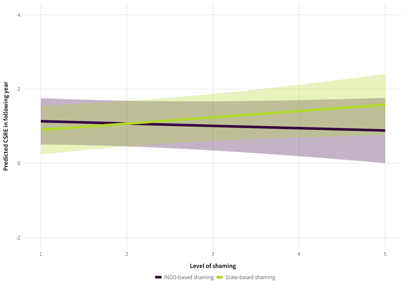
fig.save.cairo(plot.shame.states.ingos, filename="1-shame-states-ingos",
               width=5, height=3)
Robustness checks
Different external variables
robust.ext.no.eois <- lm(cs_env_sum.lead ~
                           icrg.pol.risk_wt +
                           coups.activity.bin_sum_nb +
                           protests.violent.std_wt +
                           protests.nonviolent.std_wt +
                           as.factor(year.num),
                         data=autocracies)

robust.ext.risk.nb <- lm(cs_env_sum.lead ~
                           icrg.pol.risk_mean_nb +
                           any.crisis_pct_mean_nb +
                           coups.activity.bin_sum_nb +
                           protests.violent.std_wt +
                           protests.nonviolent.std_wt +
                           as.factor(year.num),
                         data=autocracies)

robust.ext.risk.nb.no.eois <- lm(cs_env_sum.lead ~
                                   icrg.pol.risk_mean_nb +
                                   coups.activity.bin_sum_nb +
                                   protests.violent.std_wt +
                                   protests.nonviolent.std_wt +
                                   as.factor(year.num),
                                 data=autocracies)

robust.ext.protests.prop.wt <- lm(cs_env_sum.lead ~
                                    icrg.pol.risk_wt +
                                    any.crisis_pct_mean_nb +
                                    coups.activity.bin_sum_nb +
                                    protests.violent.pct.all_wt +
                                    protests.nonviolent.pct.all_wt +
                                    as.factor(year.num),
                                  data=autocracies)

robust.ext.protests.prop.nb <- lm(cs_env_sum.lead ~
                                    icrg.pol.risk_wt +
                                    any.crisis_pct_mean_nb +
                                    coups.activity.bin_sum_nb +
                                    protests.violent.pct.all_mean_nb +
                                    protests.nonviolent.pct.all_mean_nb +
                                    as.factor(year.num),
                                  data=autocracies)

robust.ext.protests.prop.wt.no.eois <- lm(cs_env_sum.lead ~
                                            icrg.pol.risk_wt +
                                            coups.activity.bin_sum_nb +
                                            protests.violent.pct.all_wt +
                                            protests.nonviolent.pct.all_wt +
                                            as.factor(year.num),
                                          data=autocracies)

robust.ext.protests.prop.nb.no.eois <- lm(cs_env_sum.lead ~
                                            icrg.pol.risk_wt +
                                            coups.activity.bin_sum_nb +
                                            protests.violent.pct.all_mean_nb +
                                            protests.nonviolent.pct.all_mean_nb +
                                            as.factor(year.num),
                                          data=autocracies)

robust.ext.protests.log.wt <- lm(cs_env_sum.lead ~
                                   icrg.pol.risk_wt +
                                   any.crisis_pct_mean_nb +
                                   coups.activity.bin_sum_nb +
                                   protests.violent.log_wt +
                                   protests.nonviolent.log_wt +
                                   as.factor(year.num),
                                 data=autocracies)

robust.ext.protests.log.nb <- lm(cs_env_sum.lead ~
                                   icrg.pol.risk_wt +
                                   any.crisis_pct_mean_nb +
                                   coups.activity.bin_sum_nb +
                                   protests.violent.log_mean_nb +
                                   protests.nonviolent.log_mean_nb +
                                   as.factor(year.num),
                                 data=autocracies)

robust.ext.protests.log.wt.no.eois <- lm(cs_env_sum.lead ~
                                           icrg.pol.risk_wt +
                                           coups.activity.bin_sum_nb +
                                           protests.violent.log_wt +
                                           protests.nonviolent.log_wt +
                                           as.factor(year.num),
                                         data=autocracies)

robust.ext.protests.log.nb.no.eois <- lm(cs_env_sum.lead ~
                                           icrg.pol.risk_wt +
                                           coups.activity.bin_sum_nb +
                                           protests.violent.log_mean_nb +
                                           protests.nonviolent.log_mean_nb +
                                           as.factor(year.num),
data=autocracies)stargazer(lna.external.simple, lna.external.full,
lna.all.simple, lna.all.full,
robust.ext.no.eois, robust.ext.risk.nb,
robust.ext.risk.nb.no.eois,
type="html",
dep.var.caption="CSRE in following year",
dep.var.labels.include=FALSE, no.space=TRUE,
omit="\\.factor",
add.lines=list(c("Year fixed effects",
rep("Yes", 7))))| CSRE in following year | |||||||
| (1) | (2) | (3) | (4) | (5) | (6) | (7) | |
| icrg.stability | -0.567*** | -0.201** | |||||
| (0.069) | (0.081) | ||||||
| icrg.internal | 0.115** | 0.081 | |||||
| (0.050) | (0.070) | ||||||
| yrsoffc | -0.102*** | ||||||
| (0.013) | |||||||
| years.since.comp | -0.033*** | ||||||
| (0.009) | |||||||
| opp1vote | 0.041*** | ||||||
| (0.009) | |||||||
| icrg.pol.risk_wt | -0.012* | -0.040*** | -0.005 | -0.060*** | -0.003 | ||
| (0.007) | (0.011) | (0.011) | (0.016) | (0.008) | |||
| shaming.states.std | -0.163* | 0.170* | |||||
| (0.091) | (0.102) | ||||||
| shaming.ingos.std | -0.191** | -0.062 | |||||
| (0.093) | (0.096) | ||||||
| icrg.pol.risk_mean_nb | -0.076*** | -0.011 | |||||
| (0.014) | (0.010) | ||||||
| any.crisis_pct_mean_nb | -0.039*** | -0.018*** | -0.044*** | ||||
| (0.004) | (0.005) | (0.004) | |||||
| coups.activity.bin_sum_nb | 0.605*** | 0.598** | 0.600*** | 0.475** | 0.574*** | ||
| (0.200) | (0.265) | (0.135) | (0.201) | (0.137) | |||
| protests.violent.std_wt | -0.245* | -0.282 | -0.202 | -0.201 | -0.198 | ||
| (0.139) | (0.204) | (0.137) | (0.138) | (0.137) | |||
| protests.nonviolent.std_wt | 0.447*** | 0.652*** | 0.496*** | 0.441*** | 0.496*** | ||
| (0.139) | (0.200) | (0.135) | (0.138) | (0.135) | |||
| Constant | 0.821* | 4.569*** | 3.257*** | 5.854*** | 0.047 | 6.964*** | 0.542 |
| (0.458) | (0.806) | (0.872) | (1.308) | (0.599) | (1.013) | (0.707) | |
| Year fixed effects | Yes | Yes | Yes | Yes | Yes | Yes | Yes |
| Observations | 1,942 | 1,094 | 877 | 335 | 1,610 | 1,094 | 1,610 |
| R2 | 0.013 | 0.114 | 0.092 | 0.539 | 0.028 | 0.126 | 0.029 |
| Adjusted R2 | 0.0004 | 0.099 | 0.066 | 0.505 | 0.014 | 0.111 | 0.015 |
| Residual Std. Error | 2.619 (df = 1917) | 2.507 (df = 1075) | 2.595 (df = 852) | 1.809 (df = 311) | 2.617 (df = 1586) | 2.490 (df = 1075) | 2.616 (df = 1586) |
| F Statistic | 1.035 (df = 24; 1917) | 7.661*** (df = 18; 1075) | 3.584*** (df = 24; 852) | 15.837*** (df = 23; 311) | 1.992*** (df = 23; 1586) | 8.586*** (df = 18; 1075) | 2.038*** (df = 23; 1586) |
| Note: | p<0.1; p<0.05; p<0.01 | ||||||
stargazer(lna.external.simple, lna.external.full,
          lna.all.simple, lna.all.full,
          robust.ext.protests.prop.nb,
          robust.ext.protests.prop.wt,
          robust.ext.protests.log.wt,
          robust.ext.protests.log.nb,
          robust.ext.protests.prop.nb.no.eois,
          robust.ext.protests.prop.wt.no.eois,
          robust.ext.protests.log.wt.no.eois,
          robust.ext.protests.log.nb.no.eois,
          type="html",
          dep.var.caption="CSRE in following year",
          dep.var.labels.include=FALSE, no.space=TRUE,
          omit="\\.factor",
          add.lines=list(c("Year fixed effects",
rep("Yes", 12))))| CSRE in following year | ||||||||||||
| (1) | (2) | (3) | (4) | (5) | (6) | (7) | (8) | (9) | (10) | (11) | (12) | |
| icrg.stability | -0.567*** | -0.201** | ||||||||||
| (0.069) | (0.081) | |||||||||||
| icrg.internal | 0.115** | 0.081 | ||||||||||
| (0.050) | (0.070) | |||||||||||
| yrsoffc | -0.102*** | |||||||||||
| (0.013) | ||||||||||||
| years.since.comp | -0.033*** | |||||||||||
| (0.009) | ||||||||||||
| opp1vote | 0.041*** | |||||||||||
| (0.009) | ||||||||||||
| icrg.pol.risk_wt | -0.012* | -0.040*** | -0.005 | -0.060*** | -0.041*** | -0.039*** | -0.043*** | -0.021* | -0.001 | 0.001 | -0.006 | 0.012 |
| (0.007) | (0.011) | (0.011) | (0.016) | (0.011) | (0.011) | (0.011) | (0.012) | (0.008) | (0.008) | (0.008) | (0.008) | |
| shaming.states.std | -0.163* | 0.170* | ||||||||||
| (0.091) | (0.102) | |||||||||||
| shaming.ingos.std | -0.191** | -0.062 | ||||||||||
| (0.093) | (0.096) | |||||||||||
| any.crisis_pct_mean_nb | -0.039*** | -0.018*** | -0.038*** | -0.038*** | -0.037*** | -0.022*** | ||||||
| (0.004) | (0.005) | (0.004) | (0.004) | (0.004) | (0.005) | |||||||
| coups.activity.bin_sum_nb | 0.605*** | 0.598** | 0.490** | 0.478** | 0.588*** | 0.419** | 0.443*** | 0.471*** | 0.505*** | 0.250* | ||
| (0.200) | (0.265) | (0.205) | (0.201) | (0.201) | (0.204) | (0.138) | (0.136) | (0.137) | (0.134) | |||
| protests.violent.std_wt | -0.245* | -0.282 | ||||||||||
| (0.139) | (0.204) | |||||||||||
| protests.nonviolent.std_wt | 0.447*** | 0.652*** | ||||||||||
| (0.139) | (0.200) | |||||||||||
| protests.violent.pct.all_mean_nb | -0.839* | -1.426*** | ||||||||||
| (0.446) | (0.382) | |||||||||||
| protests.nonviolent.pct.all_mean_nb | 0.302** | 0.437*** | ||||||||||
| (0.118) | (0.094) | |||||||||||
| protests.violent.pct.all_wt | -0.187 | -0.172 | ||||||||||
| (0.182) | (0.164) | |||||||||||
| protests.nonviolent.pct.all_wt | 0.148*** | 0.222*** | ||||||||||
| (0.053) | (0.045) | |||||||||||
| protests.violent.log_wt | -0.476*** | -0.453*** | ||||||||||
| (0.117) | (0.102) | |||||||||||
| protests.nonviolent.log_wt | 0.379*** | 0.169* | ||||||||||
| (0.121) | (0.098) | |||||||||||
| protests.violent.log_mean_nb | -0.265 | -0.354* | ||||||||||
| (0.251) | (0.203) | |||||||||||
| protests.nonviolent.log_mean_nb | -0.256 | -0.518*** | ||||||||||
| (0.252) | (0.191) | |||||||||||
| Constant | 0.821* | 4.569*** | 3.257*** | 5.854*** | 4.672*** | 4.679*** | 4.575*** | 4.502*** | -0.270 | -0.272 | 0.532 | 1.098* |
| (0.458) | (0.806) | (0.872) | (1.308) | (0.801) | (0.791) | (0.803) | (0.837) | (0.620) | (0.595) | (0.597) | (0.605) | |
| Year fixed effects | Yes | Yes | Yes | Yes | Yes | Yes | Yes | Yes | Yes | Yes | Yes | Yes |
| Observations | 1,942 | 1,094 | 877 | 335 | 1,094 | 1,094 | 1,094 | 1,094 | 1,610 | 1,610 | 1,610 | 1,610 |
| R2 | 0.013 | 0.114 | 0.092 | 0.539 | 0.110 | 0.112 | 0.119 | 0.122 | 0.032 | 0.036 | 0.040 | 0.101 |
| Adjusted R2 | 0.0004 | 0.099 | 0.066 | 0.505 | 0.095 | 0.097 | 0.104 | 0.108 | 0.018 | 0.022 | 0.026 | 0.088 |
| Residual Std. Error | 2.619 (df = 1917) | 2.507 (df = 1075) | 2.595 (df = 852) | 1.809 (df = 311) | 2.512 (df = 1075) | 2.510 (df = 1075) | 2.499 (df = 1075) | 2.495 (df = 1075) | 2.611 (df = 1586) | 2.606 (df = 1586) | 2.600 (df = 1586) | 2.517 (df = 1586) |
| F Statistic | 1.035 (df = 24; 1917) | 7.661*** (df = 18; 1075) | 3.584*** (df = 24; 852) | 15.837*** (df = 23; 311) | 7.401*** (df = 18; 1075) | 7.527*** (df = 18; 1075) | 8.072*** (df = 18; 1075) | 8.325*** (df = 18; 1075) | 2.286*** (df = 23; 1586) | 2.575*** (df = 23; 1586) | 2.900*** (df = 23; 1586) | 7.732*** (df = 23; 1586) |
| Note: | p<0.1; p<0.05; p<0.01 | |||||||||||
Different internal variables
Nested analysis case selection
Use the basic model with minimal variables, in part because of the principles of LNA, and in part because there are so many dropped, incomplete cases when using years in office, opposition vote, and ICEWS EOIs.
Because the results from the LNA are inconclusive and not that robust, I move to model-building SNA, where I choose cases deliberately that are both on and off the line. With model testing SNA, you only choose cases on the line with widest variation in explanatory variables. With model building SNA, you choose at least one case off the line, and you remain wary about cases on the line. With mb-SNA, cases are selected on the dependent variable:
The very nature of Mb-SNA implies that we may lack the scores on the explanatory variables of interest at the outset of the project, making it impossible to use the explanatory variables for case selection. (p. 445)
This might seem 🚨🚨🚨, but it’s okay: the nestedness takes care of lots of those concerns:
Because causal inference in the nested approach does not rely solely on the small-N portion, the standard pitfalls of selection bias are less likely to lead to faulty inferences. (p. 446)
lna.selection.data <- lna.all.simple %>%
  augment() %>%
  left_join(select(autocracies, .rownames, country_name, cowcode), by=".rownames") %>%
  mutate(case.study = cowcode %in% c(710, 651, 365),
         country.plot = ifelse(case.study, country_name, "Other"),
         country.plot = factor(country.plot, levels=c("China", "Egypt", "Russia", "Other"),
                               ordered=TRUE))

plot.lna.selection <- ggplot(lna.selection.data,
                             aes(x=.fitted, y=cs_env_sum.lead,
                                 colour=country.plot, label=country_name)) +
  geom_segment(x=-6, xend=6, y=-6, yend=6, colour="grey75", size=0.5) +
  geom_point(aes(alpha=country.plot, size=country.plot)) +
  stat_ellipse(aes(linetype=country.plot), type="norm", size=0.5) +
  scale_linetype_manual(values=c(1, 1, 1, 0), guide=FALSE) +
  scale_color_manual(values=c("#CC3340", "#6B4A3D", "#00A1B0", "grey50"), name=NULL) +
  scale_alpha_manual(values=c(1, 1, 1, 0.25), guide=FALSE) +
  scale_size_manual(values=c(1, 1, 1, 0.5), guide=FALSE) +
  labs(x="Predicted CSRE", y="Actual CSRE") +
  coord_cartesian(xlim=c(-6, 6), ylim=c(-6, 6)) +
  theme_ath()

plot.lna.selection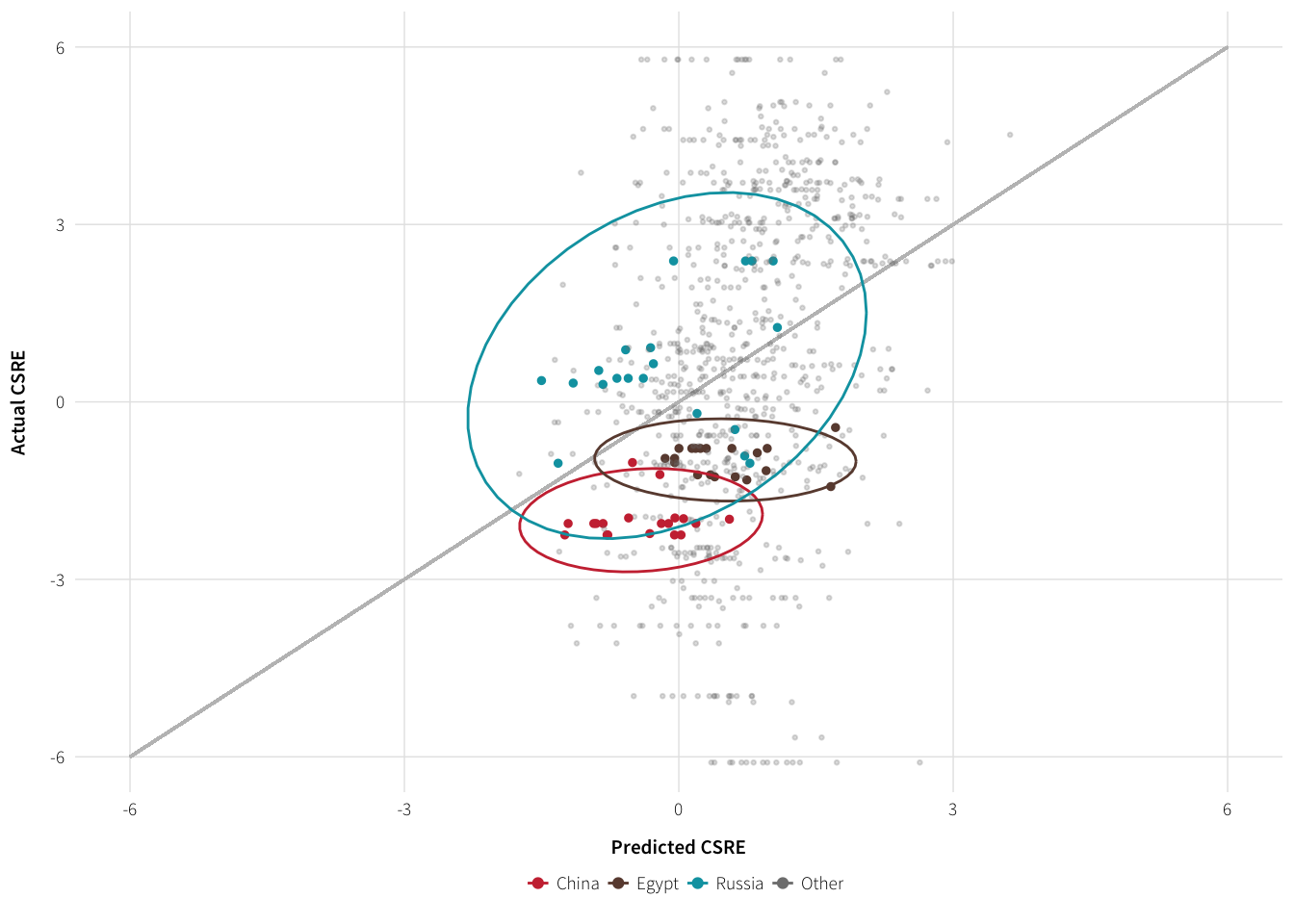
plotly::ggplotly(plot.lna.selection, tooltip="label")Bayesian tinkering?
See:
- https://cran.r-project.org/web/packages/rstanarm/vignettes/lm.html
- https://cran.r-project.org/web/packages/rstanarm/vignettes/continuous.html
Good, solid, interpretable results, but craaaaazy slow
# library(rstanarm)
# options(mc.cores = parallel::detectCores())  # Use all possible cores
#
# model.simple.b <- stan_glm(cs_env_sum.lead ~ icrg.stability + e_polity2,
#                           data=full.data, family=gaussian(),
#                           prior=cauchy(), prior_intercept=cauchy(),
#                           seed=my.seed)
# print(model.simple.b, digits=2)
# plot(model.simple.b, pars=c("icrg.stability", "e_polity2"))
# pp_check(model.simple.b, check="distributions", overlay=FALSE, nreps=5)