Survey analysis
Andrew Heiss
August 5, 2016
Load clean data
knitr::opts_chunk$set(cache=TRUE, fig.retina=2,
                      tidy.opts=list(width.cutoff=120),  # For code
                      options(width=120))  # For output

library(plyr)  # Because of productplots
library(dplyr)
library(tidyr)
library(purrr)
library(ggplot2)
library(ggstance)
library(productplots)
library(gridExtra)
library(stringr)
library(pander)
library(magrittr)
library(DT)
library(scales)
library(countrycode)
library(tm)

panderOptions('table.split.table', Inf)
panderOptions('table.split.cells', Inf)
panderOptions('keep.line.breaks', TRUE)
panderOptions('table.style', 'multiline')
panderOptions('table.alignment.default', 'left')

source(file.path(PROJHOME, "Analysis", "lib", "graphic_functions.R"))

# Load cleaned, country-based survey data (*with* the Q4\* loop)
survey.clean.all <- readRDS(file.path(PROJHOME, "Data", "data_processed",
                                      "survey_clean_all.rds"))

# Load cleaned, organization-based data (without the Q4 loop)
survey.orgs.clean <- readRDS(file.path(PROJHOME, "Data", "data_processed",
                                       "survey_orgs_clean.rds"))

# Load cleaned, country-based data (only the Q4 loop)
survey.countries.clean <- readRDS(file.path(PROJHOME, "Data", "data_processed",
                                            "survey_countries_clean.rds"))

# Load Robinson map projection
countries.ggmap <- readRDS(file.path(PROJHOME, "Data", "data_processed",
                                     "countries110_robinson_ggmap.rds"))

# All possible countries (to fix the South Sudan issue)
possible.countries <- data_frame(id = unique(as.character(countries.ggmap$id)))

# Survey responses
great.none.dk <- c("A great deal", "A lot", "A moderate amount",
                   "A little", "None at all", "Don't know", "Not applicable")
great.none <- great.none.dk[1:5]
# Useful functions#
# NB: xtabs() and productplots::prodplot(..., mosaic()) need to be mirror
# images of each other to get the same plot as vcd::mosaic()
#
# Example:
# prodplot(df, ~ x1 + x2 + x3, mosaic())
# xtabs(~ x3 + x2 + x1)
analyze.cat.var <- function(cat.table) {
cat.table.chi <- chisq.test(ftable(cat.table))
cat("Table counts\n")
ftable(cat.table) %>% print(method="col.compact")
cat("\nExpected values\n")
expected.values <- cat.table.chi$expected
# Add nice labels if possible
if(length(dim(cat.table)) == length(dim(expected.values))) {
dimnames(expected.values) <- dimnames(cat.table)
}
expected.values %>% print(method="col.compact")
cat("\nRow proporitions\n")
ftable(prop.table(cat.table, margin=1)) %>% print(method="col.compact")
cat("\nColumn proporitions\n")
ftable(prop.table(cat.table, margin=2)) %>% print(method="col.compact")
cat("\nChi-squared test for table\n")
cat.table.chi %>% print()
cat("Cramer's V\n")
vcd::assocstats(ftable(cat.table))$cramer %>% print()
cat("\nPearson residuals\n",
"2 is used as critical value by convention\n", sep="")
pearson.residuals <- cat.table.chi$residuals %>% print(method="col.compact")
cat("\nComponents of chi-squared\n",
"Critical value (0.05 with ",
cat.table.chi$parameter, " df) is ",
round(qchisq(0.95, cat.table.chi$parameter), 2), "\n", sep="")
components <- pearson.residuals^2 %>% print(method="col.compact")
cat("\np for components\n")
round(1-pchisq(components, cat.table.chi$parameter), 3) %>% print(method="col.compact")
}Organizational characteristics
How do respondents differ across the regime types of the countries they work in and the issues they work on?
Distribution of NGOs
Regime type
Regime types of the home countries for each organization
home.regime.type <- survey.orgs.clean %>%
  group_by(home.regime.type) %>%
  summarise(num = n()) %>%
  mutate(prop = num / sum(num))
home.regime.type
## # A tibble: 2 x 3
## home.regime.type num prop
## <fctr> <int> <dbl>
## 1 Democracy 569 0.8876755
## 2 Autocracy 72 0.1123245Regime types of the target countries for each country-organization
work.regime.type <- survey.countries.clean %>%
  group_by(target.regime.type) %>%
  summarise(num = n())%>%
  mutate(prop = num / sum(num))
work.regime.type
## # A tibble: 2 x 3
## target.regime.type num prop
## <fctr> <int> <dbl>
## 1 Democracy 440 0.6676783
## 2 Autocracy 219 0.3323217Most NGOs are based in democracies (only 11% are headquartered in autocracies), but a third of them answered questions about their work in autocracies.
Issues worked on across regime type
There are differences in potential contentiousness across regime type. In democracies, a quarter of INGOs work on more threatening issues, but in autocracies, nearly 40% do, which is a lot more than expected. Seen differently, across types of contentiousness, 70% of INGOs working on low contention issues work in democracies, in contrast to 58% of high contention INGOs.
This is most likely because autocracies are more in need of high contention issues like human rights advocacy, human trafficking, conflict prevention, and freedom of expression protection.
df.issue.regime <- survey.countries.clean %>%
  select(target.regime.type, potential.contentiousness)

plot.issue.regime <- prodplot(df.issue.regime,
                              ~ target.regime.type +
                                potential.contentiousness, mosaic("h")) +
  aes(fill=target.regime.type, linetype=potential.contentiousness) +
  scale_fill_manual(values=ath.palette("regime"), name=NULL) +
  scale_linetype_manual(values=c("blank", "dashed")) +
  guides(fill=FALSE, linetype=FALSE) +
  labs(title="Potential issue contentiousness across regime types",
       subtitle="Issue area of INGO + regime type of target country") +
  theme_ath() + theme(axis.title=element_blank(),
                      panel.grid=element_blank())
plot.issue.regime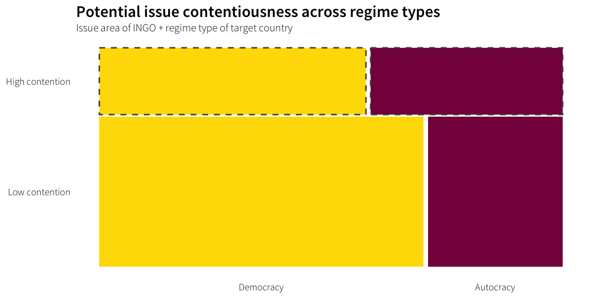
issue.regime.table <- survey.countries.clean %>%
  xtabs(~ target.regime.type + potential.contentiousness, .)

analyze.cat.var(issue.regime.table)
## Table counts
## potential.contentiousness Low contention High contention
## target.regime.type
## Democracy 322 118
## Autocracy 134 85
##
## Expected values
## potential.contentiousness
## target.regime.type Low contention High contention
## Democracy 304.4613 135.53869
## Autocracy 151.5387 67.46131
##
## Row proporitions
## potential.contentiousness Low contention High contention
## target.regime.type
## Democracy 0.7318182 0.2681818
## Autocracy 0.6118721 0.3881279
##
## Column proporitions
## potential.contentiousness Low contention High contention
## target.regime.type
## Democracy 0.7061404 0.5812808
## Autocracy 0.2938596 0.4187192
##
## Chi-squared test for table
##
## Pearson's Chi-squared test with Yates' continuity correction
##
## data: ftable(cat.table)
## X-squared = 9.3148, df = 1, p-value = 0.002273
##
## Cramer's V
## [1] 0.1223781
##
## Pearson residuals
## 2 is used as critical value by convention
## potential.contentiousness Low contention High contention
## target.regime.type
## Democracy 1.005151 -1.506488
## Autocracy -1.424740 2.135354
##
## Components of chi-squared
## Critical value (0.05 with 1 df) is 3.84
## potential.contentiousness Low contention High contention
## target.regime.type
## Democracy 1.010328 2.269506
## Autocracy 2.029883 4.559737
##
## p for components
## potential.contentiousness Low contention High contention
## target.regime.type
## Democracy 0.315 0.132
## Autocracy 0.154 0.033H1: Instrumental concerns
What is the relationship beween feelings of restriction and instrumental concerns? How do respondents working in different regime types and on different issues differ in the distribution of their instrumental characteristics? Do those differences help drive restrictions?
Things to check against relationship with government (Q4.11), types of regulation (Q4.16), overall level of restriction (Q4.17), changes in programming (Q4.19), type of changes (Q4.21), and attempts at changing regulations (Q4.23):
- Staffing (employees and volunteers)
- Collaboration (which kinds of institutions do they collaborate with + number of different types of collaborative relationships (i.e. collaboration only with governemnts vs. governments + IGOs + NGOs + businesses))
- Sources and mix of funding
- Time working in country
Employees
Relationship with government (Q4.11)
df.employees.relationship <- survey.clean.all %>%
  select(Q3.4.num, Q4.11, potential.contentiousness) %>%
  filter(!(Q4.11 %in% c("Don't know", "Prefer not to answer"))) %>%
  filter(!is.na(Q4.11)) %>%
  mutate(Q4.11 = droplevels(Q4.11),
         Q4.11 = factor(Q4.11, levels=rev(levels(Q4.11))))

df.employees.relationship.plot.means <- df.employees.relationship %>%
  group_by(Q4.11, potential.contentiousness) %>%
  summarise(average = mean(Q3.4.num, na.rm=TRUE),
            med = median(Q3.4.num, na.rm=TRUE),
num = n())ggplot(df.employees.relationship, aes(y=Q4.11, x=Q3.4.num)) +
geom_violinh(na.rm=TRUE) +
geom_point(alpha=0.2, size=0.5) +
geom_point(data=df.employees.relationship.plot.means,
aes(x=med, y=Q4.11)) +
scale_x_continuous(trans="log1p", breaks=c(0, 10^(0:5)), labels=comma) +
labs(x="Number of employees", y=NULL,
title="Relationship with government and # of employees") +
theme_ath() + facet_wrap(~ potential.contentiousness)## Warning: Removed 9 rows containing missing values (geom_point).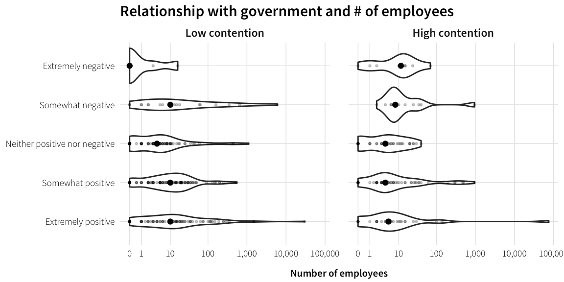
ggplot(df.employees.relationship.plot.means,
       aes(x=med, y=Q4.11, fill=potential.contentiousness)) +
  geom_barh(stat="identity", position="dodge") +
  scale_x_continuous(expand=c(0, 0)) +
  scale_fill_manual(values=ath.palette("contention"), name=NULL) +
  labs(x="Median number of employees", y=NULL,
       title="Median # of employees and relationship with government") +
  theme_ath()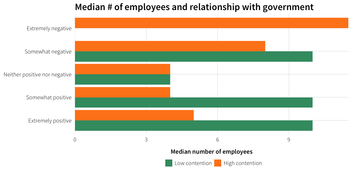
Types of regulation (Q4.16)
df.employees.reg.types <- survey.clean.all %>%
  select(Q3.4.num, starts_with("Q4.16"), -dplyr::contains("TEXT"),
         potential.contentiousness) %>%
  gather(regulation, response, starts_with("Q4.16")) %>%
  mutate(regulation = gsub("Q4\\.16_", "", regulation)) %>%
  filter(!(response %in% c("Don't know", "Not applicable"))) %>%
  filter(!is.na(response)) %>%
  mutate(response = factor(response, levels=great.none, ordered=TRUE))

df.employees.reg.types.plot.means <- df.employees.reg.types %>%
  group_by(regulation, response, potential.contentiousness) %>%
  summarise(average = mean(Q3.4.num, na.rm=TRUE),
            med = median(Q3.4.num, na.rm=TRUE),
num = n())ggplot(df.employees.reg.types, aes(y=response, x=Q3.4.num,
fill=potential.contentiousness)) +
geom_violinh(na.rm=TRUE) +
geom_point(alpha=0.2, size=0.5) +
geom_point(data=df.employees.reg.types.plot.means,
aes(x=med, y=response)) +
scale_x_continuous(trans="log1p", breaks=c(0, 10^(0:5)), labels=comma) +
scale_fill_manual(values=ath.palette("contention"), name=NULL) +
labs(x="Number of employees", y=NULL,
title="Types of regulation, perceptions of restriction, and # of employees (logged)") +
theme_ath() +
facet_wrap(~ regulation + potential.contentiousness, nrow=2)## Warning: Removed 46 rows containing missing values (geom_point).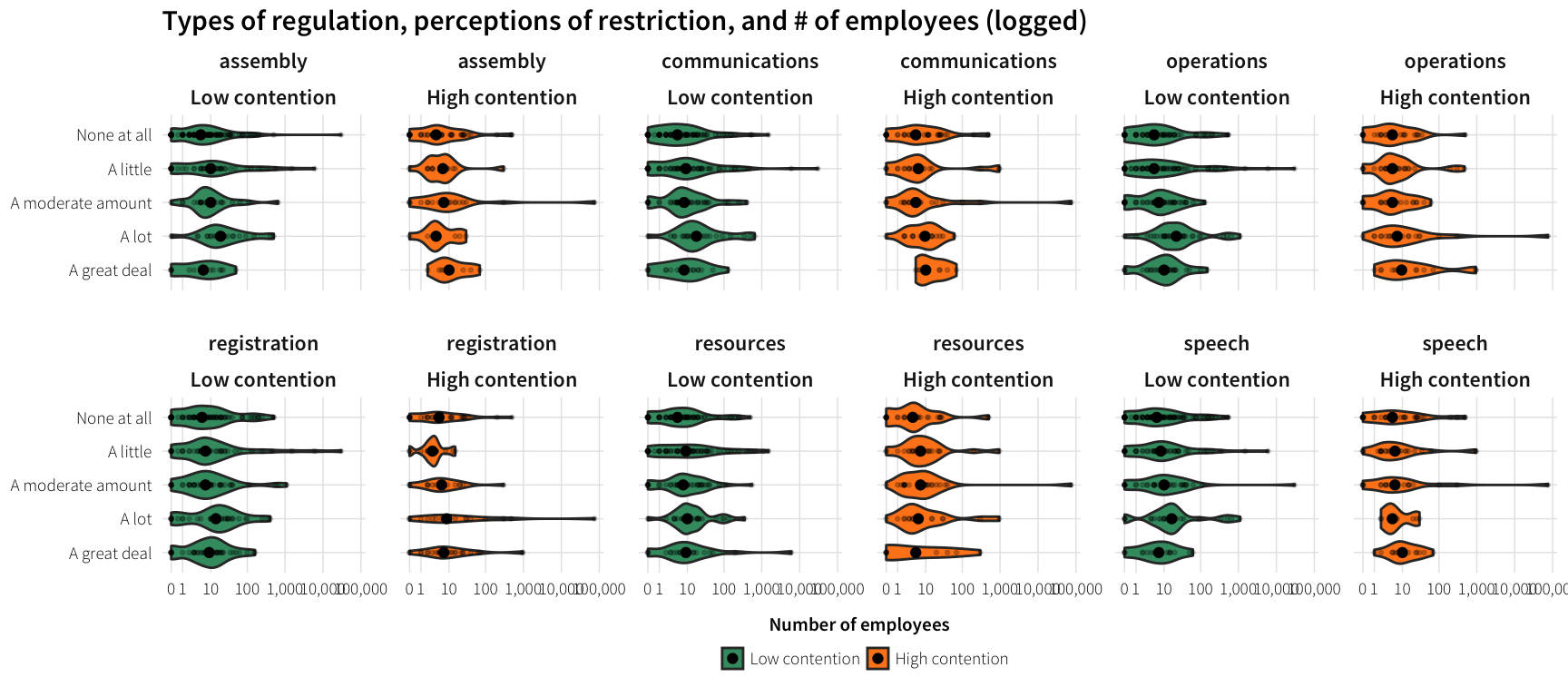
ggplot(df.employees.reg.types.plot.means,
       aes(x=med, y=response, fill=potential.contentiousness)) +
  geom_barh(stat="identity", position="dodge") +
  scale_x_continuous(expand=c(0, 0)) +
  scale_fill_manual(values=ath.palette("contention"), name=NULL) +
  labs(x="Median number of employees", y=NULL,
       title="Median # of employees and types of regulation") +
  theme_ath() + facet_wrap(~ regulation)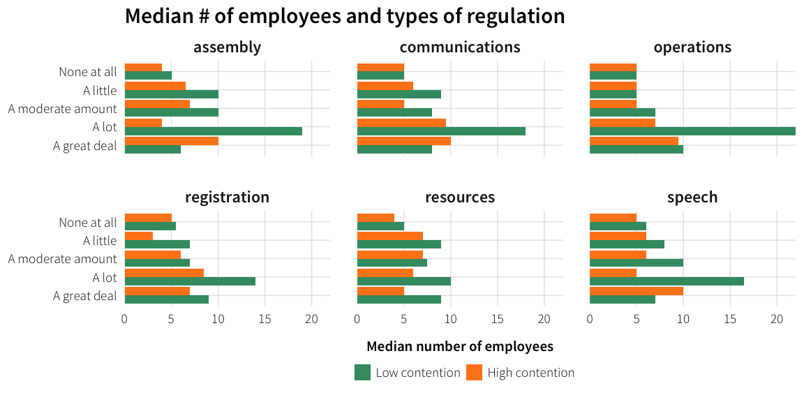
Overall perception of restriction (Q4.17)
df.employees.restriction <- survey.clean.all %>%
  select(Q3.4.num, Q4.17, potential.contentiousness) %>%
  filter(Q4.17 != "Don’t know") %>%
  mutate(Q4.17 = droplevels(Q4.17),
         Q4.17 = factor(Q4.17, levels=rev(levels(Q4.17))))

df.employees.restrictions.plot.means <- df.employees.restriction %>%
  group_by(Q4.17, potential.contentiousness) %>%
  summarise(average = mean(Q3.4.num, na.rm=TRUE),
            med = median(Q3.4.num, na.rm=TRUE),
num = n())ggplot(df.employees.restriction, aes(y=Q4.17, x=Q3.4.num)) +
geom_violinh(na.rm=TRUE) +
geom_point(alpha=0.2, size=0.5) +
geom_point(data=df.employees.restrictions.plot.means,
aes(x=med, y=Q4.17)) +
scale_x_continuous(trans="log1p", breaks=c(0, 10^(0:5)), labels=comma) +
labs(x="Number of employees", y=NULL,
title="Perceptions of restriction and # of employees") +
theme_ath() + facet_wrap(~ potential.contentiousness)## Warning: Removed 10 rows containing missing values (geom_point).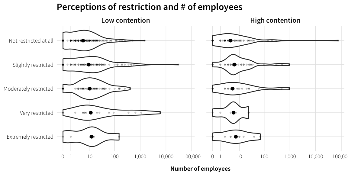
ggplot(df.employees.restrictions.plot.means,
       aes(x=med, y=Q4.17, fill=potential.contentiousness)) +
  geom_barh(stat="identity", position="dodge") +
  scale_x_continuous(expand=c(0, 0)) +
  scale_fill_manual(values=ath.palette("contention"), name=NULL) +
  labs(x="Median number of employees", y=NULL,
       title="Median # of employees and perceptions of restriction") +
  theme_ath()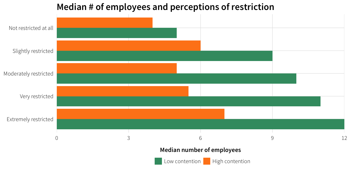
Changes in programming (Q4.19)
df.employees.changes <- survey.clean.all %>%
  select(Q3.4.num, Q4.19, potential.contentiousness) %>%
  filter(Q4.19 != "Don't know") %>%
  mutate(Q4.19 = droplevels(Q4.19),
         Q4.19 = factor(Q4.19, levels=rev(levels(Q4.19))))

df.employees.changes.plot.means <- df.employees.changes %>%
  group_by(Q4.19, potential.contentiousness) %>%
  summarise(average = mean(Q3.4.num, na.rm=TRUE),
            med = median(Q3.4.num, na.rm=TRUE),
num = n())ggplot(df.employees.changes, aes(y=Q4.19, x=Q3.4.num)) +
geom_violinh(na.rm=TRUE) +
geom_point(alpha=0.2, size=0.5) +
geom_point(data=df.employees.changes.plot.means,
aes(x=med, y=Q4.19)) +
scale_x_continuous(trans="log1p", breaks=c(0, 10^(0:5)), labels=comma) +
labs(x="Number of employees", y=NULL,
title="Changes in programming and # of employees") +
theme_ath() + facet_wrap(~ potential.contentiousness)## Warning: Removed 8 rows containing missing values (geom_point).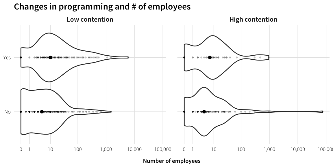
ggplot(df.employees.changes.plot.means,
       aes(x=med, y=Q4.19, fill=potential.contentiousness)) +
  geom_barh(stat="identity", position="dodge") +
  scale_x_continuous(expand=c(0, 0)) +
  scale_fill_manual(values=ath.palette("contention"), name=NULL) +
  labs(x="Median number of employees", y=NULL,
       title="Median # of employees and changes in programming") +
  theme_ath()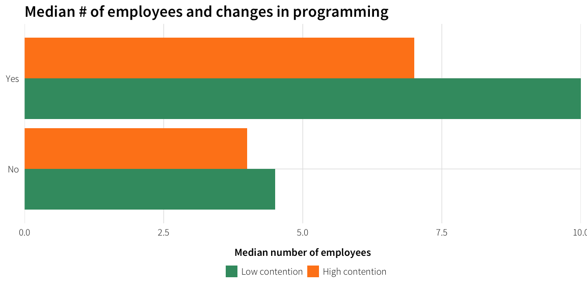
Attempts to change programming (Q4.23)
df.employees.change.attempt <- survey.clean.all %>%
  select(Q3.4.num, Q4.23, potential.contentiousness) %>%
  filter(Q4.23 != "Don't know") %>%
  mutate(Q4.23 = droplevels(Q4.23),
         Q4.23 = factor(Q4.23, levels=rev(levels(Q4.23))))

df.employees.change.attempt.plot.means <- df.employees.change.attempt %>%
  group_by(Q4.23, potential.contentiousness) %>%
  summarise(average = mean(Q3.4.num, na.rm=TRUE),
            med = median(Q3.4.num, na.rm=TRUE),
num = n())ggplot(df.employees.change.attempt, aes(y=Q4.23, x=Q3.4.num)) +
geom_violinh(na.rm=TRUE) +
geom_point(alpha=0.2, size=0.5) +
geom_point(data=df.employees.change.attempt.plot.means,
aes(x=med, y=Q4.23)) +
scale_x_continuous(trans="log1p", breaks=c(0, 10^(0:5)), labels=comma) +
labs(x="Number of employees", y=NULL,
title="Changes in programming and # of employees") +
theme_ath() + facet_wrap(~ potential.contentiousness)## Warning: Removed 8 rows containing missing values (geom_point).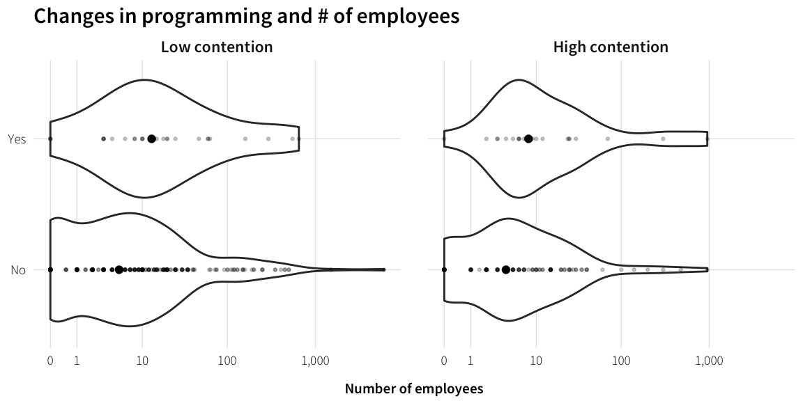
ggplot(df.employees.change.attempt.plot.means,
       aes(x=med, y=Q4.23, fill=potential.contentiousness)) +
  geom_barh(stat="identity", position="dodge") +
  scale_x_continuous(expand=c(0, 0)) +
  scale_fill_manual(values=ath.palette("contention"), name=NULL) +
  labs(x="Median number of employees", y=NULL,
       title="Median # of employees and changes in programming") +
  theme_ath()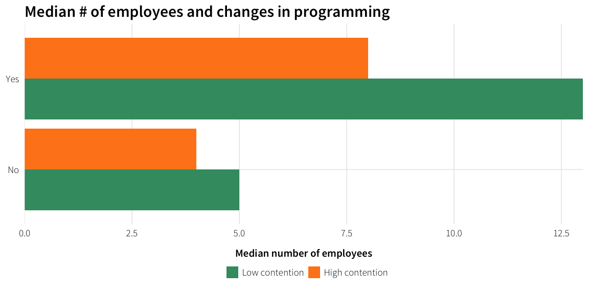
Volunteers
Overall perception of restriction (Q4.17)
df.volunteers.restriction <- survey.clean.all %>%
  select(Q3.5.num, Q4.17, potential.contentiousness) %>%
  filter(Q4.17 != "Don’t know") %>%
  mutate(Q4.17 = droplevels(Q4.17),
         Q4.17 = factor(Q4.17, levels=rev(levels(Q4.17))))

df.volunteers.restrictions.plot.means <- df.volunteers.restriction %>%
  group_by(Q4.17, potential.contentiousness) %>%
  summarise(average = mean(Q3.5.num, na.rm=TRUE),
            med = median(Q3.5.num, na.rm=TRUE),
num = n())ggplot(df.volunteers.restriction, aes(y=Q4.17, x=Q3.5.num)) +
geom_violinh(na.rm=TRUE) +
geom_point(alpha=0.2, size=0.5) +
geom_point(data=df.volunteers.restrictions.plot.means,
aes(x=med, y=Q4.17)) +
scale_x_continuous(trans="log1p", breaks=c(0, 10^(0:5)), labels=comma) +
labs(x="Number of volunteers", y=NULL,
title="Perceptions of restriction and # of volunteers") +
theme_ath() + facet_wrap(~ potential.contentiousness)## Warning: Removed 28 rows containing missing values (geom_point).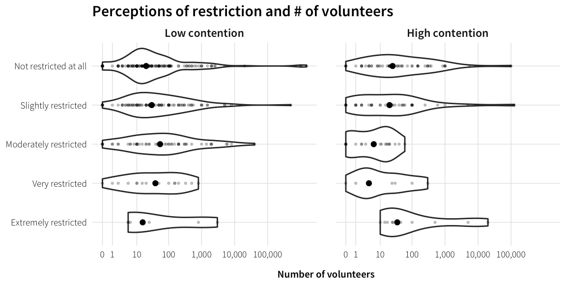
ggplot(df.volunteers.restrictions.plot.means,
       aes(x=med, y=Q4.17, fill=potential.contentiousness)) +
  geom_barh(stat="identity", position="dodge") +
  scale_x_continuous(expand=c(0, 0)) +
  scale_fill_manual(values=ath.palette("contention"), name=NULL) +
  labs(x="Median number of volunteers", y=NULL,
       title="Median # of volunteers and perceptions of restriction") +
  theme_ath()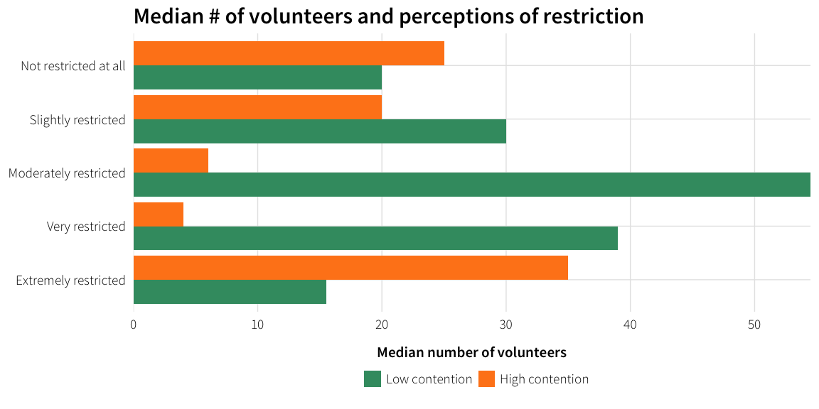
# TODO: Staffing, collaboration, funding, etc.

# TODO: Figure out how to deal with org-level regime type analysis, since organizations work in multiple countries and answered only for one. Proportion of countries they work in that are autocracies?
Relationships with governments
For regime-based questions, this analysis is more straightforward, since each country-organization response is limited to a single target country. The questions also deal with the organization’s specific actions in the country, not what they do in all countries.
Time spent working in the country
Regime type
Most NGOs working in democracies have been there for 10+ years, while most NGOs working in autocracies have only been there for 1-4 years, and the differences between time worked in country across regime types are significantly different from expected values. NGOs that work in autocracies tend to have less of a legacy or history of working there, are possibly less likely to have a history of working with the government.
df.time.country.regime <- survey.countries.clean %>%
  select(Q4.2, target.regime.type) %>%
  filter(Q4.2 != "Don't know") %>%
  mutate(Q4.2 = droplevels(Q4.2),
         Q4.2 = factor(Q4.2, levels=rev(levels(Q4.2))))

plot.time.country.regime <- prodplot(df.time.country.regime,
                                     ~ target.regime.type + Q4.2, mosaic("h"),
                                     colour=NA) +
  aes(fill=target.regime.type, colour="white") +
  scale_fill_manual(values=ath.palette("regime"), name=NULL) +
  guides(fill=FALSE) +
  labs(title="Length of time in country, by regime type",
       subtitle="Q4.2: How long has your organization worked in `target_country`?") +
  theme_ath() + theme(axis.title=element_blank(),
                      panel.grid=element_blank())
plot.time.country.regime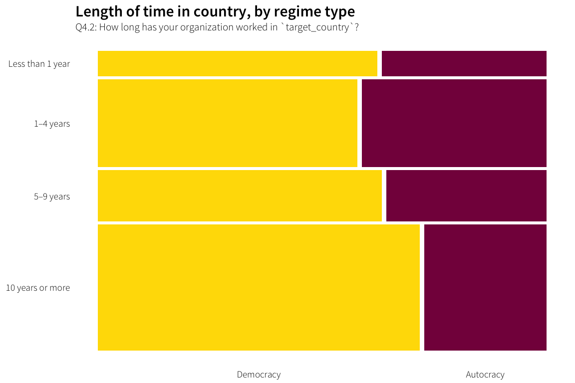
time.country.table <- survey.countries.clean %>%
  filter(Q4.2 != "Don't know") %>%
  mutate(Q4.2 = droplevels(Q4.2)) %>%
  xtabs(~ Q4.2 + target.regime.type, .)

analyze.cat.var(time.country.table)
## Table counts
## target.regime.type Democracy Autocracy
## Q4.2
## Less than 1 year 34 20
## 1–4 years 108 77
## 5–9 years 69 39
## 10 years or more 192 73
##
## Expected values
## target.regime.type
## Q4.2 Democracy Autocracy
## Less than 1 year 35.55882 18.44118
## 1–4 years 121.82190 63.17810
## 5–9 years 71.11765 36.88235
## 10 years or more 174.50163 90.49837
##
## Row proporitions
## target.regime.type Democracy Autocracy
## Q4.2
## Less than 1 year 0.6296296 0.3703704
## 1–4 years 0.5837838 0.4162162
## 5–9 years 0.6388889 0.3611111
## 10 years or more 0.7245283 0.2754717
##
## Column proporitions
## target.regime.type Democracy Autocracy
## Q4.2
## Less than 1 year 0.08436725 0.09569378
## 1–4 years 0.26799007 0.36842105
## 5–9 years 0.17121588 0.18660287
## 10 years or more 0.47642680 0.34928230
##
## Chi-squared test for table
##
## Pearson's Chi-squared test
##
## data: ftable(cat.table)
## X-squared = 10.115, df = 3, p-value = 0.01761
##
## Cramer's V
## [1] 0.1285602
##
## Pearson residuals
## 2 is used as critical value by convention
## target.regime.type Democracy Autocracy
## Q4.2
## Less than 1 year -0.2614106 0.3629967
## 1–4 years -1.2522900 1.7389388
## 5–9 years -0.2511105 0.3486938
## 10 years or more 1.3246396 -1.8394040
##
## Components of chi-squared
## Critical value (0.05 with 3 df) is 7.81
## target.regime.type Democracy Autocracy
## Q4.2
## Less than 1 year 0.06833552 0.13176658
## 1–4 years 1.56823035 3.02390827
## 5–9 years 0.06305649 0.12158739
## 10 years or more 1.75467018 3.38340709
##
## p for components
## target.regime.type Democracy Autocracy
## Q4.2
## Less than 1 year 0.995 0.988
## 1–4 years 0.667 0.388
## 5–9 years 0.996 0.989
## 10 years or more 0.625 0.336Potential contentiousness
NGOs working on low contention issues tend to have worked in their respecitve target countries for a long time. High contention issue NGOs are more than expected / more likely to work in their target countries for 4 years or less. This may be because there’s a burst of more contentious INGOs being allowed, or that more contentious INGOs get kicked out more regularly and can only stay in country for so long.
df.time.country.issue <- survey.countries.clean %>%
  select(Q4.2, potential.contentiousness) %>%
  filter(Q4.2 != "Don't know") %>%
  mutate(Q4.2 = droplevels(Q4.2),
         Q4.2 = factor(Q4.2, levels=rev(levels(Q4.2))))

plot.time.country.issue <- prodplot(df.time.country.issue,
                                     ~ potential.contentiousness + Q4.2, mosaic("h"),
                                     colour=NA) +
  aes(fill=potential.contentiousness, colour="white") +
  scale_fill_manual(values=ath.palette("contention"), name=NULL) +
  guides(fill=FALSE) +
  labs(title="Length of time in country, by potential contentiousness",
       subtitle="Q4.2: How long has your organization worked in `target_country`?") +
  theme_ath() + theme(axis.title=element_blank(),
                      panel.grid=element_blank())
plot.time.country.issue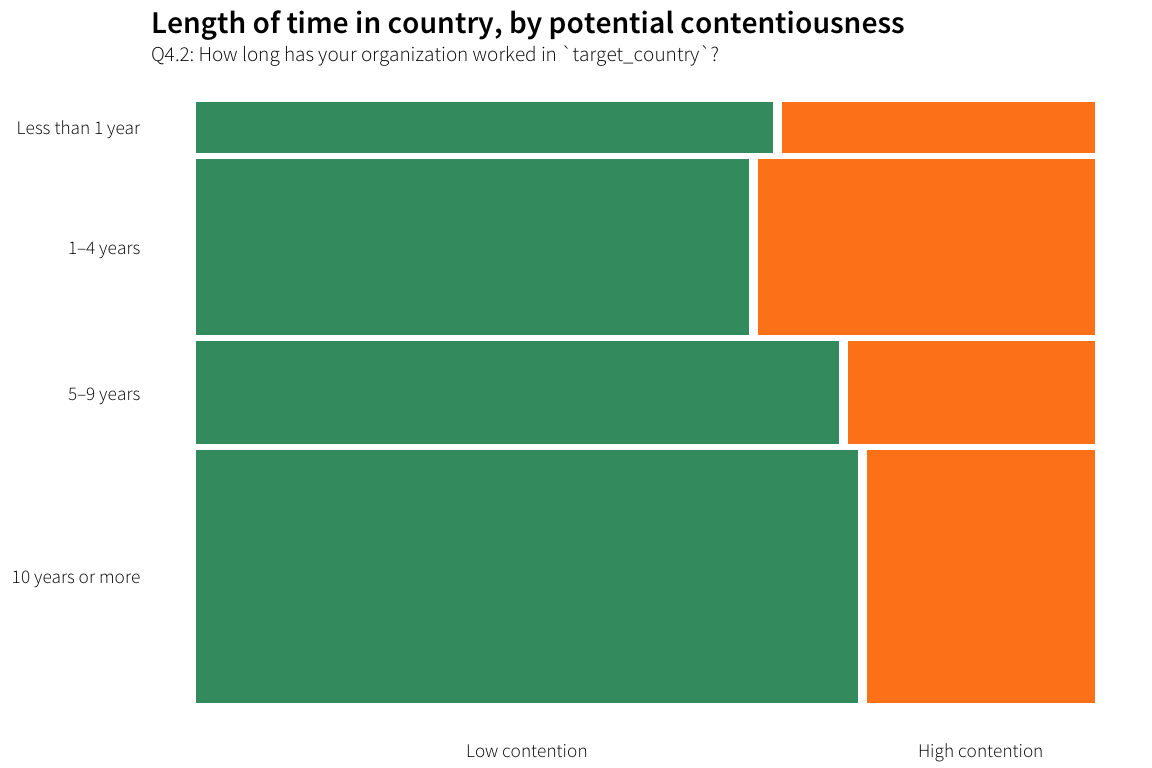
time.country.table.issue <- survey.countries.clean %>%
  filter(Q4.2 != "Don't know") %>%
  mutate(Q4.2 = droplevels(Q4.2)) %>%
  xtabs(~ Q4.2 + potential.contentiousness, .)

analyze.cat.var(time.country.table.issue)
## Table counts
## potential.contentiousness Low contention High contention
## Q4.2
## Less than 1 year 35 19
## 1–4 years 115 70
## 5–9 years 78 30
## 10 years or more 197 68
##
## Expected values
## potential.contentiousness
## Q4.2 Low contention High contention
## Less than 1 year 37.5000 16.50000
## 1–4 years 128.4722 56.52778
## 5–9 years 75.0000 33.00000
## 10 years or more 184.0278 80.97222
##
## Row proporitions
## potential.contentiousness Low contention High contention
## Q4.2
## Less than 1 year 0.6481481 0.3518519
## 1–4 years 0.6216216 0.3783784
## 5–9 years 0.7222222 0.2777778
## 10 years or more 0.7433962 0.2566038
##
## Column proporitions
## potential.contentiousness Low contention High contention
## Q4.2
## Less than 1 year 0.08235294 0.10160428
## 1–4 years 0.27058824 0.37433155
## 5–9 years 0.18352941 0.16042781
## 10 years or more 0.46352941 0.36363636
##
## Chi-squared test for table
##
## Pearson's Chi-squared test
##
## data: ftable(cat.table)
## X-squared = 8.5544, df = 3, p-value = 0.03584
##
## Cramer's V
## [1] 0.1182277
##
## Pearson residuals
## 2 is used as critical value by convention
## potential.contentiousness Low contention High contention
## Q4.2
## Less than 1 year -0.4082483 0.6154575
## 1–4 years -1.1885970 1.7918774
## 5–9 years 0.3464102 -0.5222330
## 10 years or more 0.9562527 -1.4416052
##
## Components of chi-squared
## Critical value (0.05 with 3 df) is 7.81
## potential.contentiousness Low contention High contention
## Q4.2
## Less than 1 year 0.1666667 0.3787879
## 1–4 years 1.4127628 3.2108245
## 5–9 years 0.1200000 0.2727273
## 10 years or more 0.9144193 2.0782257
##
## p for components
## potential.contentiousness Low contention High contention
## Q4.2
## Less than 1 year 0.983 0.945
## 1–4 years 0.703 0.360
## 5–9 years 0.989 0.965
## 10 years or more 0.822 0.556Regime type + contentiousness
When accounting for both regime type and main issue area, an interesting story emerges. Individually, I found that INGOs working in their target countries for 5+ years were most likely to work on non-contentious issues and work in democracies. Relatively few of the long-term INGOs work in either autocracies or on more contentious issues. This remains the case when accounting for both target-country regime type and main issue area. There are fewer low contention, long-term INGOs working in autocracies than expected and more low contention, long term INGOs working in democracies.
df.time.country.issue.regime <- survey.countries.clean %>%
  select(Q4.2, potential.contentiousness, target.regime.type) %>%
  filter(Q4.2 != "Don't know") %>%
  mutate(Q4.2 = droplevels(Q4.2),
         Q4.2 = factor(Q4.2, levels=rev(levels(Q4.2))))

plot.time.country.issue.regime <- prodplot(df.time.country.issue.regime,
                                    ~ target.regime.type + potential.contentiousness +
                                      Q4.2, mosaic("v")) +
  aes(fill=target.regime.type, linetype=potential.contentiousness) +
  scale_fill_manual(values=ath.palette("regime")) +
  scale_linetype_manual(values=c("blank", "dashed")) +
  guides(fill=FALSE, linetype=FALSE) +
  labs(title="Length of time in country",
       subtitle="Issue area of INGO + regime type of target country") +
  theme_ath() + theme(axis.title=element_blank(),
                      panel.grid=element_blank())
plot.time.country.issue.regime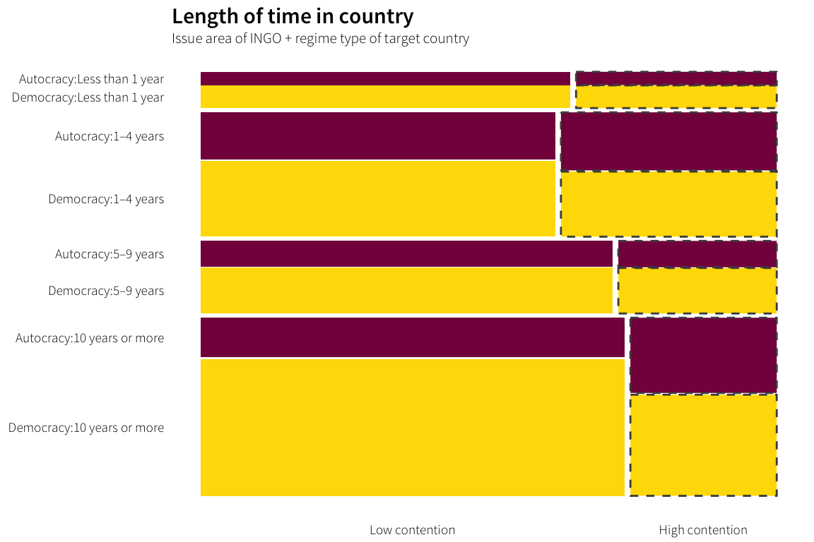
time.country.table.issue.regime <- survey.countries.clean %>%
  filter(Q4.2 != "Don't know") %>%
  mutate(Q4.2 = droplevels(Q4.2)) %>%
  xtabs(~ Q4.2 + potential.contentiousness + target.regime.type, .)

analyze.cat.var(time.country.table.issue.regime)
## Table counts
## target.regime.type Democracy Autocracy
## Q4.2 potential.contentiousness
## Less than 1 year Low contention 22 13
## High contention 12 7
## 1–4 years Low contention 71 44
## High contention 37 33
## 5–9 years Low contention 50 28
## High contention 19 11
## 10 years or more Low contention 153 44
## High contention 39 29
##
## Expected values
## [,1] [,2]
## [1,] 23.04739 11.952614
## [2,] 12.51144 6.488562
## [3,] 75.72712 39.272876
## [4,] 46.09477 23.905229
## [5,] 51.36275 26.637255
## [6,] 19.75490 10.245098
## [7,] 129.72386 67.276144
## [8,] 44.77778 23.222222
##
## Row proporitions
## target.regime.type Democracy Autocracy
## Q4.2 potential.contentiousness
## Less than 1 year Low contention 0.4074074 0.2407407
## High contention 0.2222222 0.1296296
## 1–4 years Low contention 0.3837838 0.2378378
## High contention 0.2000000 0.1783784
## 5–9 years Low contention 0.4629630 0.2592593
## High contention 0.1759259 0.1018519
## 10 years or more Low contention 0.5773585 0.1660377
## High contention 0.1471698 0.1094340
##
## Column proporitions
## target.regime.type Democracy Autocracy
## Q4.2 potential.contentiousness
## Less than 1 year Low contention 0.05176471 0.03058824
## High contention 0.06417112 0.03743316
## 1–4 years Low contention 0.16705882 0.10352941
## High contention 0.19786096 0.17647059
## 5–9 years Low contention 0.11764706 0.06588235
## High contention 0.10160428 0.05882353
## 10 years or more Low contention 0.36000000 0.10352941
## High contention 0.20855615 0.15508021
##
## Chi-squared test for table
##
## Pearson's Chi-squared test
##
## data: ftable(cat.table)
## X-squared = 20.922, df = 7, p-value = 0.003887
##
## Cramer's V
## [1] 0.1848957
##
## Pearson residuals
## 2 is used as critical value by convention
## target.regime.type Democracy Autocracy
## Q4.2 potential.contentiousness
## Less than 1 year Low contention -0.2181704 0.3029529
## High contention -0.1445903 0.2007792
## 1–4 years Low contention -0.5432144 0.7543114
## High contention -1.3395717 1.8601387
## 5–9 years Low contention -0.1901475 0.2640401
## High contention -0.1698451 0.2358482
## 10 years or more Low contention 2.0436245 -2.8377915
## High contention -0.8634348 1.1989717
##
## Components of chi-squared
## Critical value (0.05 with 7 df) is 14.07
## target.regime.type Democracy Autocracy
## Q4.2 potential.contentiousness
## Less than 1 year Low contention 0.04759831 0.09178048
## High contention 0.02090637 0.04031228
## 1–4 years Low contention 0.29508189 0.56898566
## High contention 1.79445221 3.46011598
## 5–9 years Low contention 0.03615605 0.06971718
## High contention 0.02884737 0.05562436
## 10 years or more Low contention 4.17640121 8.05306070
## High contention 0.74551971 1.43753323
##
## p for components
## target.regime.type Democracy Autocracy
## Q4.2 potential.contentiousness
## Less than 1 year Low contention 1.000 1.000
## High contention 1.000 1.000
## 1–4 years Low contention 1.000 0.999
## High contention 0.970 0.839
## 5–9 years Low contention 1.000 1.000
## High contention 1.000 1.000
## 10 years or more Low contention 0.759 0.328
## High contention 0.998 0.984How NGOs operate in country
Regime type
NGOs in autocracies definitely pursue different operational strategies. The most common strategy for these NGOs is to provide funding to domestic NGOs, while the least common is to maintain an office staffed by foreigners (difference is statistically significant). International NGOs seem to be more likely to take a hands off approach to advocacy in target countries that are autocracies.
what.do <- c("Maintain a physical office staffed primarily by foreigners",
             "Maintain a physical office staffed primarily by people from target_country",
             "Provide funding to domestic NGOs", "Partner with domestic NGOs")
what.do.short <- c("Maintain a physical office staffed\nprimarily by foreigners",
                   "Maintain a physical office staffed\nprimarily by people from target_country",
                   "Provide funding to domestic NGOs", "Partner with domestic NGOs")

df.operations.regime <- survey.countries.clean %>%
  unnest(Q4.3_value) %>%
  select(Q4.3_value, target.regime.type) %>%
  filter(!is.na(Q4.3_value), Q4.3_value != "Don't know") %>%
  mutate(Q4.3 = factor(Q4.3_value, levels=what.do,
                       labels=what.do.short, ordered=TRUE))

plot.operations.regime <- prodplot(df.operations.regime,
                                     ~ target.regime.type + Q4.3, mosaic("h"),
                                     colour=NA) +
  aes(fill=target.regime.type, colour="white") +
  scale_fill_manual(values=ath.palette("regime"), name=NULL) +
  guides(fill=FALSE) +
  labs(title="How INGOs work in the target country, by regime type",
       subtitle="Q4.3: What does your organization do in `target_country`?\n(multiple answers allowed)") +
  theme_ath() + theme(axis.title=element_blank(),
                      panel.grid=element_blank())
plot.operations.regime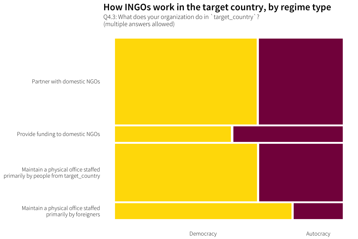
operations.table <- survey.countries.clean %>%
  unnest(Q4.3_value) %>%
  filter(Q4.3_value != "Don't know") %>%
  xtabs(~ Q4.3_value + target.regime.type, .)

analyze.cat.var(operations.table)
## Table counts
## target.regime.type Democracy Autocracy
## Q4.3_value
## Maintain a physical office staffed primarily by foreigners 54 15
## Maintain a physical office staffed primarily by people from target_country 158 93
## Partner with domestic NGOs 235 139
## Provide funding to domestic NGOs 35 33
##
## Expected values
## target.regime.type
## Q4.3_value Democracy Autocracy
## Maintain a physical office staffed primarily by foreigners 43.64567 25.35433
## Maintain a physical office staffed primarily by people from target_country 158.76903 92.23097
## Partner with domestic NGOs 236.57218 137.42782
## Provide funding to domestic NGOs 43.01312 24.98688
##
## Row proporitions
## target.regime.type Democracy Autocracy
## Q4.3_value
## Maintain a physical office staffed primarily by foreigners 0.7826087 0.2173913
## Maintain a physical office staffed primarily by people from target_country 0.6294821 0.3705179
## Partner with domestic NGOs 0.6283422 0.3716578
## Provide funding to domestic NGOs 0.5147059 0.4852941
##
## Column proporitions
## target.regime.type Democracy Autocracy
## Q4.3_value
## Maintain a physical office staffed primarily by foreigners 0.11203320 0.05357143
## Maintain a physical office staffed primarily by people from target_country 0.32780083 0.33214286
## Partner with domestic NGOs 0.48755187 0.49642857
## Provide funding to domestic NGOs 0.07261411 0.11785714
##
## Chi-squared test for table
##
## Pearson's Chi-squared test
##
## data: ftable(cat.table)
## X-squared = 10.786, df = 3, p-value = 0.01294
##
## Cramer's V
## [1] 0.1189748
##
## Pearson residuals
## 2 is used as critical value by convention
## target.regime.type Democracy Autocracy
## Q4.3_value
## Maintain a physical office staffed primarily by foreigners 1.56729754 -2.05634489
## Maintain a physical office staffed primarily by people from target_country -0.06103230 0.08007635
## Partner with domestic NGOs -0.10221627 0.13411104
## Provide funding to domestic NGOs -1.22180343 1.60304547
##
## Components of chi-squared
## Critical value (0.05 with 3 df) is 7.81
## target.regime.type Democracy Autocracy
## Q4.3_value
## Maintain a physical office staffed primarily by foreigners 2.456421592 4.228554311
## Maintain a physical office staffed primarily by people from target_country 0.003724942 0.006412221
## Partner with domestic NGOs 0.010448165 0.017985770
## Provide funding to domestic NGOs 1.492803613 2.569754792
##
## p for components
## target.regime.type Democracy Autocracy
## Q4.3_value
## Maintain a physical office staffed primarily by foreigners 0.483 0.238
## Maintain a physical office staffed primarily by people from target_country 1.000 1.000
## Partner with domestic NGOs 1.000 0.999
## Provide funding to domestic NGOs 0.684 0.463Potential contentiousness
There’s an overall significant difference in frequencies, driven primarily by more high contention INGOs working with foreigners. The individual cell effects, however, aren’t particularly significant. In general, more INGOs than expected use foreigners in their target countries).
df.operations.issue <- survey.countries.clean %>%
  unnest(Q4.3_value) %>%
  select(Q4.3_value, potential.contentiousness) %>%
  filter(!is.na(Q4.3_value), Q4.3_value != "Don't know") %>%
  mutate(Q4.3 = factor(Q4.3_value, levels=what.do,
                       labels=what.do.short, ordered=TRUE))

plot.operations.issue <- prodplot(df.operations.issue,
                                  ~ potential.contentiousness + Q4.3, mosaic("h"),
                                  colour=NA) +
  aes(fill=potential.contentiousness, colour="white") +
  scale_fill_manual(values=ath.palette("contention"), name=NULL) +
  guides(fill=FALSE) +
  labs(title="How INGOs work in the target country, by issue",
       subtitle="Q4.3: What does your organization do in `target_country`?\n(multiple answers allowed)") +
  theme_ath() + theme(axis.title=element_blank(),
                      panel.grid=element_blank())
plot.operations.issue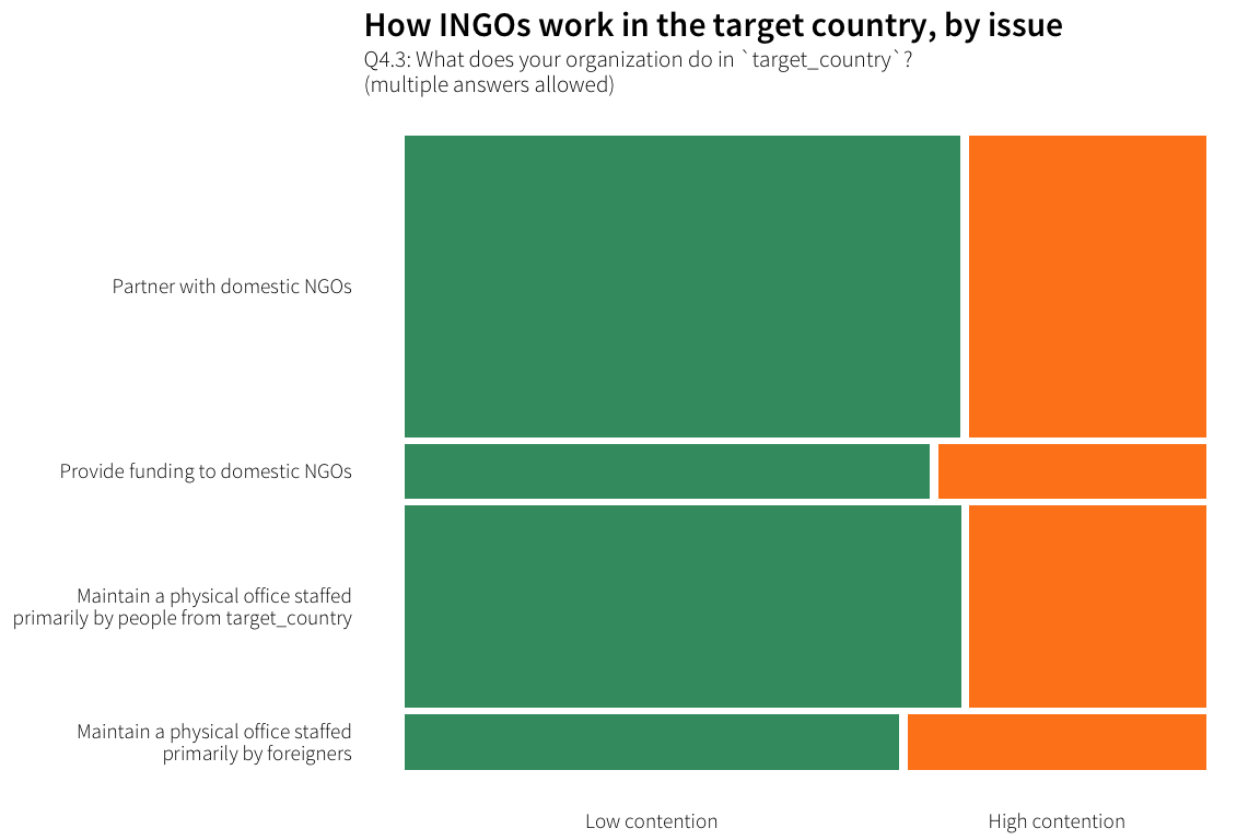
operations.table.issue <- survey.countries.clean %>%
  unnest(Q4.3_value) %>%
  filter(Q4.3_value != "Don't know") %>%
  xtabs(~ Q4.3_value + potential.contentiousness, .)

analyze.cat.var(operations.table.issue)
## Table counts
## potential.contentiousness Low contention High contention
## Q4.3_value
## Maintain a physical office staffed primarily by foreigners 43 26
## Maintain a physical office staffed primarily by people from target_country 176 75
## Partner with domestic NGOs 262 112
## Provide funding to domestic NGOs 45 23
##
## Expected values
## potential.contentiousness
## Q4.3_value Low contention High contention
## Maintain a physical office staffed primarily by foreigners 47.62992 21.37008
## Maintain a physical office staffed primarily by people from target_country 173.26247 77.73753
## Partner with domestic NGOs 258.16798 115.83202
## Provide funding to domestic NGOs 46.93963 21.06037
##
## Row proporitions
## potential.contentiousness Low contention High contention
## Q4.3_value
## Maintain a physical office staffed primarily by foreigners 0.6231884 0.3768116
## Maintain a physical office staffed primarily by people from target_country 0.7011952 0.2988048
## Partner with domestic NGOs 0.7005348 0.2994652
## Provide funding to domestic NGOs 0.6617647 0.3382353
##
## Column proporitions
## potential.contentiousness Low contention High contention
## Q4.3_value
## Maintain a physical office staffed primarily by foreigners 0.08174905 0.11016949
## Maintain a physical office staffed primarily by people from target_country 0.33460076 0.31779661
## Partner with domestic NGOs 0.49809886 0.47457627
## Provide funding to domestic NGOs 0.08555133 0.09745763
##
## Chi-squared test for table
##
## Pearson's Chi-squared test
##
## data: ftable(cat.table)
## X-squared = 2.0352, df = 3, p-value = 0.5651
##
## Cramer's V
## [1] 0.05168098
##
## Pearson residuals
## 2 is used as critical value by convention
## potential.contentiousness Low contention High contention
## Q4.3_value
## Maintain a physical office staffed primarily by foreigners -0.6708627 1.0015452
## Maintain a physical office staffed primarily by people from target_country 0.2079731 -0.3104874
## Partner with domestic NGOs 0.2384936 -0.3560521
## Provide funding to domestic NGOs -0.2831064 0.4226555
##
## Components of chi-squared
## Critical value (0.05 with 3 df) is 7.81
## potential.contentiousness Low contention High contention
## Q4.3_value
## Maintain a physical office staffed primarily by foreigners 0.45005682 1.00309274
## Maintain a physical office staffed primarily by people from target_country 0.04325279 0.09640241
## Partner with domestic NGOs 0.05687919 0.12677310
## Provide funding to domestic NGOs 0.08014921 0.17863764
##
## p for components
## potential.contentiousness Low contention High contention
## Q4.3_value
## Maintain a physical office staffed primarily by foreigners 0.930 0.801
## Maintain a physical office staffed primarily by people from target_country 0.998 0.992
## Partner with domestic NGOs 0.996 0.988
## Provide funding to domestic NGOs 0.994 0.981Registration
Regime type
There’s a slight difference in how NGOs register across regimes, with more NGOs registering in autocracies than in democracies, perhaps because they are more likely to be required to register in autocracies. The difference is not significant, though.
df.registered.regime <- survey.countries.clean %>%
  select(Q4.4, target.regime.type) %>%
  filter(Q4.4 != "Don't know") %>%
  mutate(Q4.4 = droplevels(Q4.4),
         Q4.4 = factor(Q4.4, levels=rev(levels(Q4.4))))

plot.registered.regime <- prodplot(df.registered.regime,
                                   ~ target.regime.type + Q4.4, mosaic("h"),
                                   colour=NA) +
  aes(fill=target.regime.type, colour="white") +
  scale_fill_manual(values=ath.palette("regime"), name=NULL) +
  guides(fill=FALSE) +
  labs(title="Registration status, by regime type",
       subtitle="Q4.4: Is your organization registered with the national government in `target_country`?") +
  theme_ath() + theme(axis.title=element_blank(),
                      panel.grid=element_blank())
plot.registered.regime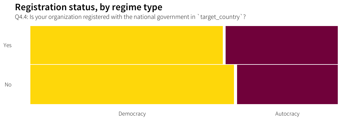
registered.table <- survey.countries.clean %>%
  filter(Q4.4 != "Don't know") %>%
  mutate(Q4.4 = droplevels(Q4.4)) %>%
  xtabs(~ Q4.4 + target.regime.type, .)

analyze.cat.var(registered.table)
## Table counts
## target.regime.type Democracy Autocracy
## Q4.4
## Yes 180 105
## No 198 98
##
## Expected values
## target.regime.type
## Q4.4 Democracy Autocracy
## Yes 185.4217 99.57831
## No 192.5783 103.42169
##
## Row proporitions
## target.regime.type Democracy Autocracy
## Q4.4
## Yes 0.6315789 0.3684211
## No 0.6689189 0.3310811
##
## Column proporitions
## target.regime.type Democracy Autocracy
## Q4.4
## Yes 0.4761905 0.5172414
## No 0.5238095 0.4827586
##
## Chi-squared test for table
##
## Pearson's Chi-squared test with Yates' continuity correction
##
## data: ftable(cat.table)
## X-squared = 0.73389, df = 1, p-value = 0.3916
##
## Cramer's V
## [1] 0.03915149
##
## Pearson residuals
## 2 is used as critical value by convention
## target.regime.type Democracy Autocracy
## Q4.4
## Yes -0.3981568 0.5433154
## No 0.3906886 -0.5331245
##
## Components of chi-squared
## Critical value (0.05 with 1 df) is 3.84
## target.regime.type Democracy Autocracy
## Q4.4
## Yes 0.1585289 0.2951917
## No 0.1526376 0.2842217
##
## p for components
## target.regime.type Democracy Autocracy
## Q4.4
## Yes 0.691 0.587
## No 0.696 0.594Potential contentiousness
There is no significant difference in the registration status of low and high contentious INGOs.
df.registered.issue <- survey.countries.clean %>%
  select(Q4.4, potential.contentiousness) %>%
  filter(Q4.4 != "Don't know") %>%
  mutate(Q4.4 = droplevels(Q4.4),
         Q4.4 = factor(Q4.4, levels=rev(levels(Q4.4))))

plot.registered.issue <- prodplot(df.registered.issue,
                                  ~ potential.contentiousness + Q4.4, mosaic("h"),
                                  colour=NA) +
  aes(fill=potential.contentiousness, colour="white") +
  scale_fill_manual(values=ath.palette("contention"), name=NULL) +
  guides(fill=FALSE) +
  labs(title="Registration status, by issue",
       subtitle="Q4.4: Is your organization registered with the national government in `target_country`?") +
  theme_ath() + theme(axis.title=element_blank(),
                      panel.grid=element_blank())
plot.registered.issue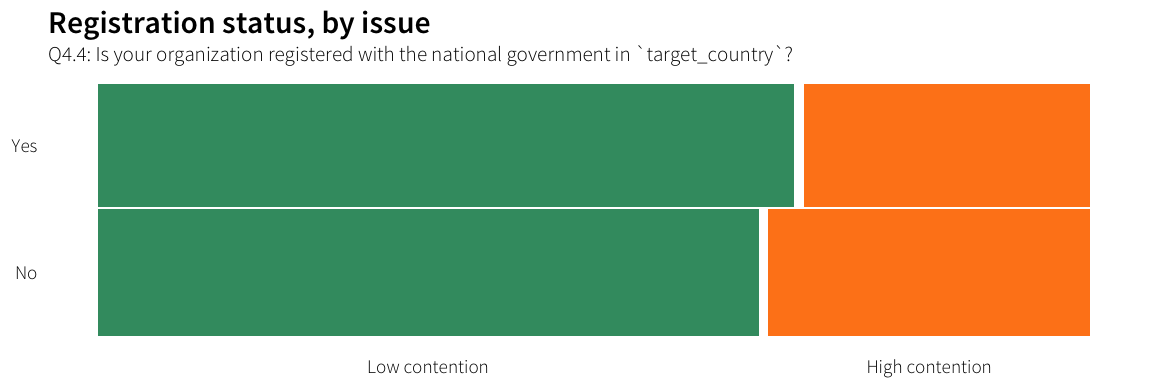
registered.table.issue <- survey.countries.clean %>%
  filter(Q4.4 != "Don't know") %>%
  mutate(Q4.4 = droplevels(Q4.4)) %>%
  xtabs(~ Q4.4 + potential.contentiousness, .)

analyze.cat.var(registered.table.issue)
## Table counts
## potential.contentiousness Low contention High contention
## Q4.4
## Yes 202 83
## No 199 97
##
## Expected values
## potential.contentiousness
## Q4.4 Low contention High contention
## Yes 196.704 88.29604
## No 204.296 91.70396
##
## Row proporitions
## potential.contentiousness Low contention High contention
## Q4.4
## Yes 0.7087719 0.2912281
## No 0.6722973 0.3277027
##
## Column proporitions
## potential.contentiousness Low contention High contention
## Q4.4
## Yes 0.5037406 0.4611111
## No 0.4962594 0.5388889
##
## Chi-squared test for table
##
## Pearson's Chi-squared test with Yates' continuity correction
##
## data: ftable(cat.table)
## X-squared = 0.74087, df = 1, p-value = 0.3894
##
## Cramer's V
## [1] 0.03943218
##
## Pearson residuals
## 2 is used as critical value by convention
## potential.contentiousness Low contention High contention
## Q4.4
## Yes 0.3776112 -0.5636127
## No -0.3705283 0.5530410
##
## Components of chi-squared
## Critical value (0.05 with 1 df) is 3.84
## potential.contentiousness Low contention High contention
## Q4.4
## Yes 0.1425902 0.3176592
## No 0.1372912 0.3058543
##
## p for components
## potential.contentiousness Low contention High contention
## Q4.4
## Yes 0.706 0.573
## No 0.711 0.580Contact with government
Frequency of contact with government
There’s a dramatic difference in how NGOs report to the government in autocracies. INGOs that work in autocracies report the most often and are the least likely to never report, possibly reflective of stricter reporting requirements.
freq.collapsed <- c("More than once a year", "Once a year",
                    "Regularly but not often", "Never")

df.freq.report.regime <- survey.countries.clean %>%
  filter(!is.na(Q4.8.clean)) %>%
  mutate(Q4.8.collapsed = case_when(
    .$Q4.8.clean == "Once a week" ~ freq.collapsed[1],
    .$Q4.8.clean == "More than once a month,\nless than once a week" ~ freq.collapsed[1],
    .$Q4.8.clean == "Once a month" ~ freq.collapsed[1],
    .$Q4.8.clean == "More than once a year,\nless than once a month" ~ freq.collapsed[1],
    .$Q4.8.clean == "Once a year" ~ freq.collapsed[2],
    .$Q4.8.clean == "As necessary/depends" ~ freq.collapsed[3],
    .$Q4.8.clean == "Once every 2+ years" ~ freq.collapsed[3],
    .$Q4.8.clean == "Never" ~ freq.collapsed[4],
    TRUE ~ NA_character_)
    ) %>%
  filter(!is.na(Q4.8.collapsed)) %>%
  mutate(Q4.8.collapsed = factor(Q4.8.collapsed, levels=rev(freq.collapsed),
                                 ordered=TRUE))

plot.freq.report.regime <- prodplot(df.freq.report.regime,
                                   ~ target.regime.type + Q4.8.collapsed, mosaic("h"),
                                   colour=NA) +
  aes(fill=target.regime.type, colour="white") +
  scale_fill_manual(values=ath.palette("regime"), name=NULL) +
  guides(fill=FALSE) +
  labs(title="Frequency of reporting to government, by regime type",
       subtitle="Q4.8: How often is your organization required to report to the government of  `target_country`?") +
  theme_ath() + theme(axis.title=element_blank(),
                      panel.grid=element_blank())
plot.freq.report.regime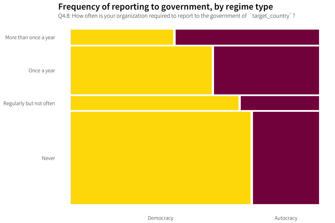
freq.report.table <- df.freq.report.regime %>%
  xtabs(~ Q4.8.collapsed + target.regime.type, .)

analyze.cat.var(freq.report.table)
## Table counts
## target.regime.type Democracy Autocracy
## Q4.8.collapsed
## Never 212 78
## Regularly but not often 30 14
## Once a year 86 64
## More than once a year 20 28
##
## Expected values
## target.regime.type
## Q4.8.collapsed Democracy Autocracy
## Never 189.69925 100.30075
## Regularly but not often 28.78195 15.21805
## Once a year 98.12030 51.87970
## More than once a year 31.39850 16.60150
##
## Row proporitions
## target.regime.type Democracy Autocracy
## Q4.8.collapsed
## Never 0.7310345 0.2689655
## Regularly but not often 0.6818182 0.3181818
## Once a year 0.5733333 0.4266667
## More than once a year 0.4166667 0.5833333
##
## Column proporitions
## target.regime.type Democracy Autocracy
## Q4.8.collapsed
## Never 0.60919540 0.42391304
## Regularly but not often 0.08620690 0.07608696
## Once a year 0.24712644 0.34782609
## More than once a year 0.05747126 0.15217391
##
## Chi-squared test for table
##
## Pearson's Chi-squared test
##
## data: ftable(cat.table)
## X-squared = 24.022, df = 3, p-value = 2.472e-05
##
## Cramer's V
## [1] 0.2124944
##
## Pearson residuals
## 2 is used as critical value by convention
## target.regime.type Democracy Autocracy
## Q4.8.collapsed
## Never 1.6191486 -2.2267292
## Regularly but not often 0.2270404 -0.3122367
## Once a year -1.2235845 1.6827309
## More than once a year -2.0341976 2.7975242
##
## Components of chi-squared
## Critical value (0.05 with 3 df) is 7.81
## target.regime.type Democracy Autocracy
## Q4.8.collapsed
## Never 2.62164210 4.95832309
## Regularly but not often 0.05154736 0.09749175
## Once a year 1.49715899 2.83158331
## More than once a year 4.13795984 7.82614144
##
## p for components
## target.regime.type Democracy Autocracy
## Q4.8.collapsed
## Never 0.454 0.175
## Regularly but not often 0.997 0.992
## Once a year 0.683 0.418
## More than once a year 0.247 0.050Government involvement
Members of the government aren’t typically directly invovled in INGO work, but when they are, it is more likely to occur with INGOs working in autocracies.
df.involvement.regime <- survey.countries.clean %>%
  select(Q4.9, target.regime.type) %>%
  filter(Q4.9 != "Don't know") %>%
  mutate(Q4.9 = droplevels(Q4.9),
         Q4.9 = factor(Q4.9, levels=rev(levels(Q4.9))))

plot.involvement.regime <- prodplot(df.involvement.regime,
                                   ~ target.regime.type + Q4.9, mosaic("h"),
                                   colour=NA) +
  aes(fill=target.regime.type, colour="white") +
  scale_fill_manual(values=ath.palette("regime"), name=NULL) +
  guides(fill=FALSE) +
  labs(title="Government involvement, by regime type",
       subtitle="Q4.9: Are members of the government or ruling party of `target_country` involved in your work?") +
  theme_ath() + theme(axis.title=element_blank(),
                      panel.grid=element_blank())
plot.involvement.regime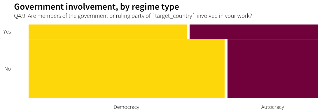
involvement.table <- survey.countries.clean %>%
  filter(Q4.9 != "Don't know") %>%
  mutate(Q4.9 = droplevels(Q4.9)) %>%
  xtabs(~ Q4.9 + target.regime.type, .)

analyze.cat.var(involvement.table)
## Table counts
## target.regime.type Democracy Autocracy
## Q4.9
## Yes 59 48
## No 305 141
##
## Expected values
## target.regime.type
## Q4.9 Democracy Autocracy
## Yes 70.43038 36.56962
## No 293.56962 152.43038
##
## Row proporitions
## target.regime.type Democracy Autocracy
## Q4.9
## Yes 0.5514019 0.4485981
## No 0.6838565 0.3161435
##
## Column proporitions
## target.regime.type Democracy Autocracy
## Q4.9
## Yes 0.1620879 0.2539683
## No 0.8379121 0.7460317
##
## Chi-squared test for table
##
## Pearson's Chi-squared test with Yates' continuity correction
##
## data: ftable(cat.table)
## X-squared = 6.1541, df = 1, p-value = 0.01311
##
## Cramer's V
## [1] 0.1103176
##
## Pearson residuals
## 2 is used as critical value by convention
## target.regime.type Democracy Autocracy
## Q4.9
## Yes -1.3620111 1.8901681
## No 0.6671218 -0.9258165
##
## Components of chi-squared
## Critical value (0.05 with 1 df) is 3.84
## target.regime.type Democracy Autocracy
## Q4.9
## Yes 1.8550742 3.5727355
## No 0.4450514 0.8571361
##
## p for components
## target.regime.type Democracy Autocracy
## Q4.9
## Yes 0.173 0.059
## No 0.505 0.355Which kind of officials, across regime type
TODO: Do this
Relationship with the government
Positivity
Another huge difference. INGOs working in autocracies have worse relationships with their host governments.
df.govt.positivity.regime <- survey.countries.clean %>%
  select(Q4.11, target.regime.type) %>%
  filter(Q4.11 != "Don't know", Q4.11 != "Prefer not to answer") %>%
  mutate(Q4.11 = droplevels(Q4.11),
         Q4.11 = factor(Q4.11, levels=rev(levels(Q4.11))))

plot.govt.positivity.regime <- prodplot(df.govt.positivity.regime,
                                        ~ target.regime.type + Q4.11, mosaic("h"),
                                        colour=NA) +
  aes(fill=target.regime.type, colour="white") +
  scale_fill_manual(values=ath.palette("regime"), name=NULL) +
  guides(fill=FALSE) +
  labs(title="Relationship with the government, by regime type",
       subtitle="Q4.11: How would you characterize your organization’s relationship with the government of `target_country`?") +
  theme_ath() + theme(axis.title=element_blank(),
                      panel.grid=element_blank())
plot.govt.positivity.regime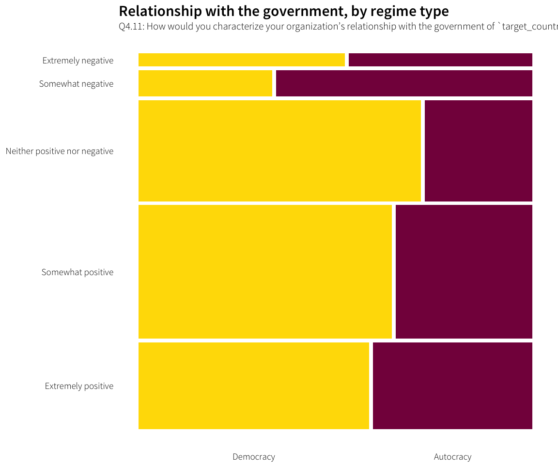
govt.positivity.regime.table <- survey.countries.clean %>%
  filter(Q4.11 != "Don't know", Q4.11 != "Prefer not to answer") %>%
  mutate(Q4.11 = droplevels(Q4.11)) %>%
  xtabs(~ Q4.11 + target.regime.type, .)

analyze.cat.var(govt.positivity.regime.table)
## Table counts
## target.regime.type Democracy Autocracy
## Q4.11
## Extremely negative 9 8
## Somewhat negative 12 23
## Neither positive nor negative 97 37
## Somewhat positive 115 62
## Extremely positive 68 47
##
## Expected values
## target.regime.type
## Q4.11 Democracy Autocracy
## Extremely negative 10.70502 6.294979
## Somewhat negative 22.03975 12.960251
## Neither positive nor negative 84.38075 49.619247
## Somewhat positive 111.45816 65.541841
## Extremely positive 72.41632 42.583682
##
## Row proporitions
## target.regime.type Democracy Autocracy
## Q4.11
## Extremely negative 0.5294118 0.4705882
## Somewhat negative 0.3428571 0.6571429
## Neither positive nor negative 0.7238806 0.2761194
## Somewhat positive 0.6497175 0.3502825
## Extremely positive 0.5913043 0.4086957
##
## Column proporitions
## target.regime.type Democracy Autocracy
## Q4.11
## Extremely negative 0.02990033 0.04519774
## Somewhat negative 0.03986711 0.12994350
## Neither positive nor negative 0.32225914 0.20903955
## Somewhat positive 0.38205980 0.35028249
## Extremely positive 0.22591362 0.26553672
##
## Chi-squared test for table
##
## Pearson's Chi-squared test
##
## data: ftable(cat.table)
## X-squared = 19.212, df = 4, p-value = 0.000714
##
## Cramer's V
## [1] 0.2004806
##
## Pearson residuals
## 2 is used as critical value by convention
## target.regime.type Democracy Autocracy
## Q4.11
## Extremely negative -0.5211179 0.6795674
## Somewhat negative -2.1385506 2.7887921
## Neither positive nor negative 1.3737628 -1.7914651
## Somewhat positive 0.3354850 -0.4374916
## Extremely positive -0.5189698 0.6767663
##
## Components of chi-squared
## Critical value (0.05 with 4 df) is 9.49
## target.regime.type Democracy Autocracy
## Q4.11
## Extremely negative 0.2715638 0.4618119
## Somewhat negative 4.5733987 7.7773616
## Neither positive nor negative 1.8872241 3.2093472
## Somewhat positive 0.1125502 0.1913989
## Extremely positive 0.2693297 0.4580126
##
## p for components
## target.regime.type Democracy Autocracy
## Q4.11
## Extremely negative 0.992 0.977
## Somewhat negative 0.334 0.100
## Neither positive nor negative 0.756 0.523
## Somewhat positive 0.998 0.996
## Extremely positive 0.992 0.977NGO regulations and restrictions
Familiarity
Most INGOs working in democracies are either moderately familiar with government regulations or not familiar at all. For INGOs working in autocracies, familiarity with regulations appears to be more essential—most are very or extremely familiar with regulations, and very few are unaware of any of the laws governing their activities. The difference in proporitions across groups is significant.
df.reg.familiarity.regime <- survey.countries.clean %>%
  select(Q4.13, target.regime.type) %>%
  filter(!is.na(Q4.13))

plot.reg.familiarity.regime <- prodplot(df.reg.familiarity.regime,
                                        ~ target.regime.type + Q4.13, mosaic("h"),
                                        colour=NA) +
  aes(fill=target.regime.type, colour="white") +
  scale_fill_manual(values=ath.palette("regime"), name=NULL) +
  guides(fill=FALSE) +
  labs(title="Familiarity with regulations, by regime type",
       subtitle="Q4.13: How familiar is your organization with regulations for\ninternational nongovernmental organizations (NGOs) in `target_country`?") +
  theme_ath() + theme(axis.title=element_blank(),
                      panel.grid=element_blank())
plot.reg.familiarity.regime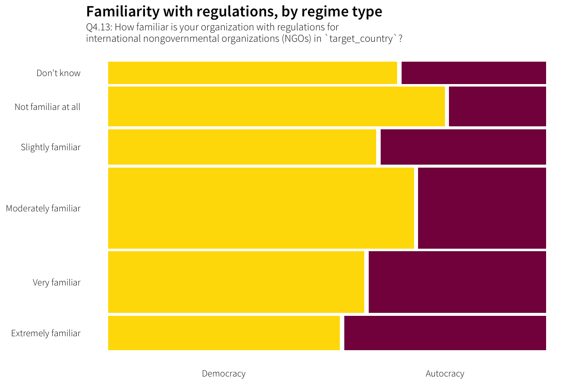
reg.familiarity.regime.table <- survey.countries.clean %>%
  xtabs(~ Q4.13 + target.regime.type, .)

analyze.cat.var(reg.familiarity.regime.table)
## Table counts
## target.regime.type Democracy Autocracy
## Q4.13
## Extremely familiar 39 34
## Very familiar 78 54
## Moderately familiar 122 51
## Slightly familiar 47 29
## Not familiar at all 66 19
## Don't know 32 16
##
## Expected values
## target.regime.type
## Q4.13 Democracy Autocracy
## Extremely familiar 47.75468 25.24532
## Very familiar 86.35094 45.64906
## Moderately familiar 113.17206 59.82794
## Slightly familiar 49.71721 26.28279
## Not familiar at all 55.60477 29.39523
## Don't know 31.40034 16.59966
##
## Row proporitions
## target.regime.type Democracy Autocracy
## Q4.13
## Extremely familiar 0.5342466 0.4657534
## Very familiar 0.5909091 0.4090909
## Moderately familiar 0.7052023 0.2947977
## Slightly familiar 0.6184211 0.3815789
## Not familiar at all 0.7764706 0.2235294
## Don't know 0.6666667 0.3333333
##
## Column proporitions
## target.regime.type Democracy Autocracy
## Q4.13
## Extremely familiar 0.10156250 0.16748768
## Very familiar 0.20312500 0.26600985
## Moderately familiar 0.31770833 0.25123153
## Slightly familiar 0.12239583 0.14285714
## Not familiar at all 0.17187500 0.09359606
## Don't know 0.08333333 0.07881773
##
## Chi-squared test for table
##
## Pearson's Chi-squared test
##
## data: ftable(cat.table)
## X-squared = 15.05, df = 5, p-value = 0.01015
##
## Cramer's V
## [1] 0.1601189
##
## Pearson residuals
## 2 is used as critical value by convention
## target.regime.type Democracy Autocracy
## Q4.13
## Extremely familiar -1.2668714 1.7424090
## Very familiar -0.8986730 1.2360023
## Moderately familiar 0.8298311 -1.1413196
## Slightly familiar -0.3853623 0.5300134
## Not familiar at all 1.3940491 -1.9173247
## Don't know 0.1070132 -0.1471821
##
## Components of chi-squared
## Critical value (0.05 with 5 df) is 11.07
## target.regime.type Democracy Autocracy
## Q4.13
## Extremely familiar 1.60496309 3.03598930
## Very familiar 0.80761310 1.52770164
## Moderately familiar 0.68861961 1.30261050
## Slightly familiar 0.14850410 0.28091417
## Not familiar at all 1.94337296 3.67613407
## Don't know 0.01145183 0.02166257
##
## p for components
## target.regime.type Democracy Autocracy
## Q4.13
## Extremely familiar 0.901 0.694
## Very familiar 0.977 0.910
## Moderately familiar 0.984 0.935
## Slightly familiar 1.000 0.998
## Not familiar at all 0.857 0.597
## Don't know 1.000 1.000Frequency of change
freq.change.collapsed <- c("Once a year+", "Once every few years",
                           "Rarely or never", "Don't know")

df.freq.change <- survey.countries.clean %>%
  filter(!is.na(Q4.14)) %>%
  mutate(Q4.14.collapsed = case_when(
    .$Q4.14 == "Once a month" ~ freq.change.collapsed[1],
    .$Q4.14 == "Once a year" ~ freq.change.collapsed[1],
    .$Q4.14 == "Once every few years" ~ freq.change.collapsed[2],
    .$Q4.14 == "Rarely" ~ freq.change.collapsed[3],
    .$Q4.14 == "Never" ~ freq.change.collapsed[3],
    .$Q4.14 == "Don't know" ~ freq.change.collapsed[4],
    TRUE ~ NA_character_)) %>%
  filter(!is.na(Q4.14.collapsed)) %>%
  mutate(Q4.14.collapsed = factor(Q4.14.collapsed, levels=rev(freq.change.collapsed),
                                  ordered=TRUE))
Regime type
Most NGOs don’t know, and I didn’t include an “other” category here. The univariate distribution has a clear trend, with most reporting “Rarely” (and only a few “Never”; “Never” and “Once a month” are collapsed because of low expected values). There’s also a trend by regime type—more INGOs working in autocracies see annual changes in regulations, possibly reflecting a more volatile regulatory environment.
plot.reg.change.regime <- prodplot(df.freq.change,
                                        ~ target.regime.type + Q4.14.collapsed, mosaic("h"),
                                        colour=NA) +
  aes(fill=target.regime.type, colour="white") +
  scale_fill_manual(values=ath.palette("regime"), name=NULL) +
  guides(fill=FALSE) +
  labs(title="Frequency of changes, by regime type",
       subtitle="Q4.14: How often do regulations for international NGOs in `target_country` change?") +
  theme_ath() + theme(axis.title=element_blank(),
                      panel.grid=element_blank())
plot.reg.change.regime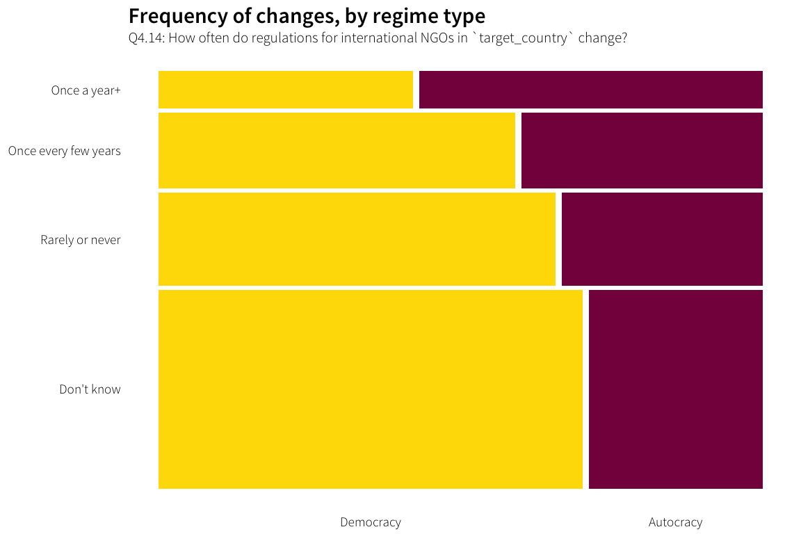
reg.change.regime.table <- df.freq.change %>%
  xtabs(~ Q4.14.collapsed + target.regime.type, .)

analyze.cat.var(reg.change.regime.table)
## Table counts
## target.regime.type Democracy Autocracy
## Q4.14.collapsed
## Don't know 203 83
## Rarely or never 89 45
## Once every few years 65 44
## Once a year+ 23 31
##
## Expected values
## target.regime.type
## Q4.14.collapsed Democracy Autocracy
## Don't know 186.41509 99.58491
## Rarely or never 87.34134 46.65866
## Once every few years 71.04631 37.95369
## Once a year+ 35.19726 18.80274
##
## Row proporitions
## target.regime.type Democracy Autocracy
## Q4.14.collapsed
## Don't know 0.7097902 0.2902098
## Rarely or never 0.6641791 0.3358209
## Once every few years 0.5963303 0.4036697
## Once a year+ 0.4259259 0.5740741
##
## Column proporitions
## target.regime.type Democracy Autocracy
## Q4.14.collapsed
## Don't know 0.53421053 0.40886700
## Rarely or never 0.23421053 0.22167488
## Once every few years 0.17105263 0.21674877
## Once a year+ 0.06052632 0.15270936
##
## Chi-squared test for table
##
## Pearson's Chi-squared test
##
## data: ftable(cat.table)
## X-squared = 17.945, df = 3, p-value = 0.0004515
##
## Cramer's V
## [1] 0.1754434
##
## Pearson residuals
## 2 is used as critical value by convention
## target.regime.type Democracy Autocracy
## Q4.14.collapsed
## Don't know 1.2147096 -1.6619435
## Rarely or never 0.1774794 -0.2428241
## Once every few years -0.7173313 0.9814396
## Once a year+ -2.0559272 2.8128819
##
## Components of chi-squared
## Critical value (0.05 with 3 df) is 7.81
## target.regime.type Democracy Autocracy
## Q4.14.collapsed
## Don't know 1.47551944 2.76205610
## Rarely or never 0.03149894 0.05896354
## Once every few years 0.51456423 0.96322368
## Once a year+ 4.22683647 7.91230472
##
## p for components
## target.regime.type Democracy Autocracy
## Q4.14.collapsed
## Don't know 0.688 0.430
## Rarely or never 0.999 0.996
## Once every few years 0.916 0.810
## Once a year+ 0.238 0.048Potential contentiousness
There’s no difference in the frequency of changes across issue areas, which is to be expected. Actual legal restrictions are a blunt instrument and don’t really target specific sectors of INGOs.
plot.reg.change.issue <- prodplot(df.freq.change,
                                  ~ potential.contentiousness + Q4.14.collapsed, mosaic("h"),
                                  colour=NA) +
  aes(fill=potential.contentiousness, colour="white") +
  scale_fill_manual(values=ath.palette("contention"), name=NULL) +
  guides(fill=FALSE) +
  labs(title="Frequency of changes, by issue",
       subtitle="Q4.14: How often do regulations for international NGOs in `target_country` change?") +
  theme_ath() + theme(axis.title=element_blank(),
                      panel.grid=element_blank())
plot.reg.change.issue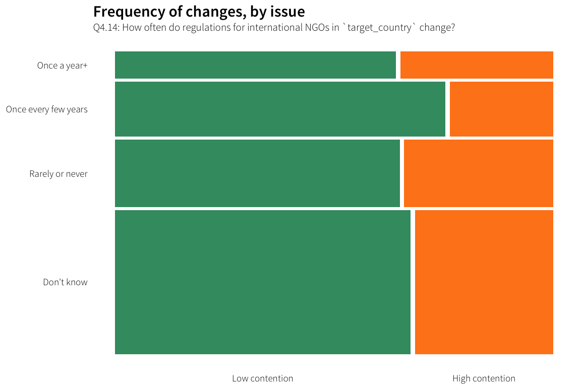
reg.change.issue.table <- df.freq.change %>%
  xtabs(~ Q4.14.collapsed + potential.contentiousness, .)

analyze.cat.var(reg.change.issue.table)
## Table counts
## potential.contentiousness Low contention High contention
## Q4.14.collapsed
## Don't know 195 91
## Rarely or never 88 46
## Once every few years 83 26
## Once a year+ 35 19
##
## Expected values
## potential.contentiousness
## Q4.14.collapsed Low contention High contention
## Don't know 196.71698 89.28302
## Rarely or never 92.16810 41.83190
## Once every few years 74.97256 34.02744
## Once a year+ 37.14237 16.85763
##
## Row proporitions
## potential.contentiousness Low contention High contention
## Q4.14.collapsed
## Don't know 0.6818182 0.3181818
## Rarely or never 0.6567164 0.3432836
## Once every few years 0.7614679 0.2385321
## Once a year+ 0.6481481 0.3518519
##
## Column proporitions
## potential.contentiousness Low contention High contention
## Q4.14.collapsed
## Don't know 0.4862843 0.5000000
## Rarely or never 0.2194514 0.2527473
## Once every few years 0.2069825 0.1428571
## Once a year+ 0.0872818 0.1043956
##
## Chi-squared test for table
##
## Pearson's Chi-squared test
##
## data: ftable(cat.table)
## X-squared = 3.8009, df = 3, p-value = 0.2838
##
## Cramer's V
## [1] 0.0807439
##
## Pearson residuals
## 2 is used as critical value by convention
## potential.contentiousness Low contention High contention
## Q4.14.collapsed
## Don't know -0.1224178 0.1817109
## Rarely or never -0.4341576 0.6444421
## Once every few years 0.9270991 -1.3761400
## Once a year+ -0.3515273 0.5217898
##
## Components of chi-squared
## Critical value (0.05 with 3 df) is 7.81
## potential.contentiousness Low contention High contention
## Q4.14.collapsed
## Don't know 0.01498612 0.03301887
## Rarely or never 0.18849282 0.41530562
## Once every few years 0.85951267 1.89376142
## Once a year+ 0.12357146 0.27226460
##
## p for components
## potential.contentiousness Low contention High contention
## Q4.14.collapsed
## Don't know 1.000 0.998
## Rarely or never 0.979 0.937
## Once every few years 0.835 0.595
## Once a year+ 0.989 0.965How do they find out about changes?
INGOs working in different regimes hear about changes somewhat differently as well. Those working in autocracies are more likely to hear about changes in regulations directly from government officials, while those in demcoracies are way less likely to do so. Other NGOs are the most common source for both regime types, and all other categories are in the same order and roughly the same proportion. This makes sense since INGOs already have more regular contact with government officials in autocracies.
df.change.how.regime <- survey.countries.clean %>%
  unnest(Q4.15_value) %>%
  select(Q4.15 = Q4.15_value, target.regime.type) %>%
  filter(Q4.15 != "Don't know") %>%
  mutate(Q4.15 = factor(Q4.15))

levels(df.change.how.regime$Q4.15)[levels(df.change.how.regime$Q4.15) == "Newspapers, television, and other media"] <-
  "Newspapers, television,\nand other media"

plot.change.how.regime <- prodplot(df.change.how.regime,
                                   ~ target.regime.type + Q4.15, mosaic("h"),
                                   colour=NA) +
  aes(fill=target.regime.type, colour="white") +
  scale_fill_manual(values=ath.palette("regime"), name=NULL) +
  guides(fill=FALSE) +
  labs(title="How NGOs find out, by regime type",
       subtitle="Q4.15: How does your organization find out about changes to\nNGO regulations in `target_country`? (multiple answers allowed)") +
  theme_ath() + theme(axis.title=element_blank(),
                      panel.grid=element_blank())
plot.change.how.regime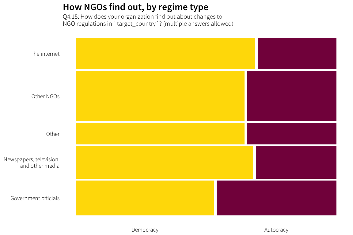
plot.df.change.how.regime <- df.change.how.regime %>%
  group_by(target.regime.type, Q4.15) %>%
  summarise(num = n()) %>%
  mutate(perc = num / sum(num)) %>%
  arrange(perc) %>%
  ungroup() %>%
  mutate(Q4.15 = factor(Q4.15, levels=unique(Q4.15), ordered=TRUE))

plot.change.how.regime.bar <- ggplot(plot.df.change.how.regime,
                                     aes(x=perc, y=Q4.15,
                                         fill=target.regime.type)) +
  geom_barh(stat="identity") +
  scale_fill_manual(values=ath.palette("regime"), name=NULL) +
  scale_x_continuous(labels=percent) +
  labs(x=NULL, y=NULL, title="Percentages by regime type") +
  guides(fill=FALSE) +
  theme_ath() +
  facet_wrap(~ target.regime.type)
plot.change.how.regime.bar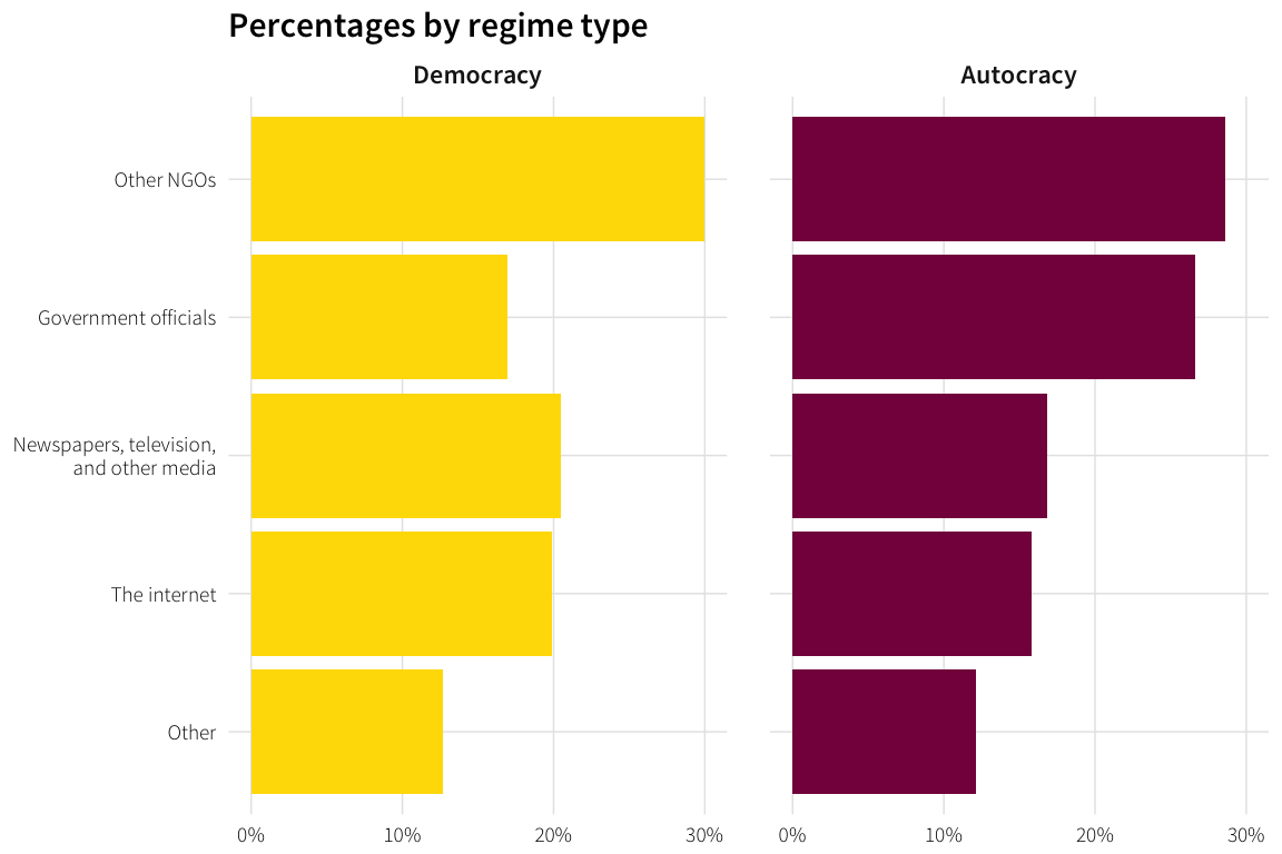
change.how.table <- survey.countries.clean %>%
  unnest(Q4.15_value) %>%
  filter(Q4.15_value != "Don't know") %>%
  xtabs(~ Q4.15_value + target.regime.type, .)

analyze.cat.var(change.how.table)
## Table counts
## target.regime.type Democracy Autocracy
## Q4.15_value
## Government officials 91 79
## Newspapers, television, and other media 110 50
## Other 68 36
## Other NGOs 161 85
## The internet 107 47
##
## Expected values
## target.regime.type
## Q4.15_value Democracy Autocracy
## Government officials 109.46043 60.53957
## Newspapers, television, and other media 103.02158 56.97842
## Other 66.96403 37.03597
## Other NGOs 158.39568 87.60432
## The internet 99.15827 54.84173
##
## Row proporitions
## target.regime.type Democracy Autocracy
## Q4.15_value
## Government officials 0.5352941 0.4647059
## Newspapers, television, and other media 0.6875000 0.3125000
## Other 0.6538462 0.3461538
## Other NGOs 0.6544715 0.3455285
## The internet 0.6948052 0.3051948
##
## Column proporitions
## target.regime.type Democracy Autocracy
## Q4.15_value
## Government officials 0.1694600 0.2659933
## Newspapers, television, and other media 0.2048417 0.1683502
## Other 0.1266294 0.1212121
## Other NGOs 0.2998138 0.2861953
## The internet 0.1992551 0.1582492
##
## Chi-squared test for table
##
## Pearson's Chi-squared test
##
## data: ftable(cat.table)
## X-squared = 11.977, df = 4, p-value = 0.01753
##
## Cramer's V
## [1] 0.1198348
##
## Pearson residuals
## 2 is used as critical value by convention
## target.regime.type Democracy Autocracy
## Q4.15_value
## Government officials -1.7644659 2.3725872
## Newspapers, television, and other media 0.6875319 -0.9244890
## Other 0.1265980 -0.1702299
## Other NGOs 0.2069294 -0.2782473
## The internet 0.7874939 -1.0589029
##
## Components of chi-squared
## Critical value (0.05 with 4 df) is 9.49
## target.regime.type Democracy Autocracy
## Q4.15_value
## Government officials 3.11333997 5.62917025
## Newspapers, television, and other media 0.47270005 0.85467989
## Other 0.01602706 0.02897822
## Other NGOs 0.04281976 0.07742158
## The internet 0.62014670 1.12127535
##
## p for components
## target.regime.type Democracy Autocracy
## Q4.15_value
## Government officials 0.539 0.229
## Newspapers, television, and other media 0.976 0.931
## Other 1.000 1.000
## Other NGOs 1.000 0.999
## The internet 0.961 0.891Effect of regulations
TODO: Do this
Effect of regulations in general
Regime type
!!! It works !!!
INGOs that are restricted tend to work in autocracies and there’s almost a perfect trend.
df.reg.effect.general.regime <- survey.countries.clean %>%
  select(Q4.17, target.regime.type) %>%
  filter(Q4.17 != "Don’t know") %>%
  mutate(Q4.17 = droplevels(Q4.17),
         Q4.17 = factor(Q4.17, levels=rev(levels(Q4.17))))

plot.reg.effect.general.regime <- prodplot(df.reg.effect.general.regime,
                                   ~ target.regime.type + Q4.17, mosaic("h"),
                                   colour=NA) +
  aes(fill=target.regime.type, colour="white") +
  scale_fill_manual(values=ath.palette("regime"), name=NULL) +
  guides(fill=FALSE) +
  labs(title="General restrictions, by regime type",
       subtitle="Q4.17: Overall, how is your organization's work affected by government regulations in `target_country`?") +
  theme_ath() + theme(axis.title=element_blank(),
                      panel.grid=element_blank())
plot.reg.effect.general.regime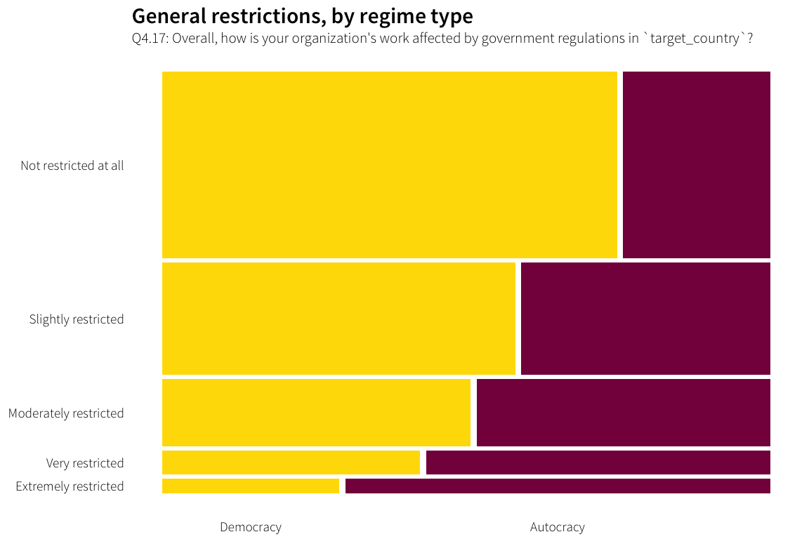
reg.effect.general.regime.table <- survey.countries.clean %>%
  xtabs(~ Q4.17 + target.regime.type, .)

analyze.cat.var(reg.effect.general.regime.table)
## Table counts
## target.regime.type Democracy Autocracy
## Q4.17
## Not restricted at all 167 54
## Slightly restricted 78 55
## Moderately restricted 41 39
## Very restricted 12 16
## Extremely restricted 5 12
## Don’t know 56 17
##
## Expected values
## target.regime.type
## Q4.17 Democracy Autocracy
## Not restricted at all 143.73007 77.269928
## Slightly restricted 86.49819 46.501812
## Moderately restricted 52.02899 27.971014
## Very restricted 18.21014 9.789855
## Extremely restricted 11.05616 5.943841
## Don’t know 47.47645 25.523551
##
## Row proporitions
## target.regime.type Democracy Autocracy
## Q4.17
## Not restricted at all 0.7556561 0.2443439
## Slightly restricted 0.5864662 0.4135338
## Moderately restricted 0.5125000 0.4875000
## Very restricted 0.4285714 0.5714286
## Extremely restricted 0.2941176 0.7058824
## Don’t know 0.7671233 0.2328767
##
## Column proporitions
## target.regime.type Democracy Autocracy
## Q4.17
## Not restricted at all 0.46518106 0.27979275
## Slightly restricted 0.21727019 0.28497409
## Moderately restricted 0.11420613 0.20207254
## Very restricted 0.03342618 0.08290155
## Extremely restricted 0.01392758 0.06217617
## Don’t know 0.15598886 0.08808290
##
## Chi-squared test for table
##
## Pearson's Chi-squared test
##
## data: ftable(cat.table)
## X-squared = 39.772, df = 5, p-value = 1.66e-07
##
## Cramer's V
## [1] 0.2684213
##
## Pearson residuals
## 2 is used as critical value by convention
## target.regime.type Democracy Autocracy
## Q4.17
## Not restricted at all 1.9409807 -2.6472184
## Slightly restricted -0.9137404 1.2462105
## Moderately restricted -1.5290190 2.0853620
## Very restricted -1.4552749 1.9847856
## Extremely restricted -1.8213573 2.4840694
## Don’t know 1.2370334 -1.6871357
##
## Components of chi-squared
## Critical value (0.05 with 5 df) is 11.07
## target.regime.type Democracy Autocracy
## Q4.17
## Not restricted at all 3.7674059 7.0077654
## Slightly restricted 0.8349216 1.5530407
## Moderately restricted 2.3378992 4.3487347
## Very restricted 2.1178250 3.9393739
## Extremely restricted 3.3173424 6.1706007
## Don’t know 1.5302517 2.8464267
##
## p for components
## target.regime.type Democracy Autocracy
## Q4.17
## Not restricted at all 0.583 0.220
## Slightly restricted 0.975 0.907
## Moderately restricted 0.801 0.500
## Very restricted 0.833 0.558
## Extremely restricted 0.651 0.290
## Don’t know 0.910 0.724Potential contentiousness
Differences in general restrictions by issue are less pronounced. There is a significant overall difference, driven primarily by high contention INGOs that report feeling extremely restricted. All levels of restriction are relatively even, following a 65-35 split between low and high contention INGOs.
df.reg.effect.general.issue <- survey.countries.clean %>%
  select(Q4.17, potential.contentiousness) %>%
  filter(Q4.17 != "Don’t know") %>%
  mutate(Q4.17 = droplevels(Q4.17),
         Q4.17 = factor(Q4.17, levels=rev(levels(Q4.17))))

plot.reg.effect.general.issue <- prodplot(df.reg.effect.general.issue,
                                          ~ potential.contentiousness + Q4.17, mosaic("h"),
                                          colour=NA) +
  aes(fill=potential.contentiousness, colour="white") +
  scale_fill_manual(values=ath.palette("contention"), name=NULL) +
  guides(fill=FALSE) +
  labs(title="General restrictions, by issue",
       subtitle="Q4.17: Overall, how is your organization's work affected by government regulations in `target_country`?") +
  theme_ath() + theme(axis.title=element_blank(),
                      panel.grid=element_blank())
plot.reg.effect.general.issue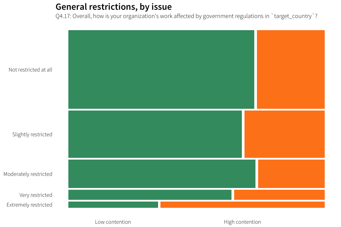
reg.effect.general.issue.table <- survey.countries.clean %>%
  xtabs(~ Q4.17 + potential.contentiousness, .)

analyze.cat.var(reg.effect.general.issue.table)
## Table counts
## potential.contentiousness Low contention High contention
## Q4.17
## Not restricted at all 162 59
## Slightly restricted 91 42
## Moderately restricted 59 21
## Very restricted 18 10
## Extremely restricted 6 11
## Don’t know 47 26
##
## Expected values
## potential.contentiousness
## Q4.17 Low contention High contention
## Not restricted at all 153.33877 67.661232
## Slightly restricted 92.28080 40.719203
## Moderately restricted 55.50725 24.492754
## Very restricted 19.42754 8.572464
## Extremely restricted 11.79529 5.204710
## Don’t know 50.65036 22.349638
##
## Row proporitions
## potential.contentiousness Low contention High contention
## Q4.17
## Not restricted at all 0.7330317 0.2669683
## Slightly restricted 0.6842105 0.3157895
## Moderately restricted 0.7375000 0.2625000
## Very restricted 0.6428571 0.3571429
## Extremely restricted 0.3529412 0.6470588
## Don’t know 0.6438356 0.3561644
##
## Column proporitions
## potential.contentiousness Low contention High contention
## Q4.17
## Not restricted at all 0.42297650 0.34911243
## Slightly restricted 0.23759791 0.24852071
## Moderately restricted 0.15404700 0.12426036
## Very restricted 0.04699739 0.05917160
## Extremely restricted 0.01566580 0.06508876
## Don’t know 0.12271540 0.15384615
##
## Chi-squared test for table
##
## Pearson's Chi-squared test
##
## data: ftable(cat.table)
## X-squared = 12.876, df = 5, p-value = 0.02457
##
## Cramer's V
## [1] 0.1527288
##
## Pearson residuals
## 2 is used as critical value by convention
## potential.contentiousness Low contention High contention
## Q4.17
## Not restricted at all 0.6994452 -1.0529548
## Slightly restricted -0.1333290 0.2007154
## Moderately restricted 0.4688059 -0.7057472
## Very restricted -0.3238756 0.4875670
## Extremely restricted -1.6874109 2.5402525
## Don’t know -0.5129142 0.7721483
##
## Components of chi-squared
## Critical value (0.05 with 5 df) is 11.07
## potential.contentiousness Low contention High contention
## Q4.17
## Not restricted at all 0.48922356 1.10871374
## Slightly restricted 0.01777663 0.04028667
## Moderately restricted 0.21977901 0.49807907
## Very restricted 0.10489543 0.23772159
## Extremely restricted 2.84735559 6.45288279
## Don’t know 0.26308094 0.59621302
##
## p for components
## potential.contentiousness Low contention High contention
## Q4.17
## Not restricted at all 0.993 0.953
## Slightly restricted 1.000 1.000
## Moderately restricted 0.999 0.992
## Very restricted 1.000 0.999
## Extremely restricted 0.724 0.265
## Don’t know 0.998 0.988Regime type + contentiousness
There are more unrestricted low contentious NGOs working in democracies than expected and far fewer unrestricted low contentious NGOs in autocracies. Additionally, there are fewer highly restricted INGOs in democracies (especially high contentious ones), and far more highly restricted, highly contentious INGOs working in autocracies than expected.
# Collapse very and extremely restriced because of low expected frequencies
restricted <- c("Not restricted at all", "Slightly restricted",
                "Moderately restricted", "Very or extremely restricted")

df.reg.effect.general.issue.regime <- survey.countries.clean %>%
  select(Q4.17, potential.contentiousness, target.regime.type) %>%
  filter(Q4.17 != "Don’t know") %>%
  mutate(Q4.17 = recode_factor(Q4.17, `Very restricted` = restricted[4],
                        `Extremely restricted` = restricted[4]),
         Q4.17 = factor(Q4.17, levels=restricted, ordered=TRUE))

plot.reg.effect.general.issue.regime <- prodplot(df.reg.effect.general.issue.regime,
                                          ~ target.regime.type + potential.contentiousness +
                                            Q4.17, mosaic("v")) +
  aes(fill=target.regime.type, linetype=potential.contentiousness) +
  scale_fill_manual(values=ath.palette("regime")) +
  scale_linetype_manual(values=c("blank", "dashed")) +
  guides(fill=FALSE, linetype=FALSE) +
  labs(title="General restrictions, by issue and regime type",
       subtitle="Q4.17: Overall, how is your organization's work affected by government regulations in `target_country`?") +
  theme_ath() + theme(axis.title=element_blank(),
                      panel.grid=element_blank())
plot.reg.effect.general.issue.regime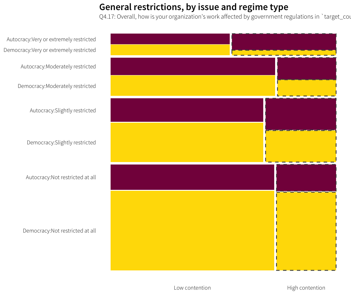
reg.effect.general.regime.issue.table <- df.reg.effect.general.issue.regime %>%
  xtabs(~ Q4.17 + potential.contentiousness + target.regime.type, .)

analyze.cat.var(reg.effect.general.regime.issue.table)
## Table counts
## target.regime.type Democracy Autocracy
## Q4.17 potential.contentiousness
## Not restricted at all Low contention 123 39
## High contention 44 15
## Slightly restricted Low contention 57 34
## High contention 21 21
## Moderately restricted Low contention 32 27
## High contention 9 12
## Very or extremely restricted Low contention 12 12
## High contention 5 16
##
## Expected values
## [,1] [,2]
## [1,] 102.47599 59.524008
## [2,] 37.32150 21.678497
## [3,] 57.56367 33.436326
## [4,] 26.56785 15.432150
## [5,] 37.32150 21.678497
## [6,] 13.28392 7.716075
## [7,] 15.18163 8.818372
## [8,] 13.28392 7.716075
##
## Row proporitions
## target.regime.type Democracy Autocracy
## Q4.17 potential.contentiousness
## Not restricted at all Low contention 0.5565611 0.1764706
## High contention 0.1990950 0.0678733
## Slightly restricted Low contention 0.4285714 0.2556391
## High contention 0.1578947 0.1578947
## Moderately restricted Low contention 0.4000000 0.3375000
## High contention 0.1125000 0.1500000
## Very or extremely restricted Low contention 0.2666667 0.2666667
## High contention 0.1111111 0.3555556
##
## Column proporitions
## target.regime.type Democracy Autocracy
## Q4.17 potential.contentiousness
## Not restricted at all Low contention 0.36607143 0.11607143
## High contention 0.30769231 0.10489510
## Slightly restricted Low contention 0.16964286 0.10119048
## High contention 0.14685315 0.14685315
## Moderately restricted Low contention 0.09523810 0.08035714
## High contention 0.06293706 0.08391608
## Very or extremely restricted Low contention 0.03571429 0.03571429
## High contention 0.03496503 0.11188811
##
## Chi-squared test for table
##
## Pearson's Chi-squared test
##
## data: ftable(cat.table)
## X-squared = 39.33, df = 7, p-value = 1.691e-06
##
## Cramer's V
## [1] 0.2865449
##
## Pearson residuals
## 2 is used as critical value by convention
## target.regime.type Democracy Autocracy
## Q4.17 potential.contentiousness
## Not restricted at all Low contention 2.02745451 -2.66021108
## High contention 1.09319884 -1.43437974
## Slightly restricted Low contention -0.07429404 0.09748078
## High contention -1.08021275 1.41734077
## Moderately restricted Low contention -0.87107341 1.14293028
## High contention -1.17538092 1.54221037
## Very or extremely restricted Low contention -0.81656409 1.07140891
## High contention -2.27286136 2.98220796
##
## Components of chi-squared
## Critical value (0.05 with 7 df) is 14.07
## target.regime.type Democracy Autocracy
## Q4.17 potential.contentiousness
## Not restricted at all Low contention 4.110571774 7.076722997
## High contention 1.195083710 2.057445251
## Slightly restricted Low contention 0.005519605 0.009502502
## High contention 1.166859588 2.008854859
## Moderately restricted Low contention 0.758768892 1.306289627
## High contention 1.381520317 2.378412819
## Very or extremely restricted Low contention 0.666776907 1.147917062
## High contention 5.165898755 8.893564334
##
## p for components
## target.regime.type Democracy Autocracy
## Q4.17 potential.contentiousness
## Not restricted at all Low contention 0.767 0.421
## High contention 0.991 0.957
## Slightly restricted Low contention 1.000 1.000
## High contention 0.992 0.959
## Moderately restricted Low contention 0.998 0.988
## High contention 0.986 0.936
## Very or extremely restricted Low contention 0.999 0.992
## High contention 0.640 0.260Responses to regulations
Changes in programming
Regime type
Slightly more NGOs that work in autocracies have changed their programming in the past decade, but not in a statistically significant way. In general, most INGOs have not changed much, and the split is proportional across regime type.
df.change.programming.regime <- survey.countries.clean %>%
  filter(!is.na(Q4.19)) %>%
  filter(Q4.19 != "Don't know") %>%
  mutate(Q4.19 = droplevels(Q4.19),
         Q4.19 = factor(Q4.19, levels=rev(levels(Q4.19)))) %>%
  select(Q4.19, target.regime.type)

plot.change.programming.regime <- prodplot(df.change.programming.regime,
                                    ~ target.regime.type + Q4.19, mosaic("h"),
                                    colour=NA) +
  aes(fill=target.regime.type, colour="white") +
  scale_fill_manual(values=ath.palette("regime"), name=NULL) +
  guides(fill=FALSE) +
  labs(title="Change in programming, by regime type",
       subtitle="Q4.19: Over the last 10 years, has your organization changed its mix of programming in `target_country`?") +
  theme_ath() + theme(axis.title=element_blank(),
                      panel.grid=element_blank())
plot.change.programming.regime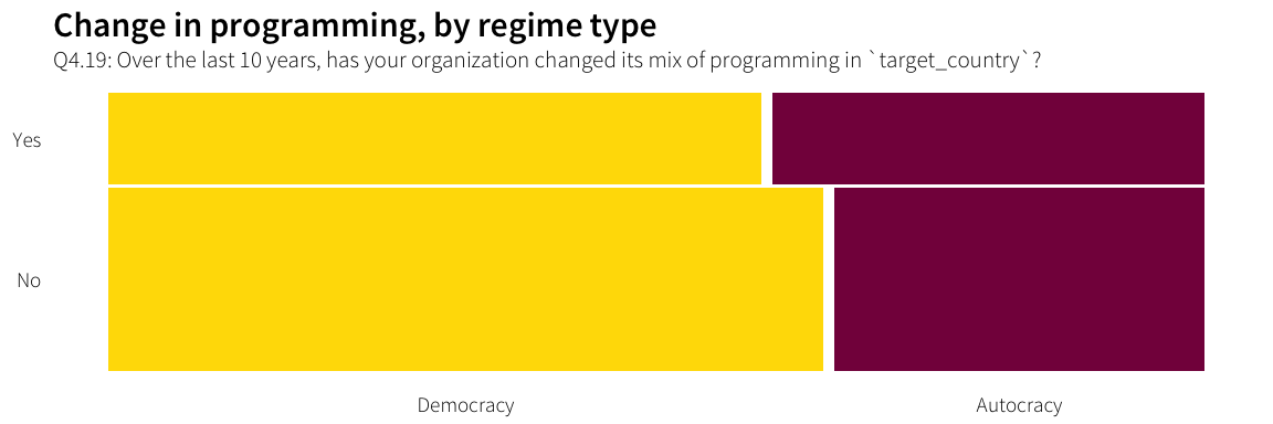
change.programming.table <- df.change.programming.regime %>%
  xtabs(~ Q4.19 + target.regime.type, .)

analyze.cat.var(change.programming.table)
## Table counts
## target.regime.type Democracy Autocracy
## Q4.19
## No 222 115
## Yes 101 67
##
## Expected values
## target.regime.type
## Q4.19 Democracy Autocracy
## No 215.5465 121.45347
## Yes 107.4535 60.54653
##
## Row proporitions
## target.regime.type Democracy Autocracy
## Q4.19
## No 0.6587537 0.3412463
## Yes 0.6011905 0.3988095
##
## Column proporitions
## target.regime.type Democracy Autocracy
## Q4.19
## No 0.6873065 0.6318681
## Yes 0.3126935 0.3681319
##
## Chi-squared test for table
##
## Pearson's Chi-squared test with Yates' continuity correction
##
## data: ftable(cat.table)
## X-squared = 1.3715, df = 1, p-value = 0.2416
##
## Cramer's V
## [1] 0.05649081
##
## Pearson residuals
## 2 is used as critical value by convention
## target.regime.type Democracy Autocracy
## Q4.19
## No 0.4395643 -0.5855824
## Yes -0.6225622 0.8293700
##
## Components of chi-squared
## Critical value (0.05 with 1 df) is 3.84
## target.regime.type Democracy Autocracy
## Q4.19
## No 0.1932168 0.3429068
## Yes 0.3875837 0.6878546
##
## p for components
## target.regime.type Democracy Autocracy
## Q4.19
## No 0.660 0.558
## Yes 0.534 0.407Potential contentiousness
Slightly fewer INGOs working on highly contentious issues have changed their programming over the past decade, but again, the difference between expected and actual is not significant.
df.change.programming.issue <- survey.countries.clean %>%
  filter(!is.na(Q4.19)) %>%
  filter(Q4.19 != "Don't know") %>%
  mutate(Q4.19 = droplevels(Q4.19),
         Q4.19 = factor(Q4.19, levels=rev(levels(Q4.19)))) %>%
  select(Q4.19, potential.contentiousness)

plot.change.programming.issue <- prodplot(df.change.programming.issue,
                                   ~ potential.contentiousness + Q4.19, mosaic("h"),
                                   colour=NA) +
  aes(fill=potential.contentiousness, colour="white") +
  scale_fill_manual(values=ath.palette("contention"), name=NULL) +
  guides(fill=FALSE) +
  labs(title="Change in programming, by issue",
       subtitle="Q4.19: Over the last 10 years, has your organization changed its mix of programming in `target_country`?") +
  theme_ath() + theme(axis.title=element_blank(),
                      panel.grid=element_blank())
plot.change.programming.issue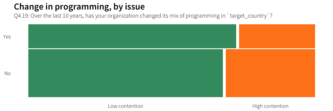
change.programming.issue.table <- df.change.programming.issue %>%
  xtabs(~ Q4.19 + potential.contentiousness, .)

analyze.cat.var(change.programming.issue.table)
## Table counts
## potential.contentiousness Low contention High contention
## Q4.19
## No 231 106
## Yes 123 45
##
## Expected values
## potential.contentiousness
## Q4.19 Low contention High contention
## No 236.2337 100.76634
## Yes 117.7663 50.23366
##
## Row proporitions
## potential.contentiousness Low contention High contention
## Q4.19
## No 0.6854599 0.3145401
## Yes 0.7321429 0.2678571
##
## Column proporitions
## potential.contentiousness Low contention High contention
## Q4.19
## No 0.6525424 0.7019868
## Yes 0.3474576 0.2980132
##
## Chi-squared test for table
##
## Pearson's Chi-squared test with Yates' continuity correction
##
## data: ftable(cat.table)
## X-squared = 0.95356, df = 1, p-value = 0.3288
##
## Cramer's V
## [1] 0.04804381
##
## Pearson residuals
## 2 is used as critical value by convention
## potential.contentiousness Low contention High contention
## Q4.19
## No -0.3405139 0.5213724
## Yes 0.4822755 -0.7384283
##
## Components of chi-squared
## Critical value (0.05 with 1 df) is 3.84
## potential.contentiousness Low contention High contention
## Q4.19
## No 0.1159497 0.2718292
## Yes 0.2325897 0.5452764
##
## p for components
## potential.contentiousness Low contention High contention
## Q4.19
## No 0.733 0.602
## Yes 0.630 0.460Changes in response to regulations
Regime type
labels.changes <- data_frame(levels=c("funding", "issues", "comm_govt",
                                      "comm_donors", "locations", "country_office",
                                      "local_staff", "foreign_staff"),
                             labels=c("Changed sources of funding",
                                      "Changed issues worked on",
                                      "Changed communication with the government",
                                      "Changed communication with donors",
                                      "Changed locations worked in",
                                      "Changed location country office",
                                      "Used more local staff and/or volunteers",
                                      "Used more foreign staff and/or volunteers"))

df.changes.response <- survey.countries.clean %>%
  select(dplyr::contains("Q4.21"), -dplyr::contains("TEXT"),
         target.regime.type, potential.contentiousness) %>%
  gather(question, response, -c(target.regime.type, potential.contentiousness)) %>%
  mutate(question = str_replace(question, "Q4\\.21_", ""),
         question = factor(question, levels=labels.changes$levels,
                           labels=labels.changes$labels, ordered=TRUE)) %>%
  filter(!(response %in% c("Don't know", "Not applicable")))


show.output <- function(chunk) {
  current.question <- as.character(chunk$question[1])
  cat("\n")
  cat(paste0(rep("-", nchar(current.question) + 2), collapse=""))
  cat(paste0("\n", current.question, "\n"))
  cat(paste0(rep("-", nchar(current.question) + 2), collapse=""))
  cat("\n")

  regime.table <- chunk %>%
    xtabs(~ response + target.regime.type, .)

  issue.table <- chunk %>%
    xtabs(~ response + potential.contentiousness, .)

  # Use diff for the two column effect!
  # http://stackoverflow.com/a/9214177/120898
  tmp.regime <- tempfile()
  tmp.issue <- tempfile()

  cat(capture.output( analyze.cat.var(regime.table) ), sep="\n", file=tmp.regime)
  cat(capture.output( analyze.cat.var(issue.table) ), sep="\n", file=tmp.issue)

  # system does weeeeird stuff with knitr (see https://github.com/yihui/knitr/issues/1203),
  # so system(..., intern=TRUE) + cat(paste(..., collapse="\n)) does the trick
  system.output <- system(sprintf("diff -y -W 140 %s %s", tmp.regime, tmp.issue), intern=TRUE)

  cat(paste(system.output, collapse="\n"))
}

show.plots <- function(chunk) {
  current.question <- as.character(chunk$question[1])

  plot.regime <- prodplot(chunk,
                          ~ target.regime.type + response, mosaic("h"),
                          colour=NA) +
    aes(fill=target.regime.type, colour="white") +
    scale_fill_manual(values=ath.palette("regime"), name=NULL) +
    guides(fill=FALSE) +
    labs(title=current.question) +
    theme_ath() + theme(axis.title=element_blank(),
                        panel.grid=element_blank())

  plot.issue <- prodplot(chunk,
                         ~ potential.contentiousness + response, mosaic("h"),
                         colour=NA) +
    aes(fill=potential.contentiousness, colour="white") +
    scale_fill_manual(values=ath.palette("contention"), name=NULL) +
    guides(fill=FALSE) +
    labs(title=" ") +
    theme_ath() + theme(axis.title=element_blank(),
                        panel.grid=element_blank())

  # Can't do this because knitr chokes...
  # plot.both <- arrangeGrob(plot.regime, plot.issue, nrow=1)
  # grid::grid.draw(plot.both)

  grid.arrange(plot.regime, plot.issue, nrow=1)
}

# show.output(chunk)
#


# This could be done with purrr, but I can't get it to work right (the output
# and plots go in two huge chunks instead of alternating between text and
# plots; if I put show.plots() in show.output(), only one plot shows up). So
# instead of using fancy R vectorization, yay loops. \(•◡•)/
#
# Something like this with purrr almost works:
# suppressWarnings(response.to.regulations <- df.changes.response %>%
#   split(.$question) %>%
#   map(~ show.output(.))) %>%
#   map(~ show.plots(.))
for (Q in unique(df.changes.response$question)) {
chunk <- filter(df.changes.response, question == Q)
show.plots(chunk)
suppressWarnings(show.output(chunk))
cat("\n")
}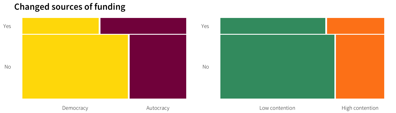
##
## ----------------------------
## Changed sources of funding
## ----------------------------
## Table counts                             Table counts
## target.regime.type Democracy Autocracy                    |  potential.contentiousness Low contention High contention
## response                                                  |  response
## No                       177        95                    |  No                                   191              81
## Yes                       32        36                    |  Yes                                   44              24
##
## Expected values                              Expected values
##         target.regime.type                        |          potential.contentiousness
## response Democracy Autocracy                      |  response Low contention High contention
##      No      167.2     104.8                      |       No             188              84
##      Yes      41.8      26.2                      |       Yes             47              21
##
## Row proporitions                         Row proporitions
## target.regime.type Democracy Autocracy                    |  potential.contentiousness Low contention High contention
## response                                                  |  response
## No                 0.6507353 0.3492647                    |  No                             0.7022059       0.2977941
## Yes                0.4705882 0.5294118                    |  Yes                            0.6470588       0.3529412
##
## Column proporitions                          Column proporitions
## target.regime.type Democracy Autocracy                    |  potential.contentiousness Low contention High contention
## response                                                  |  response
## No                 0.8468900 0.7251908                    |  No                             0.8127660       0.7714286
## Yes                0.1531100 0.2748092                    |  Yes                            0.1872340       0.2285714
##
## Chi-squared test for table                       Chi-squared test for table
##
##  Pearson's Chi-squared test with Yates' continuity correction        Pearson's Chi-squared test with Yates' continuity correction
##
## data:  ftable(cat.table)                     data:  ftable(cat.table)
## X-squared = 6.7129, df = 1, p-value = 0.009572                |  X-squared = 0.53825, df = 1, p-value = 0.4632
##
## Cramer's V                               Cramer's V
## [1] 0.1480667                                 |  [1] 0.04774553
##
## Pearson residuals                            Pearson residuals
## 2 is used as critical value by convention                2 is used as critical value by convention
## target.regime.type  Democracy  Autocracy              |  potential.contentiousness Low contention High contention
## response                                              |  response
## No                  0.7578931 -0.9572942              |  No                             0.2187975      -0.3273268
## Yes                -1.5157862  1.9145884              |  Yes                           -0.4375950       0.6546537
##
## Components of chi-squared                        Components of chi-squared
## Critical value (0.05 with 1 df) is 3.84                  Critical value (0.05 with 1 df) is 3.84
## target.regime.type Democracy Autocracy                    |  potential.contentiousness Low contention High contention
## response                                                  |  response
## No                 0.5744019 0.9164122                    |  No                            0.04787234      0.10714286
## Yes                2.2976077 3.6656489                    |  Yes                           0.19148936      0.42857143
##
## p for components                         p for components
## target.regime.type Democracy Autocracy                    |  potential.contentiousness Low contention High contention
## response                                                  |  response
## No                     0.449     0.338                    |  No                                 0.827           0.743
## Yes                    0.130     0.056                    |  Yes                                0.662           0.513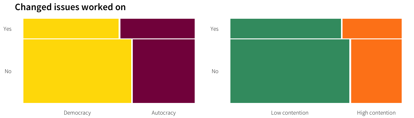
##
## --------------------------
## Changed issues worked on
## --------------------------
## Table counts                             Table counts
## target.regime.type Democracy Autocracy                    |  potential.contentiousness Low contention High contention
## response                                                  |  response
## No                       181       104                    |  No                                   200              85
## Yes                       50        39                    |  Yes                                   58              31
##
## Expected values                              Expected values
##         target.regime.type                        |          potential.contentiousness
## response Democracy Autocracy                      |  response Low contention High contention
##      No  176.02941 108.97059                      |       No       196.60428        88.39572
##      Yes  54.97059  34.02941                      |       Yes       61.39572        27.60428
##
## Row proporitions                         Row proporitions
## target.regime.type Democracy Autocracy                    |  potential.contentiousness Low contention High contention
## response                                                  |  response
## No                 0.6350877 0.3649123                    |  No                             0.7017544       0.2982456
## Yes                0.5617978 0.4382022                    |  Yes                            0.6516854       0.3483146
##
## Column proporitions                          Column proporitions
## target.regime.type Democracy Autocracy                    |  potential.contentiousness Low contention High contention
## response                                                  |  response
## No                 0.7835498 0.7272727                    |  No                             0.7751938       0.7327586
## Yes                0.2164502 0.2727273                    |  Yes                            0.2248062       0.2672414
##
## Chi-squared test for table                       Chi-squared test for table
##
##  Pearson's Chi-squared test with Yates' continuity correction        Pearson's Chi-squared test with Yates' continuity correction
##
## data:  ftable(cat.table)                     data:  ftable(cat.table)
## X-squared = 1.2478, df = 1, p-value = 0.264               |  X-squared = 0.57785, df = 1, p-value = 0.4472
##
## Cramer's V                               Cramer's V
## [1] 0.06422261                                |  [1] 0.04609432
##
## Pearson residuals                            Pearson residuals
## 2 is used as critical value by convention                2 is used as critical value by convention
## target.regime.type  Democracy  Autocracy              |  potential.contentiousness Low contention High contention
## response                                              |  response
## No                  0.3746409 -0.4761603              |  No                             0.2421785      -0.3611740
## Yes                -0.6704133  0.8520804              |  Yes                           -0.4333742       0.6463145
##
## Components of chi-squared                        Components of chi-squared
## Critical value (0.05 with 1 df) is 3.84                  Critical value (0.05 with 1 df) is 3.84
## target.regime.type Democracy Autocracy                    |  potential.contentiousness Low contention High contention
## response                                                  |  response
## No                 0.1403558 0.2267286                    |  No                            0.05865044      0.13044667
## Yes                0.4494539 0.7260410                    |  Yes                           0.18781321      0.41772248
##
## p for components                         p for components
## target.regime.type Democracy Autocracy                    |  potential.contentiousness Low contention High contention
## response                                                  |  response
## No                     0.708     0.634                    |  No                                 0.809           0.718
## Yes                    0.503     0.394                    |  Yes                                0.665           0.518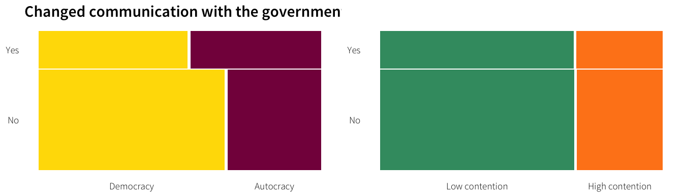
##
## -------------------------------------------
## Changed communication with the government
## -------------------------------------------
## Table counts                             Table counts
## target.regime.type Democracy Autocracy                    |  potential.contentiousness Low contention High contention
## response                                                  |  response
## No                       167        84                    |  No                                   174              77
## Yes                       50        44                    |  Yes                                   65              29
##
## Expected values                              Expected values
##         target.regime.type                        |          potential.contentiousness
## response Democracy Autocracy                      |  response Low contention High contention
##      No  157.87536  93.12464                      |       No       173.88116        77.11884
##      Yes  59.12464  34.87536                      |       Yes       65.11884        28.88116
##
## Row proporitions                         Row proporitions
## target.regime.type Democracy Autocracy                    |  potential.contentiousness Low contention High contention
## response                                                  |  response
## No                 0.6653386 0.3346614                    |  No                             0.6932271       0.3067729
## Yes                0.5319149 0.4680851                    |  Yes                            0.6914894       0.3085106
##
## Column proporitions                          Column proporitions
## target.regime.type Democracy Autocracy                    |  potential.contentiousness Low contention High contention
## response                                                  |  response
## No                 0.7695853 0.6562500                    |  No                             0.7280335       0.7264151
## Yes                0.2304147 0.3437500                    |  Yes                            0.2719665       0.2735849
##
## Chi-squared test for table                       Chi-squared test for table
##
##  Pearson's Chi-squared test with Yates' continuity correction        Pearson's Chi-squared test with Yates' continuity correction
##
## data:  ftable(cat.table)                     data:  ftable(cat.table)
## X-squared = 4.6609, df = 1, p-value = 0.03086                 |  X-squared = 1.7481e-30, df = 1, p-value = 1
##
## Cramer's V                               Cramer's V
## [1] 0.12297                               |  [1] 0.001676993
##
## Pearson residuals                            Pearson residuals
## 2 is used as critical value by convention                2 is used as critical value by convention
## target.regime.type  Democracy  Autocracy              |  potential.contentiousness Low contention High contention
## response                                              |  response
## No                  0.7262037 -0.9455475              |  No                           0.009012359    -0.013532702
## Yes                -1.1866739  1.5450988              |  Yes                         -0.014726903     0.022113498
##
## Components of chi-squared                        Components of chi-squared
## Critical value (0.05 with 1 df) is 3.84                  Critical value (0.05 with 1 df) is 3.84
## target.regime.type Democracy Autocracy                    |  potential.contentiousness Low contention High contention
## response                                                  |  response
## No                 0.5273718 0.8940600                    |  No                          8.122262e-05    1.831340e-04
## Yes                1.4081949 2.3873304                    |  Yes                         2.168817e-04    4.890068e-04
##
## p for components                         p for components
## target.regime.type Democracy Autocracy                    |  potential.contentiousness Low contention High contention
## response                                                  |  response
## No                     0.468     0.344                    |  No                                 0.993           0.989
## Yes                    0.235     0.122                    |  Yes                                0.988           0.982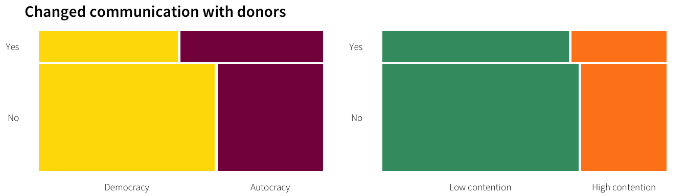
##
## -----------------------------------
## Changed communication with donors
## -----------------------------------
## Table counts                             Table counts
## target.regime.type Democracy Autocracy                    |  potential.contentiousness Low contention High contention
## response                                                  |  response
## No                       165        99                    |  No                                   184              80
## Yes                       38        39                    |  Yes                                   51              26
##
## Expected values                              Expected values
##         target.regime.type                        |          potential.contentiousness
## response Democracy Autocracy                      |  response Low contention High contention
##      No  157.16129 106.83871                      |       No       181.93548        82.06452
##      Yes  45.83871  31.16129                      |       Yes       53.06452        23.93548
##
## Row proporitions                         Row proporitions
## target.regime.type Democracy Autocracy                    |  potential.contentiousness Low contention High contention
## response                                                  |  response
## No                 0.6250000 0.3750000                    |  No                             0.6969697       0.3030303
## Yes                0.4935065 0.5064935                    |  Yes                            0.6623377       0.3376623
##
## Column proporitions                          Column proporitions
## target.regime.type Democracy Autocracy                    |  potential.contentiousness Low contention High contention
## response                                                  |  response
## No                 0.8128079 0.7173913                    |  No                             0.7829787       0.7547170
## Yes                0.1871921 0.2826087                    |  Yes                            0.2170213       0.2452830
##
## Chi-squared test for table                       Chi-squared test for table
##
##  Pearson's Chi-squared test with Yates' continuity correction        Pearson's Chi-squared test with Yates' continuity correction
##
## data:  ftable(cat.table)                     data:  ftable(cat.table)
## X-squared = 3.75, df = 1, p-value = 0.05281               |  X-squared = 0.19167, df = 1, p-value = 0.6615
##
## Cramer's V                               Cramer's V
## [1] 0.1120119                                 |  [1] 0.03128517
##
## Pearson residuals                            Pearson residuals
## 2 is used as critical value by convention                2 is used as critical value by convention
## target.regime.type  Democracy  Autocracy              |  potential.contentiousness Low contention High contention
## response                                              |  response
## No                  0.6252760 -0.7583685              |  No                             0.1530592      -0.2278980
## Yes                -1.1577863  1.4042255              |  Yes                           -0.2834107       0.4219852
##
## Components of chi-squared                        Components of chi-squared
## Critical value (0.05 with 1 df) is 3.84                  Critical value (0.05 with 1 df) is 3.84
## target.regime.type Democracy Autocracy                    |  potential.contentiousness Low contention High contention
## response                                                  |  response
## No                 0.3909701 0.5751227                    |  No                            0.02342713      0.05193751
## Yes                1.3404690 1.9718493                    |  Yes                           0.08032160      0.17807147
##
## p for components                         p for components
## target.regime.type Democracy Autocracy                    |  potential.contentiousness Low contention High contention
## response                                                  |  response
## No                     0.532     0.448                    |  No                                 0.878           0.820
## Yes                    0.247     0.160                    |  Yes                                0.777           0.673
##
## -----------------------------
## Changed locations worked in
## -----------------------------
## Table counts                             Table counts
## target.regime.type Democracy Autocracy                    |  potential.contentiousness Low contention High contention
## response                                                  |  response
## No                       178        87                    |  No                                   185              80
## Yes                       42        44                    |  Yes                                   58              28
##
## Expected values                              Expected values
##         target.regime.type                        |          potential.contentiousness
## response Democracy Autocracy                      |  response Low contention High contention
##      No  166.09687  98.90313                      |       No       183.46154        81.53846
##      Yes  53.90313  32.09687                      |       Yes       59.53846        26.46154
##
## Row proporitions                         Row proporitions
## target.regime.type Democracy Autocracy                    |  potential.contentiousness Low contention High contention
## response                                                  |  response
## No                 0.6716981 0.3283019                    |  No                             0.6981132       0.3018868
## Yes                0.4883721 0.5116279                    |  Yes                            0.6744186       0.3255814
##
## Column proporitions                          Column proporitions
## target.regime.type Democracy Autocracy                    |  potential.contentiousness Low contention High contention
## response                                                  |  response
## No                 0.8090909 0.6641221                    |  No                             0.7613169       0.7407407
## Yes                0.1909091 0.3358779                    |  Yes                            0.2386831       0.2592593
##
## Chi-squared test for table                       Chi-squared test for table
##
##  Pearson's Chi-squared test with Yates' continuity correction        Pearson's Chi-squared test with Yates' continuity correction
##
## data:  ftable(cat.table)                     data:  ftable(cat.table)
## X-squared = 8.5611, df = 1, p-value = 0.003434                |  X-squared = 0.07797, df = 1, p-value = 0.7801
##
## Cramer's V                               Cramer's V
## [1] 0.1630232                                 |  [1] 0.02208038
##
## Pearson residuals                            Pearson residuals
## 2 is used as critical value by convention                2 is used as critical value by convention
## target.regime.type  Democracy  Autocracy              |  potential.contentiousness Low contention High contention
## response                                              |  response
## No                  0.9235929 -1.1968957              |  No                             0.1135832      -0.1703748
## Yes                -1.6212661  2.1010191              |  Yes                           -0.1993829       0.2990743
##
## Components of chi-squared                        Components of chi-squared
## Critical value (0.05 with 1 df) is 3.84                  Critical value (0.05 with 1 df) is 3.84
## target.regime.type Democracy Autocracy                    |  potential.contentiousness Low contention High contention
## response                                                  |  response
## No                 0.8530239 1.4325592                    |  No                            0.01290114      0.02902758
## Yes                2.6285039 4.4142813                    |  Yes                           0.03975353      0.08944544
##
## p for components                         p for components
## target.regime.type Democracy Autocracy                    |  potential.contentiousness Low contention High contention
## response                                                  |  response
## No                     0.356     0.231                    |  No                                 0.910           0.865
## Yes                    0.105     0.036                    |  Yes                                0.842           0.765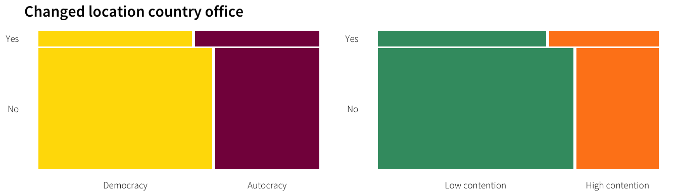
##
## ---------------------------------
## Changed location country office
## ---------------------------------
## Table counts                             Table counts
## target.regime.type Democracy Autocracy                    |  potential.contentiousness Low contention High contention
## response                                                  |  response
## No                       183       110                    |  No                                   206              87
## Yes                       21        17                    |  Yes                                   23              15
##
## Expected values                              Expected values
##         target.regime.type                        |          potential.contentiousness
## response Democracy Autocracy                      |  response Low contention High contention
##      No  180.58006 112.41994                      |       No       202.70997        90.29003
##      Yes  23.41994  14.58006                      |       Yes       26.29003        11.70997
##
## Row proporitions                         Row proporitions
## target.regime.type Democracy Autocracy                    |  potential.contentiousness Low contention High contention
## response                                                  |  response
## No                 0.6245734 0.3754266                    |  No                             0.7030717       0.2969283
## Yes                0.5526316 0.4473684                    |  Yes                            0.6052632       0.3947368
##
## Column proporitions                          Column proporitions
## target.regime.type Democracy Autocracy                    |  potential.contentiousness Low contention High contention
## response                                                  |  response
## No                 0.8970588 0.8661417                    |  No                             0.8995633       0.8529412
## Yes                0.1029412 0.1338583                    |  Yes                            0.1004367       0.1470588
##
## Chi-squared test for table                       Chi-squared test for table
##
##  Pearson's Chi-squared test with Yates' continuity correction        Pearson's Chi-squared test with Yates' continuity correction
##
## data:  ftable(cat.table)                     data:  ftable(cat.table)
## X-squared = 0.46342, df = 1, p-value = 0.496              |  X-squared = 1.0855, df = 1, p-value = 0.2975
##
## Cramer's V                               Cramer's V
## [1] 0.04716176                                |  [1] 0.06752809
##
## Pearson residuals                            Pearson residuals
## 2 is used as critical value by convention                2 is used as critical value by convention
## target.regime.type  Democracy  Autocracy              |  potential.contentiousness Low contention High contention
## response                                              |  response
## No                  0.1800817 -0.2282353              |  No                             0.2310800      -0.3462422
## Yes                -0.5000479  0.6337601              |  Yes                           -0.6416591       0.9614396
##
## Components of chi-squared                        Components of chi-squared
## Critical value (0.05 with 1 df) is 3.84                  Critical value (0.05 with 1 df) is 3.84
## target.regime.type  Democracy  Autocracy              |  potential.contentiousness Low contention High contention
## response                                              |  response
## No                 0.03242943 0.05209136              |  No                            0.05339796      0.11988365
## Yes                0.25004794 0.40165180              |  Yes                           0.41172637      0.92436607
##
## p for components                         p for components
## target.regime.type Democracy Autocracy                    |  potential.contentiousness Low contention High contention
## response                                                  |  response
## No                     0.857     0.819                    |  No                                 0.817           0.729
## Yes                    0.617     0.526                    |  Yes                                0.521           0.336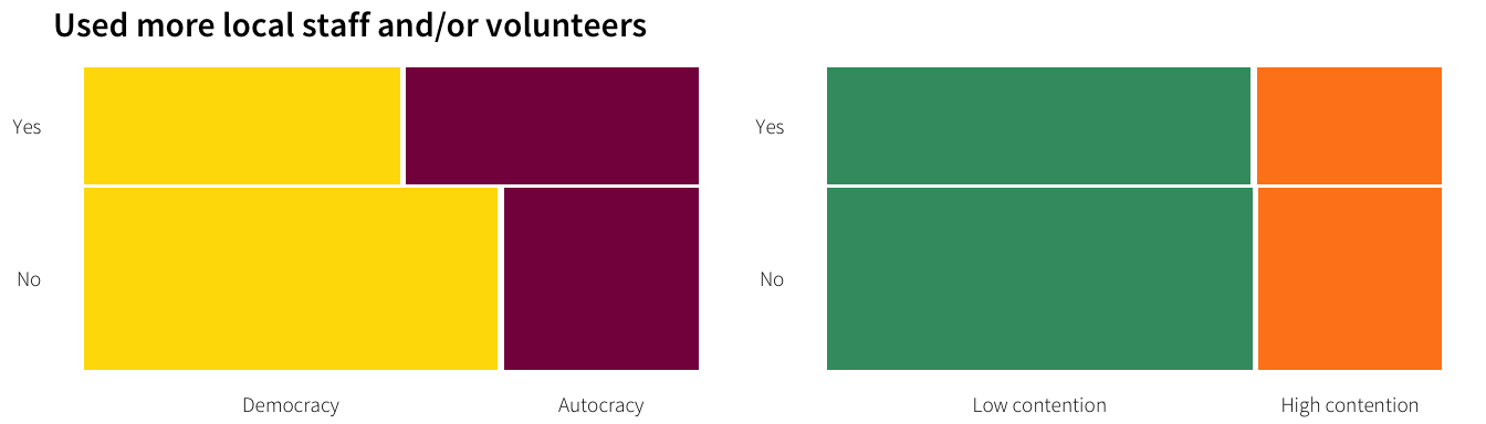
##
## -----------------------------------------
## Used more local staff and/or volunteers
## -----------------------------------------
## Table counts                             Table counts
## target.regime.type Democracy Autocracy                    |  potential.contentiousness Low contention High contention
## response                                                  |  response
## No                       142        67                    |  No                                   146              63
## Yes                       70        65                    |  Yes                                   94              41
##
## Expected values                              Expected values
##         target.regime.type                        |          potential.contentiousness
## response Democracy Autocracy                      |  response Low contention High contention
##      No  128.80233  80.19767                      |       No       145.81395        63.18605
##      Yes  83.19767  51.80233                      |       Yes       94.18605        40.81395
##
## Row proporitions                         Row proporitions
## target.regime.type Democracy Autocracy                    |  potential.contentiousness Low contention High contention
## response                                                  |  response
## No                 0.6794258 0.3205742                    |  No                             0.6985646       0.3014354
## Yes                0.5185185 0.4814815                    |  Yes                            0.6962963       0.3037037
##
## Column proporitions                          Column proporitions
## target.regime.type Democracy Autocracy                    |  potential.contentiousness Low contention High contention
## response                                                  |  response
## No                 0.6698113 0.5075758                    |  No                             0.6083333       0.6057692
## Yes                0.3301887 0.4924242                    |  Yes                            0.3916667       0.3942308
##
## Chi-squared test for table                       Chi-squared test for table
##
##  Pearson's Chi-squared test with Yates' continuity correction        Pearson's Chi-squared test with Yates' continuity correction
##
## data:  ftable(cat.table)                     data:  ftable(cat.table)
## X-squared = 8.3125, df = 1, p-value = 0.003937                |  X-squared = 1.0288e-29, df = 1, p-value = 1
##
## Cramer's V                               Cramer's V
## [1] 0.1615701                                 |  [1] 0.002411669
##
## Pearson residuals                            Pearson residuals
## 2 is used as critical value by convention                2 is used as critical value by convention
## target.regime.type Democracy Autocracy                    |  potential.contentiousness Low contention High contention
## response                                                  |  response
## No                  1.162882 -1.473725                    |  No                            0.01540714     -0.02340512
## Yes                -1.446911  1.833677                    |  Yes                          -0.01917027      0.02912173
##
## Components of chi-squared                        Components of chi-squared
## Critical value (0.05 with 1 df) is 3.84                  Critical value (0.05 with 1 df) is 3.84
## target.regime.type Democracy Autocracy                    |  potential.contentiousness Low contention High contention
## response                                                  |  response
## No                  1.352294  2.171866                    |  No                          0.0002373799    0.0005477998
## Yes                 2.093551  3.362370                    |  Yes                         0.0003674993    0.0008480753
##
## p for components                         p for components
## target.regime.type Democracy Autocracy                    |  potential.contentiousness Low contention High contention
## response                                                  |  response
## No                     0.245     0.141                    |  No                                 0.988           0.981
## Yes                    0.148     0.067                    |  Yes                                0.985           0.977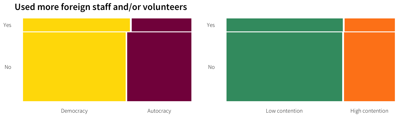
##
## -------------------------------------------
## Used more foreign staff and/or volunteers
## -------------------------------------------
## Table counts                             Table counts
## target.regime.type Democracy Autocracy                    |  potential.contentiousness Low contention High contention
## response                                                  |  response
## No                       171       107                    |  No                                   193              85
## Yes                       34        19                    |  Yes                                   37              16
##
## Expected values                              Expected values
##         target.regime.type                        |          potential.contentiousness
## response Democracy Autocracy                      |  response Low contention High contention
##      No  172.17523 105.82477                      |       No       193.17221        84.82779
##      Yes  32.82477  20.17523                      |       Yes       36.82779        16.17221
##
## Row proporitions                         Row proporitions
## target.regime.type Democracy Autocracy                    |  potential.contentiousness Low contention High contention
## response                                                  |  response
## No                 0.6151079 0.3848921                    |  No                             0.6942446       0.3057554
## Yes                0.6415094 0.3584906                    |  Yes                            0.6981132       0.3018868
##
## Column proporitions                          Column proporitions
## target.regime.type Democracy Autocracy                    |  potential.contentiousness Low contention High contention
## response                                                  |  response
## No                 0.8341463 0.8492063                    |  No                             0.8391304       0.8415842
## Yes                0.1658537 0.1507937                    |  Yes                            0.1608696       0.1584158
##
## Chi-squared test for table                       Chi-squared test for table
##
##  Pearson's Chi-squared test with Yates' continuity correction        Pearson's Chi-squared test with Yates' continuity correction
##
## data:  ftable(cat.table)                     data:  ftable(cat.table)
## X-squared = 0.043445, df = 1, p-value = 0.8349                |  X-squared = 1.637e-30, df = 1, p-value = 1
##
## Cramer's V                               Cramer's V
## [1] 0.01994009                                |  [1] 0.003080987
##
## Pearson residuals                            Pearson residuals
## 2 is used as critical value by convention                2 is used as critical value by convention
## target.regime.type   Democracy   Autocracy                |  potential.contentiousness Low contention High contention
## response                                                  |  response
## No                 -0.08956458  0.11424256                |  No                           -0.01239009      0.01869725
## Yes                 0.20512601 -0.26164497                |  Yes                           0.02837651     -0.04282154
##
## Components of chi-squared                        Components of chi-squared
## Critical value (0.05 with 1 df) is 3.84                  Critical value (0.05 with 1 df) is 3.84
## target.regime.type   Democracy   Autocracy                |  potential.contentiousness Low contention High contention
## response                                                  |  response
## No                 0.008021813 0.013051363                |  No                          0.0001535144    0.0003495872
## Yes                0.042076681 0.068458093                |  Yes                         0.0008052264    0.0018336839
##
## p for components                         p for components
## target.regime.type Democracy Autocracy                    |  potential.contentiousness Low contention High contention
## response                                                  |  response
## No                     0.929     0.909                    |  No                                 0.990           0.985
## Yes                    0.837     0.794                    |  Yes                                0.977           0.966
Discussions with government
Regime type
INGOs working in autocracies are far more likely to have discussed NGO regulations with their host governments—the majority actually have (54% of those responding “yes” work in autocracies; 32% of those working in autocracies responded “yes”), and the difference is statistically significant. This is likely because INGOs working in autocracies have more of a reason to discuss the regulations, as they see more regulations in general.
df.discuss.regime <- survey.countries.clean %>%
  filter(!is.na(Q4.22)) %>%
  filter(Q4.22 != "Don't know") %>%
  mutate(Q4.22 = droplevels(Q4.22),
         Q4.22 = factor(Q4.22, levels=rev(levels(Q4.22)))) %>%
  select(Q4.22, target.regime.type)

plot.discuss.regime <- prodplot(df.discuss.regime,
                                    ~ target.regime.type + Q4.22, mosaic("h"),
                                    colour=NA) +
  aes(fill=target.regime.type, colour="white") +
  scale_fill_manual(values=ath.palette("regime"), name=NULL) +
  guides(fill=FALSE) +
  labs(title="Discussions about regulations, by regime type",
       subtitle="Q4.22: Has your organization discussed NGO regulations with government officials in `target_country`?") +
  theme_ath() + theme(axis.title=element_blank(),
                      panel.grid=element_blank())
plot.discuss.regime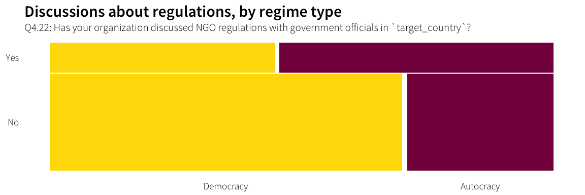
discuss.table <- df.discuss.regime %>%
  xtabs(~ Q4.22 + target.regime.type, .)

analyze.cat.var(discuss.table)
## Table counts
## target.regime.type Democracy Autocracy
## Q4.22
## No 257 107
## Yes 50 61
##
## Expected values
## target.regime.type
## Q4.22 Democracy Autocracy
## No 235.25895 128.74105
## Yes 71.74105 39.25895
##
## Row proporitions
## target.regime.type Democracy Autocracy
## Q4.22
## No 0.7060440 0.2939560
## Yes 0.4504505 0.5495495
##
## Column proporitions
## target.regime.type Democracy Autocracy
## Q4.22
## No 0.8371336 0.6369048
## Yes 0.1628664 0.3630952
##
## Chi-squared test for table
##
## Pearson's Chi-squared test with Yates' continuity correction
##
## data: ftable(cat.table)
## X-squared = 23.204, df = 1, p-value = 1.457e-06
##
## Cramer's V
## [1] 0.2262237
##
## Pearson residuals
## 2 is used as critical value by convention
## target.regime.type Democracy Autocracy
## Q4.22
## No 1.417449 -1.916117
## Yes -2.566828 3.469854
##
## Components of chi-squared
## Critical value (0.05 with 1 df) is 3.84
## target.regime.type Democracy Autocracy
## Q4.22
## No 2.009162 3.671505
## Yes 6.588604 12.039889
##
## p for components
## target.regime.type Democracy Autocracy
## Q4.22
## No 0.156 0.055
## Yes 0.010 0.001Potential contentiousness
There’s no difference across issue areas in whether or not an INGO discusses regulations with the government—the same proportion (66% haven’t discussed; 20% have; 10% don’t know) holds across both levels of potential contentiousness.
df.discuss.issue <- survey.countries.clean %>%
  filter(!is.na(Q4.22)) %>%
  filter(Q4.22 != "Don't know") %>%
  mutate(Q4.22 = droplevels(Q4.22),
         Q4.22 = factor(Q4.22, levels=rev(levels(Q4.22)))) %>%
  select(Q4.22, potential.contentiousness)

plot.discuss.issue <- prodplot(df.discuss.issue,
                               ~ potential.contentiousness + Q4.22, mosaic("h"),
                               colour=NA) +
  aes(fill=potential.contentiousness, colour="white") +
  scale_fill_manual(values=ath.palette("contention"), name=NULL) +
  guides(fill=FALSE) +
  labs(title="Discussions about regulations, by issue",
       subtitle="Q4.22: Has your organization discussed NGO regulations with government officials in `target_country`?") +
  theme_ath() + theme(axis.title=element_blank(),
                      panel.grid=element_blank())
plot.discuss.issue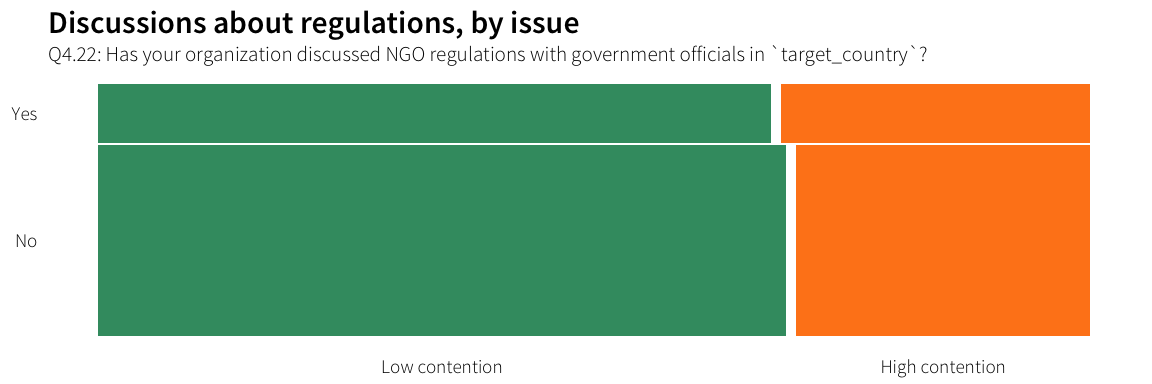
discuss.issue.table <- df.discuss.issue %>%
  xtabs(~ Q4.22 + potential.contentiousness, .)

analyze.cat.var(discuss.issue.table)
## Table counts
## potential.contentiousness Low contention High contention
## Q4.22
## No 255 109
## Yes 76 35
##
## Expected values
## potential.contentiousness
## Q4.22 Low contention High contention
## No 253.65053 110.34947
## Yes 77.34947 33.65053
##
## Row proporitions
## potential.contentiousness Low contention High contention
## Q4.22
## No 0.7005495 0.2994505
## Yes 0.6846847 0.3153153
##
## Column proporitions
## potential.contentiousness Low contention High contention
## Q4.22
## No 0.7703927 0.7569444
## Yes 0.2296073 0.2430556
##
## Chi-squared test for table
##
## Pearson's Chi-squared test with Yates' continuity correction
##
## data: ftable(cat.table)
## X-squared = 0.040157, df = 1, p-value = 0.8412
##
## Cramer's V
## [1] 0.01460665
##
## Pearson residuals
## 2 is used as critical value by convention
## potential.contentiousness Low contention High contention
## Q4.22
## No 0.08473182 -0.12846336
## Yes -0.15343899 0.23263148
##
## Components of chi-squared
## Critical value (0.05 with 1 df) is 3.84
## potential.contentiousness Low contention High contention
## Q4.22
## No 0.007179481 0.016502836
## Yes 0.023543524 0.054117407
##
## p for components
## potential.contentiousness Low contention High contention
## Q4.22
## No 0.932 0.898
## Yes 0.878 0.816Attempts to change regulations
Regime type
Most INGOs don’t attempt to change regulations, but those that do are most likely to work in autocracies (and the difference is significant). Additionally, only 8% of INGOs working in democracies have attempted to change regulations, while 16% of those working in autocracies have, despite the fact that the legislative process is much more difficult to navigate in autocracies. INGOs appear to be more likely to engage in the political process to adjust regulations despite these challenges.
df.change.regs.regime <- survey.countries.clean %>%
  filter(!is.na(Q4.23)) %>%
  filter(Q4.23 != "Don't know") %>%
  mutate(Q4.23 = droplevels(Q4.23),
         Q4.23 = factor(Q4.23, levels=rev(levels(Q4.23)))) %>%
  select(Q4.23, target.regime.type)

plot.change.regs.regime <- prodplot(df.change.regs.regime,
                                ~ target.regime.type + Q4.23, mosaic("h"),
                                colour=NA) +
  aes(fill=target.regime.type, colour="white") +
  scale_fill_manual(values=ath.palette("regime"), name=NULL) +
  guides(fill=FALSE) +
  labs(title="Attempts to change regulations, by regime type",
       subtitle="Q4.23: Has your organization tried to change NGO regulations in `target_country`?") +
  theme_ath() + theme(axis.title=element_blank(),
                      panel.grid=element_blank())
plot.change.regs.regime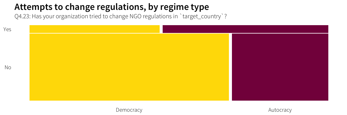
change.regs.table <- df.change.regs.regime %>%
  xtabs(~ Q4.23 + target.regime.type, .)

analyze.cat.var(change.regs.table)
## Table counts
## target.regime.type Democracy Autocracy
## Q4.23
## No 295 143
## Yes 22 28
##
## Expected values
## target.regime.type
## Q4.23 Democracy Autocracy
## No 284.52049 153.47951
## Yes 32.47951 17.52049
##
## Row proporitions
## target.regime.type Democracy Autocracy
## Q4.23
## No 0.673516 0.326484
## Yes 0.440000 0.560000
##
## Column proporitions
## target.regime.type Democracy Autocracy
## Q4.23
## No 0.93059937 0.83625731
## Yes 0.06940063 0.16374269
##
## Chi-squared test for table
##
## Pearson's Chi-squared test with Yates' continuity correction
##
## data: ftable(cat.table)
## X-squared = 9.7494, df = 1, p-value = 0.001794
##
## Cramer's V
## [1] 0.1484263
##
## Pearson residuals
## 2 is used as critical value by convention
## target.regime.type Democracy Autocracy
## Q4.23
## No 0.6212754 -0.8458935
## Yes -1.8388071 2.5036162
##
## Components of chi-squared
## Critical value (0.05 with 1 df) is 3.84
## target.regime.type Democracy Autocracy
## Q4.23
## No 0.3859831 0.7155359
## Yes 3.3812117 6.2680941
##
## p for components
## target.regime.type Democracy Autocracy
## Q4.23
## No 0.534 0.398
## Yes 0.066 0.012Potential contentiousness
There’s also a difference across issue area. INGOs working on highly contentious issues are more likely to try to change regulations, similar to regime type. The difference is statistically significant overall, but is not driven by a single significant cell (though yes + high comes close).
df.change.regs.issue <- survey.countries.clean %>%
  filter(!is.na(Q4.23)) %>%
  filter(Q4.23 != "Don't know") %>%
  mutate(Q4.23 = droplevels(Q4.23),
         Q4.23 = factor(Q4.23, levels=rev(levels(Q4.23)))) %>%
  select(Q4.23, potential.contentiousness)

plot.change.regs.issue <- prodplot(df.change.regs.issue,
                               ~ potential.contentiousness + Q4.23, mosaic("h"),
                               colour=NA) +
  aes(fill=potential.contentiousness, colour="white") +
  scale_fill_manual(values=ath.palette("contention"), name=NULL) +
  guides(fill=FALSE) +
  labs(title="Attempts to change regulations, by issue",
       subtitle="Q4.23: Has your organization tried to change NGO regulations in `target_country`?") +
  theme_ath() + theme(axis.title=element_blank(),
                      panel.grid=element_blank())
plot.change.regs.issue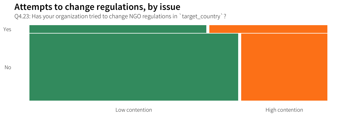
change.regs.issue.table <- df.change.regs.issue %>%
  xtabs(~ Q4.23 + potential.contentiousness, .)

analyze.cat.var(change.regs.issue.table)
## Table counts
## potential.contentiousness Low contention High contention
## Q4.23
## No 310 128
## Yes 30 20
##
## Expected values
## potential.contentiousness
## Q4.23 Low contention High contention
## No 305.16393 132.83607
## Yes 34.83607 15.16393
##
## Row proporitions
## potential.contentiousness Low contention High contention
## Q4.23
## No 0.7077626 0.2922374
## Yes 0.6000000 0.4000000
##
## Column proporitions
## potential.contentiousness Low contention High contention
## Q4.23
## No 0.91176471 0.86486486
## Yes 0.08823529 0.13513514
##
## Chi-squared test for table
##
## Pearson's Chi-squared test with Yates' continuity correction
##
## data: ftable(cat.table)
## X-squared = 1.9827, df = 1, p-value = 0.1591
##
## Cramer's V
## [1] 0.07109182
##
## Pearson residuals
## 2 is used as critical value by convention
## potential.contentiousness Low contention High contention
## Q4.23
## No 0.2768379 -0.4195987
## Yes -0.8193654 1.2418989
##
## Components of chi-squared
## Critical value (0.05 with 1 df) is 3.84
## potential.contentiousness Low contention High contention
## Q4.23
## No 0.07663923 0.17606311
## Yes 0.67135969 1.54231280
##
## p for components
## potential.contentiousness Low contention High contention
## Q4.23
## No 0.782 0.675
## Yes 0.413 0.214Testing hypotheses
My claim:
If an INGO does not make one of these three adjustments—shifting its ideal point, increasing its operational flexibility, or becoming essential for the regime—it runs a high risk of expulsion.
What influences feelings of restriction? Main hypotheses:
- Normative principles and ideals
- Issue area
- Instrumental flexibility
- Size
- Type of funding
- Collaboration
- Alignment with regime preferences